Biological Rotation Age of Community Teak (Tectona grandis) Plantation Based on the Volume, Biomass, and Price Growth Curve Determined through the Analysis of Its Tree Ring Digitization

Abstract

Teak (Tectona grandis) is a deciduous tree producing a popular, expensive, fancy timber with versatile utilization. The teak population and its habitats in the natural forest have been decreasing consistently; thus, the IUCN Red List classifies it as an endangered species. Teak tree logging from its native natural forest is banned, and commercial teak timber can only be harvested from the plantation. People plant teak on their private lands or in the community forest to meet the increasing demand. This study analyzed the annual tree rings of a teak disk taken from the community plantation and aimed to determine its biological rotation age. Tree ring interpretation provides the increment and growth that are mandatory fundamental components of knowledge in sustainable forest management. It may also decipher the tree’s biography, which contains information about past climate and future predictions responding to climate change. All of the disk’s annual tree rings were digitized, transformed, and then curve-fitted using an elliptical polar form of non-linear regression. The best-fitted curve estimation of every annual tree ring was employed to determine their age-related diameter and basal area, and then allometric equations estimated the above-ground biomass and clear-bole volume. The continuous and discrete formula fit the growth curve well, and this study determined that Chapman-Richards is the best fit among others. The growth curve, current annual increment (CAI), and mean annual increment (MAI) were graphed based on the clear-bole volume, above-ground biomass, and log timber price. The CAI and MAI intersections result in 28, 30, and 86 years of optimum harvesting periods when the growth calculation is based on volume, above-ground biomass, and log timber price, respectively. These results identified that the teak plantation is a sustainable and highly valuable asset to inherit with long-term positive benefits. The sociocultural provision of teak plants as an inheritance gift for the next generation has proven to be economically and ecologically beneficial.

1. Introduction

Teak or Indian oak (Tectona grandis Linn f.), for which the local Indonesian name is jati, is a native tree species of India, Lao People’s Democratic Republic (PDR), Burma (Myanmar), and Thailand. Teak is a deciduous large tree belonging to the Lamiaceae family that naturally grows in mixed-hardwood forests. Its habitat is a terrestrial system of forest at 0–500 masl (meters above sea level) elevation. The global assessment by the IUCN Red List of Threatened Species confirms this species’ declining natural population and habitat area [1]. The area of teak-containing natural forests remains approximately only 27.9 million ha around the globe, and the remaining population is fragmented and scattered. Because it has severely declined in the last three generations and seems that it will continue to do so in the future, teak has been recently categorized as endangered [1], and harvesting it from natural forests is banned.

Teak was a symbol of royal glory for the ancient Javanese monarchy [2,3], planted in Java island more than 800 years ago by the indigenous people as a raw material with which to build palaces, fortresses, ships, and houses. The teak forests in Java were snatched, exploited, and monopolized by the United East India Company (Vereenigde Oost Indische Compagnie, VOC) and the Dutch colonial government [4,5] in the 17th–19th centuries; they were severely felled for land clearing during the Japanese occupation (1942–1945) and more recently managed by Perum Perhutani (Indonesian state-owned enterprise) after independence. Even though monoculture teak-plantation forest management has a long history, it is still incapable of fulfilling the always-increasing demand because of the stem volume’s slow growth characteristics. People plant teak on their private lands and in community forests to fill the supply–demand gap. Therefore, it is necessary to disseminate the comprehension of sustainability [6,7] to the people and community to improve the effectiveness and efficiency of natural resource management.

The stems provide the tree’s history during its lifetime, including its genetics and responses to environmental conditions. The cell dimension and density variation of earlywood and latewood formations produce gradual color sharpness and contrast that showcase tree rings on the stem’s cross-sectional area. The wood density in each tree ring also varies and can be categorized into four types (i.e., uniform, growing, unstable, and false) [8]. The diversity of a stem’s tree rings exhibits many internal and external factors related to the tree’s biography. Cambium activities, i.e., cambial cell division and xylem differentiation rate, are sensitive to water availability and significantly influenced by average rainfall magnitude [9,10]. The distance deviations between two consecutive tree rings are associated with the environmental effects on xylem production; for example, a long rainy season and higher rainfall in a year may produce more xylem, resulting in a long distance between two tree rings. In contrast, plant dehydration stress and a leafless-crown in a long drought season may yield only a thin xylem layer. The uneccentric self-weight loads, resulting from a nonsymmetric crown and leaning stem, and its combination with a flexural moment of wind load may trigger buckling [11,12] and bending [13,14,15] that produce the varied magnitudes of tensile stress in one part of the cross-sectional area and compressive stress in the other portion [16,17]. These different stress types may stir reaction wood formation. The thicker xylem layer of reaction wood formation transforms the tree ring’s shape and translocates the corresponding tree ring’s center. The tree ring’s centers and the pith may not coincide, and pith eccentricity measures this deviation [18]. The cambium differentiation forms a new layer of xylem in the outermost wood of the stem; thus, the tree ring number may represent a tree’s age. This study’s chosen species, teak (Tectona grandis), has only one period of xylem production per year, referenced in Venugopal and Krishnamurthy’s reports [19]. Every tree ring forms a closed curve that does not intersect others; the diameter of the next year’s tree ring is usually larger than the previous ones. A circle or an ellipse may fit the shape of each annual tree ring curve so that its idealized 2D plane geometric parameters [20], such as diameter, eccentricity, and basal area, can be analyzed, and then the biomass and volume can be estimated. An allometric equation, proposed by Purwanto and Silaban [21], can be employed to assess the community plantation teak’s biomass using the diameter as the indicating predictor.

The ages of a tree, represented by its tree ring count number, were plotted together with its corresponding dimensions (diameter, basal area, biomass, or volume) in a Cartesian (rectangular) diagram system to graph the growth curve. The growth curve is the mandatory available fundamental information needed to choose the silvicultural actions in a sustainable forest management system. There are four growth curve stages: exponential, linear, logarithmic, and asymptotic, which are related to the juvenile, mature, senescent, and old phases, respectively. A tree grows with an acceleration rate during the juvenile stage and constant velocity during the full vigor of maturity, decelerating during the senescent stage and an almost zero rate (stationary) during the old phase. The tree dimension (N) is the function of time (t). Such continuous logistic formulas (Verhulst-Pearl [22,23,24,25], Gompertz [26,27,28,29,30,31], von Bertalanffy [32,33,34], and Chapman–Richards [35,36]) may fit the raw observed data for generating the best-fit growth curve. The exponential modification discrete methods proposed by Bahtiar and Darwis [37,38] may also become the alternative. The best-fitted model was indicated by its high goodness of fit, represented by a high coefficient of determination (R²) and small mean square error (MSE) values.

Biological rotation age, generally determined by the intersection point of the current annual increment (CAI) and mean annual increment (MAI), is important information in the determination of a tree’s optimal cutting age for implementing a sustainable forest management system. CAI is the first derivation of the growth formula (dN/dt), where time (t) is the unit of years, while MAI is the current dimension (N_i) divided by age (t_i). Biological rotation age is commonly derived based on volume. However, in addition to being volume-based, this study proposes above-ground biomass- and price-based rotation age to determine the combination of ecological and economical optimum cutting period for a community teak plantation. A larger-diameter log is always more expensive than a smaller one. Therefore, it is necessary to consider this universal habitude to obtain the optimum economic value. This study aims to develop a method to determine the biological rotation age of a community’s teak plantation based on the volume, biomass, and price growth by analyzing its annual tree ring digitization.

2. Materials and Methods

The teak disk, taken from our laboratory collections, was analyzed. The disk was cut at the 220 cm height of an approximately 30-year-old teak that was felled in the community plantation in Central Java, Indonesia, three years ago. The 220 cm height position was chosen intentionally to avoid the tree butt swell and to keep the bottom log piece that can still be commercially sold by its owner. As an evolutionary response, a teak tree has buttresses to support its stem against internal self-weight and external loading. The specimen was air-dried in its storage cabinet. The equilibrium moisture content was approximately 15%. The disk was finely sanded using P80, P100, and P180 sandpaper consecutively to see its annual tree ring clearly, and then the cross-section was optically scanned. The picture was scaled to its original dimension (1:1).

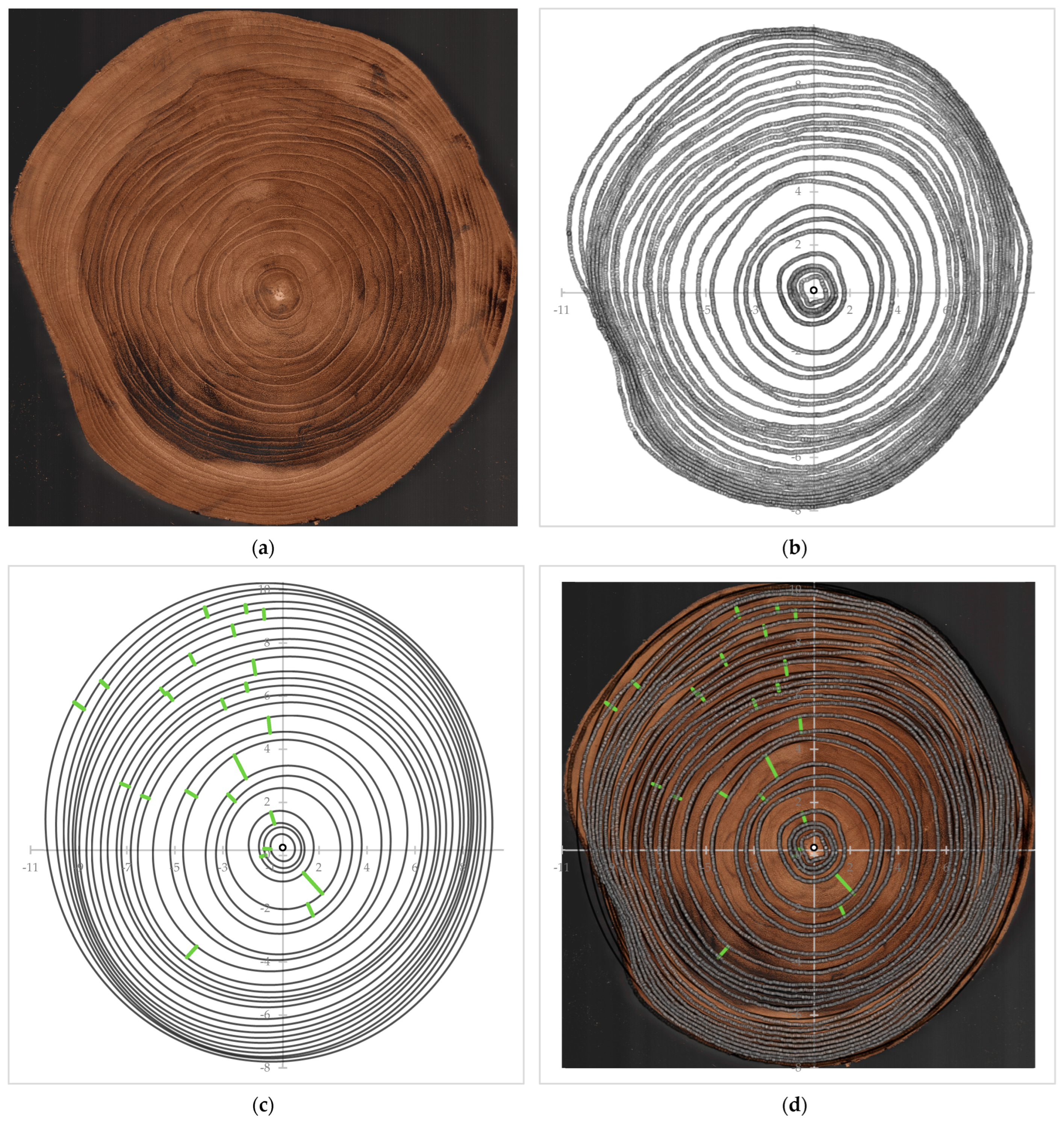
2.1. Tree Ring Circumference Digitization

The Webplot Digitizer application software version 4.6 (https://automeris.io/WebPlotDigitizer/ accessed on 1 August 2023) digitized each annual tree ring, generating data sets plotted in a Cartesian coordinate system (x, y), where the pith was located in origin (0, 0). The teak tree-ring visibility is very clear in the sapwood and heartwood portions; therefore, the anatomical features related to the growth bands’ boundary [39] were not evaluated to determine the tree ring’s entity in this study.

2.2. Annual Tree Ring Elliptical Curve Fitting

Since the data set forms a closed curve, their plots in the Cartesian coordinate system do not fulfill the prerequisite requirement of a function. One element of x (abscissa) may correspond to more than one element of y (ordinate); therefore, non-linear regression cannot directly be employed to fit it. A data transformation into a polar coordinate system (r, θ) following Equations (1)–(3) [20] is a necessary initial step to conduct the non-linear estimation of this kind of data set. The origin (0, 0) shall also be inside the closed curve to settle that every predictor value should correspond to only one response value. The non-linear regression following Equation (4), where we prefer the positive (+) sign over the negative (−) one, was employed to fit the digitization data of the tree rings that resemble rotated ellipse shapes at any arbitrary location.

$$r=\sqrt{x^2+y^2}$$

(1)

$$\theta =\mathrm{asin}\left(\frac{y}{r}\right)$$

(2)

$$\theta =\left\{\begin{array}{l}\begin{array}{l}\mathrm{asin}\left(\frac{y}{r}\right) ;\mathrm{for} 0\le \theta \le \frac{\pi }{2}\\ \pi -\mathrm{asin}\left(\frac{y}{r}\right) ;\mathrm{for} \frac{\pi }{2}\le \theta \le \pi \end{array}\\ \begin{array}{l}\pi -\mathrm{asin}\left(\frac{y}{r}\right) ;\mathrm{for} \pi \le \theta \le \frac{3\pi }{2}\\ 2\pi +\mathrm{asin}\left(\frac{y}{r}\right) ;\mathrm{for} \frac{3\pi }{2}\le \theta \le 2\pi \end{array}\end{array}\right.$$

(3)

$$r_i=\frac{r_o\left(\left(a^2-b^2\right)\sin \left({\theta }_i-k\pi \right)\sin \left({\theta }_o-k\pi \right)+b^2\cos \left({\theta }_i-{\theta }_o\right)\right)ab\sqrt{\left(a^2-b^2\right){\sin }^2\left({\theta }_i-k\pi \right)+b^2-{r_o}^2{\sin }^2\left({\theta }_i-{\theta }_o\right)}}{\left(a^2-b^2\right){\sin }^2\left({\theta }_i-k\pi \right)+b^2}+{\epsilon }_i$$

(4)

The first tree ring (the innermost one) was earliest analyzed to determine the pith’s center (r_p, θ_p), then retransformed into Cartesian to become (r_p cos θ_p, r_p sin θ_p). All digitized data points were translated from (x_i, y_i) to become (x_i − r_p cos θ_p, y_i − r_p sin θ_p), and then the adjusted (translated) Cartesian coordinates were transformed into polar (r, θ) following Equations (1)–(3). Non-linear regression was applied to fit the transformed adjusted data plot according to Equation (4) model using the Statistica 12.0 application and to estimate the parameters (a, b, r_o, θ_o, and k). The estimated parameters represent the semi-major and semi-minor (a, b) axes, the center location of the ellipse (r_o, θ_o), and the rotation angle (kπ) about the center. The Desmos graphing calculator guessed the various starting points for every parameter value iteration. Following the Levenberg–Marquardt [40,41,42] algorithm, the iteration of the least square error loss function determines the best-estimated parameter values. The raw adjusted digitized data and the estimated curves were plotted together to visually identify their goodness of fit. The coefficient of determination (R²) and mean square error (MSE), well known in all regression analysis types (i.e., simple linear [43,44,45,46,47,48,49], multiple linear [50,51,52,53], and non-linear [20,54,55,56,57,58,59,60]), were also calculated to measure the model’s goodness of fit. Higher R² and lower MSE values indicate the better-fit model.

2.3. Mathematical Prediction for the Reaction Wood Location

As previously described, vascular cambium cells differentiate at various velocities along the stem circumference to produce reaction wood if the tree partially undergoes different types of stress responding to external and internal uneccentric disturbances. This reaction wood formation yields a thicker xylem layer; it varies the tree-ring geometric shapes and translates their centers moving from the pith. Equation (5) is proposed to locate the reaction-wood angle position about the origin. The reaction wood’s beginning and finish points are mathematically estimated by substituting the (θ_rw(t)) and (θ_rw(t+1)) in its corresponding best-fit curve according to Equation (4).

$${\theta }_{rw\left(t\right)}=\left\{\begin{array}{l}\begin{array}{l}\mathrm{atan}\left(\frac{y_{t+1}-y_t}{x_{t+1}-x_t}\right) ;\mathrm{for} 0\le {\theta }_{rw}\le \frac{\mathsf{\pi }}{2}\\ \mathsf{\pi }+\mathrm{atan}\left(\frac{y_{t+1}-y_t}{x_{t+1}-x_t}\right) ;\mathrm{for} \frac{\mathsf{\pi }}{2}\le {\theta }_{rw}\le \mathsf{\pi }\end{array}\\ \begin{array}{l}\mathsf{\pi }+\mathrm{atan}\left(\frac{y_{t+1}-y_t}{x_{t+1}-x_t}\right) ;\mathrm{for} \mathsf{\pi }\le {\theta }_{rw}\le \frac{3\mathsf{\pi }}{2}\\ 2\mathsf{\pi }+\mathrm{atan}\left(\frac{y_{t+1}-y_t}{x_{t+1}-x_t}\right) ;\mathrm{for} \frac{3\mathsf{\pi }}{2}\le {\theta }_{rw}\le 2\mathsf{\pi }\end{array}\end{array}\right.$$

(5)

where $\left(x_t=r_{ot}\cos \left({\theta }_{ot}\right),y_t=r_{ot}\sin \left({\theta }_{ot}\right)\right)$ is the coordinate of the t-th tree-ring center, and $\left(x_{t+1}=r_{o\left(t+1\right)}\cos \left({\theta }_{o\left(t+1\right)}\right), y_{t+1}=r_{o\left(t+1\right)}\sin \left({\theta }_{o\left(t+1\right)}\right)\right)$ is the coordinate of the (t + 1)-th tree-ring center.

2.4. Tree Age-Related Dimension Estimation

The tree stem’s age-related dimensions (including diameter (D, cm) and basal area (A, cm²)) can be calculated based on the estimated parameter. Equation (6) predicts the diameter (D, cm) at the corresponding ages (t, years), while Equations (7) and (8) calculate the basal area if the shape is assumed to be an ellipse (A_e, cm²) or a circle (A_c, cm²), respectively.

$$D=a+b$$

(6)

$$A_e=\mathsf{\pi }ab$$

(7)

$$A_c=\frac{\mathsf{\pi }}{4}{D}^2$$

(8)

The allometric equations (Equations (9) and (10)), proposed by Purwanto and Silaban [21] for teak harvested from a community forest in Java, estimated the tree height (H, m) and above-ground biomass (AGB, kg). Meanwhile, the teak tree’s form factor of 0.44, reported by Hartavia [61], was chosen to estimate the clear-bole log volume (V, m³) (Equation (11)).

$$H=\frac{1}{\frac{0.4487}{D}+\frac{1}{15.6}}$$

(9)

$$AGB=0.0149{\left(D^{2}H\right)}^{1.0834}$$

(10)

$$V=0.44\frac{\mathsf{\pi }}{4}{\left(\frac{D}{100}\right)}^{2}H$$

(11)

2.5. Price and Dimension Inter-Correlation

The price unit (P_u, IDR/m³) is the function of diameter (P_u = f(D)), where the bigger diameter corresponds to a higher price per cubic meter unit volume; therefore, the clear-bole log prices (P, IDR) were calculated according to Equation (12). A survey on the market was taken to estimate the P_u and D inter-correlation.

$$P=V{P}_u=0.44\frac{\mathsf{\pi }}{4}{\left(\frac{D}{100}\right)}^{2}H * f\left(D\right)$$

(12)

2.6. Growth Curve, Increment, and Biological Rotation Age

Four continuous growth formulas (i.e., Verhulst-Pearl (Equation (13)) [22,23,24,25], Gompertz (Equation (14)) [26,27,28,29,30,31], von Bertalanffy (Equation (15)) [32,33,34], and Chapman–Richards (Equation (16)) [35,36]) were employed in non-linear regression models to fit the growth curve observed data. The observed data are the age-related dimensions (N), including diameter, basal area, biomass, volume, and price, while the annual tree ring count number represents the tree age.

$$N=\frac{K}{1+\left(\frac{K-a}{a}\right)\mathrm{e}\mathrm{x}\mathrm{p}\left(-rt\right) }$$

(13)

$$N=a\mathrm{e}\mathrm{x}\mathrm{p}\left(-b\mathrm{e}\mathrm{x}\mathrm{p}\left(-\left(c^t\right)\right)\right)$$

(14)

$$N=a\left(1-\mathrm{e}\mathrm{x}\mathrm{p}\left(-K\left(t-b\right)\right)\right)$$

(15)

$$N=a{\left(1-b\mathrm{e}\mathrm{x}\mathrm{p}\left(-Kt\right)\right)}^{\frac{1}{1-m}}$$

(16)

In addition to the continuous ones, this study also applied the discrete method (Equation (17)) by modifying the non-linear model to become linear, logarithmic, polynomial, or logarithmic polynomial [37,38] (Equations (18) and (18a–d)), where the independent variable (x) is the current dimension (N_i), and the dependent variable (y) is $\frac{N_{i+1}-N_i}{N_i\left(t_{i+1}-t_i\right)}$.

$$N_{i+1}=N_i+N_{i}f\left(N_i\right)dt$$

(17)

$$\frac{N_{i+1}-N_i}{N_i\left(t_{i+1}-t_i\right)}=f\left(N_i\right)+{\epsilon }_i$$

(18)

$$\frac{N_{i+1}-N_i}{N_i\left(t_{i+1}-t_i\right)}=a+b{N}_i+{\epsilon }_i$$

(18a)

$$\frac{N_{i+1}-N_i}{N_i\left(t_{i+1}-t_i\right)}=a+b{N}_i+c{N}_i^2+{\epsilon }_i$$

(18b)

$$\frac{N_{i+1}-N_i}{N_i\left(t_{i+1}-t_i\right)}=a+b\mathrm{l}\mathrm{n}{N}_i+{\epsilon }_i$$

(18c)

$$\frac{N_{i+1}-N_i}{N_i\left(t_{i+1}-t_i\right)}=a+b\mathrm{l}\mathrm{n}{N}_i+c{\left(\mathrm{l}\mathrm{n}{N}_i \right)}^2+{\epsilon }_i$$

(18d)

The best goodness-of-fit formula was chosen based on its highest coefficient of determination (R²) and smallest mean square error (MSE), and then it was derived to draw the current annual increment curve (CAI = dN/dt). The mean annual increment was also graphed as the dimension divided by age (MAI = N_i/t_i). CAI meets MAI at MAI’s peak, and this point is determined as the biological rotation age. After this meeting point, CAI is lower than MAI; thus, biological rotation age is often chosen as the optimum cutting period. Since the specimen was taken from 220 cm height, the time needed by the tree to grow to reach that position should be added to the biological rotation age.

3. Results

3.1. The Tree Ring Analysis

Figure 1a indicates that the specimen’s tree ring circumferential shape seems irregular; however, a rotated ellipse model may fit to idealize it into the most similar standard geometric form. This study employed non-linear regression of an ellipse shape in a polar diagram system to curve-fit each annual tree ring and determine age-related dimensions. The graphs in Figure 1a–d visually identify that the idealized elliptical curve can satisfyingly fit the annual tree rings’ raw digitized data set, and the estimated parameters are in

Table 1. The estimated parameters (r_o, a, b, k, θ_o), coefficient of determination (R²), and mean square error (MSE) of each annual tree ring’s ellipse curve fitting using non-linear regression proposed by Denih et al. [20].

Ring No.	Count of Digitized Point Coordinates	Estimated Parameters					R2	MSE
		ro	a	b	k	θo
1	61	−0.09	0.49	0.53	−6.76	4.72	0.7158	0.00175
2	110	−0.09	0.75	0.80	−6.72	4.79	0.8589	0.00070
3	138	−0.09	0.92	0.97	−6.71	5.20	0.9106	0.00044
4	197	−0.16	1.31	1.37	−6.69	5.13	0.8850	0.00164
5	295	−0.06	2.28	2.38	−6.56	4.22	0.6787	0.00147
6	333	0.06	2.90	2.74	−6.79	−0.11	0.5643	0.00365
7	345	0.04	3.31	3.11	−6.82	0.26	0.7953	0.00152
8	431	0.12	4.17	3.99	−0.84	1.74	0.8128	0.00244
9	441	0.18	4.62	4.27	−0.91	2.12	0.8365	0.00616
10	486	0.27	5.37	4.73	−0.89	1.98	0.9540	0.00441
11	515	0.27	5.99	5.24	−0.90	2.01	0.9335	0.00762
12	556	0.29	6.24	5.54	−0.91	2.07	0.9614	0.00398
13	557	0.36	6.59	5.82	−0.92	2.05	0.9500	0.00733
14	582	0.42	6.78	6.03	−0.91	2.02	0.9343	0.01096
15	694	0.47	7.10	6.26	−0.92	2.12	0.9232	0.01683
16	621	0.53	7.44	6.70	−0.87	2.07	0.8754	0.03009
17	678	0.57	7.77	7.01	−0.88	2.09	0.8803	0.03152
18	620	0.63	7.99	7.26	−0.86	2.10	0.9006	0.02823
19	715	0.74	8.23	7.58	−0.85	2.10	0.9307	0.02547
20	778	0.84	8.38	7.85	−0.83	2.06	0.9429	0.02302
21	861	0.91	8.53	8.09	−0.77	2.03	0.9519	0.02202
22	881	0.95	8.67	8.33	−0.76	2.02	0.9578	0.02023
23	942	1.04	8.82	8.59	−0.72	2.01	0.9605	0.02208
24	875	1.11	8.83	8.95	−1.41	2.04	0.9414	0.03910
25	877	1.19	9.00	9.31	−1.55	2.08	0.9346	0.05119

. An ellipse shape is proven reliable to fit every tree ring with a high coefficient of determination (R² = 0.716–0.961) and small mean square error (MSE = 0.0004–0.0512) values. The semi-major and semi-minor axis parameters (a and b) represent half the maximum or minimum diameter (D_max and D_min). The (r_o,θ_o) polar coordinate is the ellipse center location, while kπ is the rotation angle about its ellipse center.

The original photograph of the teak specimen’s cross-section (Figure 1a) shows that its heartwood and sapwood are distinctly seen. The heartwood is golden-brown, while the sapwood is palest white. The glossy surface appearance with obviously seen tree rings displays interesting decorative patterns. The distinct tree ring eased the digitization process and resulted in the particular raw data sets (Figure 1b) for further analysis. Every tree ring digitized data set consists of 61–942 point coordinates; therefore, there were 13,589 raw data points configured from 25 pieces of closed curves.

Non-linear regression in a polar coordinate system [20] successfully idealized the raw data set to become 2D ellipse shapes (Figure 1c). Similar to the raw data, the idealized next tree ring is always larger than the previous ones. The earlier tree ring is inside the subsequent one. No tree ring intersects with another. The distances between two consecutive tree rings, sometimes called average widths, vary. They range from 0.34 cm to 1.97 cm (Figure 2). The tree ring’s average width tends to decrease with the tree’s age; the outside ring is generally thinner than the inner one.

The outer tree ring center moves from the initial position near the pith to its new coordinate (

Table 2. The tree-ring center and the reaction wood position.

Ring No.	Tree Ring Center Position		Reaction Wood Formation					Pith Distance from Centroid (cm)	Mean Radius (cm)	Pith Eccentricity (%)
	xo	yo	θrw	Start		End
				xrw	yrw	xrw	yrw
1	−0.0003	0.0881	-	-	-	-	-	-	0.51	-
2	−0.0068	0.0885	3.075	−0.500	0.033	−0.781	0.052	0.01	0.77	0.83
3	−0.0414	0.0790	3.409	−0.712	−0.195	−0.911	−0.250	0.04	0.94	4.46
4	−0.0640	0.1438	1.907	−0.344	0.983	−0.497	1.421	0.08	1.34	6.30
5	0.0278	0.0522	5.499	0.863	−0.861	1.647	−1.643	0.05	2.33	1.96
6	0.0577	−0.0062	5.185	1.038	−2.029	1.266	−2.474	0.11	2.82	3.93
7	0.0395	0.0105	2.398	−1.987	1.826	−2.279	2.095	0.09	3.21	2.72
8	−0.0191	0.1141	2.086	−1.524	2.694	−2.018	3.568	0.03	4.08	0.79
9	−0.0961	0.1568	2.635	−3.596	1.996	−4.017	2.230	0.12	4.44	2.65
10	−0.1074	0.2506	1.690	−0.529	4.413	−0.599	4.991	0.19	5.05	3.85
11	−0.1149	0.2430	3.932	−3.586	−3.620	−3.997	−4.035	0.19	5.62	3.43
12	−0.1373	0.2508	2.807	−5.567	1.939	−5.867	2.043	0.21	5.89	3.61
13	−0.1697	0.3231	1.992	−2.385	5.324	−2.538	5.665	0.29	6.21	4.67
14	−0.1843	0.3826	1.811	−1.471	6.000	−1.536	6.264	0.35	6.41	5.42
15	−0.2454	0.4053	2.786	−6.398	2.379	−6.735	2.505	0.40	6.68	6.00
16	−0.2554	0.4636	1.741	−1.136	6.614	−1.226	7.138	0.45	7.07	6.42
17	−0.2835	0.4983	2.253	−4.589	5.647	−4.814	5.924	0.50	7.39	6.75
18	−0.3187	0.5404	2.267	−4.895	5.862	−5.077	6.080	0.55	7.62	7.25
19	−0.3723	0.6423	2.055	−3.669	6.982	−3.870	7.364	0.67	7.90	8.45
20	−0.3970	0.7419	1.814	−2.003	8.078	−2.098	8.460	0.76	8.12	9.42
21	−0.4036	0.8170	1.659	−0.765	8.697	−0.797	9.056	0.83	8.31	10.02
22	−0.4110	0.8611	1.738	−1.511	8.955	−1.556	9.221	0.88	8.50	10.30
23	−0.4408	0.9448	1.913	−3.129	8.791	−3.249	9.128	0.96	8.70	11.07
24	−0.5010	0.9954	2.443	−7.293	6.129	−7.565	6.358	1.04	8.89	11.66
25	−0.5761	1.0435	2.572	−8.275	5.300	−8.676	5.556	1.12	9.15	12.19

). Figure 1c also shows that a tree ring’s width is not constant along its circumference; a certain part may be thicker than the others. This difference can be attributed to the reaction wood formation. The reaction wood formation generates a thicker xylem layer at a certain part than the other parts, deviating from the previous idealized tree ring shape. Even though the idealized curves do not intersect with each other, they are not parallel. This change in the idealized shape translocates the tree ring center position. This translocation raises pith eccentricity variation corresponding to reaction wood distribution [18]. Pith eccentricity is the ratio of the distance between the pith and the geometric center of the cross-section to the disk’s mean radius. Following the definition, the pith eccentricity of each annual tree ring can be calculated, and the results are shown in Table 2.

Figure 3a shows the newly settled tree ring center. During the earlier ten years, the tree ring center movements alternated and then were constantly located in the second quadrant after the 11th year. The reaction wood formation on the tree’s stem in response to gravistimulus [62] may be responsible for directing it. This phenomenon deduces that the tree was relatively straight vertically in its first ten years but inclined to the opposite of the 2nd quadrant after its 11th year. Table 2 also summarizes the location of reaction wood formation that is mathematically estimated based on the tree ring center’s translocation, and the position is sketched in Figure 1c. The light green lines in Figure 1c show the reaction wood formations indicated by the thickest tree rings around the circumference. As expected, the reaction wood formations are commonly in the 2nd quadrant after the 11th tree ring. Pith eccentricity values also strengthen this finding. The pith eccentricity ranges from 0.79% to 12.19%. The observed maximum value is smaller than previously reported by Akachuku and Abolarin (14%) [18]. The value alternates during the earlier 11 years and then constantly increases afterward (Figure 3b). The reaction wood location, the tree ring raw digitized data plot and its idealized shape, and the original photograph are plotted together in Figure 1d.

3.2. The Growth Curve Estimation

The estimated continuous formulas (i.e., Verhulst–Pearl, Gompertz, von Bertalanffy, and Chapman–Richards) to fit the teak specimen’s diameter and basal area growth curve are summarized in

Table 3. The estimated formula to fit the teak specimen’s diameter (D) growth curve.

Model	Estimated Formula	R2	MSE
a. Continuous methods
Verhulst–Pearl	$D=\frac{17.5847}{1+10.7877 \mathrm{e}\mathrm{x}\mathrm{p}\left(-0.2531t\right)}$	0.9876	0.42744
Gompertz	$D=0.20026 \mathrm{e}\mathrm{x}\mathrm{p}\left(4.5079 \mathrm{e}\mathrm{x}\mathrm{p}\left(-\left({0.8279}^t\right)\right)\right)$	0.9931	0.23732
von Bertalanffy	$D=24.8187\left(1- \mathrm{e}\mathrm{x}\mathrm{p}\left(0.05608\left(t+1.0765\right)\right)\right)$	0.9942	0.20019
Chapman–Richards	$D=20.242{\left(1-0.9503 \mathrm{e}\mathrm{x}\mathrm{p}\left(-0.1086t\right)\right)}^{\frac{1}{1-0.4673}}$	0.9972	0.09998
b. Discrete methods (Exponential transformation)
linear	$D_{i+1}=D_i+D_i\left(0.4252-0.02661D_i\right)\left(t_{i+1}-t_i\right);D_0=0.8588$	0.9517	1.6592
quadratic	$D_{i+1}=D_i+D_i\left(0.5530-0.0675D_i+0.002154{D_i}^2\right)\left(t_{i+1}-t_i\right);D_0=0.2842$	0.8327	6.0273
logarithmic	$D_{i+1}=D_i+D_i\left(0.5315-0.1832\mathrm{l}\mathrm{n}{D}_i\right)\left(t_{i+1}-t_i\right);D_0=0.9085$	0.9906	0.3234
quadratic logarithmic	$D_{i+1}=D_i+D_i\left(0.4930-0.1078\mathrm{l}\mathrm{n}{D}_i-0.0234{\left(\mathrm{l}\mathrm{n}{D}_i\right)}^2\right)\left(t_{i+1}-t_i\right);D_0=0.9320$	0.9823	0.6377

and

Table 4. The estimated formula to fit the teak specimen’s basal area (A) growth curve.

Model	Estimated Formula	R2	MSE
a. Continuous methods
Verhulst–Pearl	$A=\frac{267.1848}{1+31.2181 \mathrm{e}\mathrm{x}\mathrm{p}\left(-0.2406t\right)}$	0.9900	84.3876
Gompertz	$A=0.27115 \mathrm{e}\mathrm{x}\mathrm{p}\left(7.0014 \mathrm{e}\mathrm{x}\mathrm{p}\left(-\left({0.86156}^t\right)\right)\right)$	0.9954	39.0051
von Bertalanffy	$A=-1089.25\left(1- \mathrm{e}\mathrm{x}\mathrm{p}\left(0.00986\left(t+2.7065\right)\right)\right)$	0.9929	60.3875
Chapman–Richards	$A=387.0360{\left(1-1.0786 \mathrm{e}\mathrm{x}\mathrm{p}\left(-0.07567t\right)\right)}^{\frac{1}{1-0.56471}}$	0.9985	13.7107
b. Discrete methods (Exponential transformation)
linear	$A_{i+1}=A_i+A_i\left(0.7703-0.003878A_i\right)\left(t_{i+1}-t_i\right);A_0=0.31627$	0.8768	1041.261
quadratic	$A_{i+1}=A_i+A_i\left(1.0129-0.012287A_i+0.00003602{A_i}^2\right)\left(t_{i+1}-t_i\right);A_0=0.83367$	0.5199	4249.377
logarithmic	$A_{i+1}=A_i+A_i\left(1.2692-0.232542\mathrm{l}\mathrm{n}{A}_i\right)\left(t_{i+1}-t_i\right);A_0=0.306934$	0.9748	212.568
quadratic logarithmic	$A_{i+1}=A_i+A_i\left(1.2083-0.1611\mathrm{l}\mathrm{n}{A}_i-0.0120{\left(\mathrm{l}\mathrm{n}{A}_i\right)}^2\right)\left(t_{i+1}-t_i\right);A_0=0.265453$	0.9534	412.479

, respectively, and the graphs in Figure 4(1a,2a). Each attempted continuous sigmoid formula has a high goodness of fit when employed to fit the age-related diameters and basal areas. The coefficient of determination (R²) ranges are 0.9876–0.9972 for the diameter growth curves and 0.9900–0.9985 for the basal area. The high coefficients of determination (R²) coefficients are coherent with the small values of mean square errors (MSE) compared to total square errors. The Chapman–Richards is the most flexible among other continuous growth curve models. The four-parameter sigmoid growth model (Chapman–Richards) always provides better goodness of fit than the three-parameter models (i.e., Verhulst–Pearl, Gompertz, and von Bertalanffy), where its R² value is always the highest, and its MSE is the smallest. Similar to the previous reports [63,64,65], the Chapman–Richards continuous model is justified as a consistently best-fit formula to determine the tree diameter and basal area growth.

In addition to the continuous models, this study also attempted to fit the growth curve using discrete methods following Bahtiar and Darwis’s exponential modifications [37,50] (Figure 4(1b,2b)). The discrete methods provide a less fit estimated growth curve than the continuous one. Its coefficients of determination, ranging from 0.8327 to 0.9906 for diameter (Table 3) and from 0.5199 to 0.9748 for basal area (Table 4), are still higher than the commonly accepted minimum value (R² = 0.50) in forestry science. Since two-step optimization is necessary for this discrete method (i.e., (1) the simple or multiple regression to estimate the parameters (a, b, and c) and (2) the iteration to obtain the first dimension value (N₀)), more theoretical and application developments are still necessary to accomplish its more satisfying procedures in a single stage process.

Based on the Chapman–Richards growth curves, the best-fit one among other attempted models, the teak specimen had passed the accelerated rate and linear stages of growth. It was felled when in the decelerated rate stage; thus, the specimen was in the senescent phase. The teak tree can still grow, increasing its diameter and basal area, although the velocity decelerated following the logarithm growth stage. Figure 4 shows the inflection point of the growth curve where the accelerated velocity of the exponential curve changes to become the decelerated rate of the logarithm curve in the 9–12 years. This point is consistent with the teak’s fiber length growth to become stationary after 9–12 years, as previously reported [37]. The teak wood is in a juvenile period when its age is younger than that point. Juvenile wood is indicated by the shorter and wider fiber than mature wood’s normal slenderer (longer and thinner) fiber. The growth curve’s constant growth velocity or linear stage indicates full mature vigor and vitality at 9–20 years old. After 20 years old, the teak tree is in the senescent stage, where the growth velocity decelerates. The Chapman–Richards growth curves indicated that the teak tree specimen was not in the old phase but was still in the senescent phase because the diameter and basal area had not reached the stationary (asymptotic) stage. The diameter is the average of the maximum and minimum diameters. Since the circular and elliptical shapes only resulted in a small difference in basal area, consistent with our previous study [20], this study chose a circular shape for further analysis. However, both types of data and their analysis are available and can be downloaded from the Supplementary Materials.

The diameter strongly correlates with the tree’s height. A tree’s stem commonly has a conical shape (tapering cylinder) because of its apical dominance. Its primary growth in the longitudinal axis to heighten its stem, lengthen the branches, and extend the roots occurs through apical meristem differentiation. Meanwhile, secondary growth occurs horizontally by vascular cambium differentiation to enlarge the stem diameter. The simultaneous primary and secondary growth results in an older tree being higher in height and bigger in diameter than a younger one, and there is a strong correlation between the diameter and height of a tree. The diameter measurement is more precise and easier to conduct than the height measurement; thus, foresters developed an allometric equation based on several observed samples’ data to estimate tree height using the diameter value as the predictor. Diameter, represented by its annual tree ring diameter, was chosen in this study as a predictor to estimate tree height.

Purwanto and Silaban [21] conducted the forest inventory in the teak community plantation forest in Java. They proposed Equation (9) as the allometric equation to estimate the tree height, as seen in the graph in Figure 5a. The plot of height vs. i-th tree ring and the Chapman–Richards model of non-linear curve fitting that represents its height growth curve is shown in Figure 5b. Figure 5b also confirms that the specimen was in the senescent phase when it was felled. The height growth curve ended at the logarithm phase, like those of the diameter and basal area, and they had not reached the stationary period.

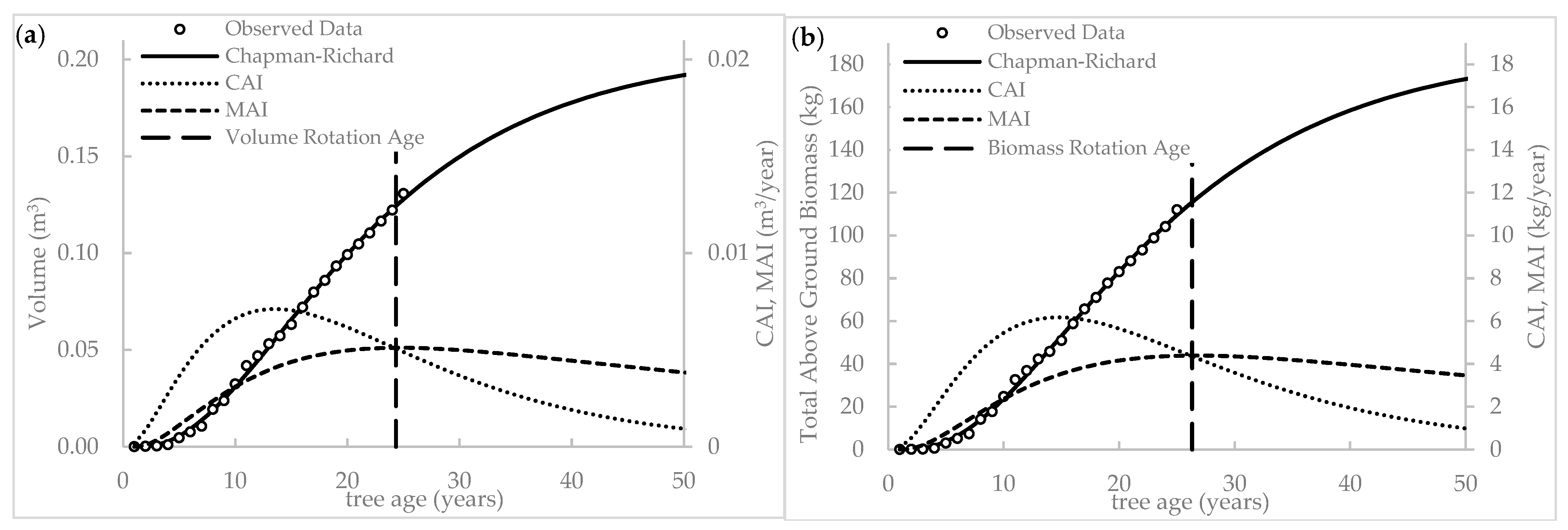
3.3. Biological Rotation Age Prediction

3.3.1. Volume- and Biomass-Based Rotation Age

An allometric equation also generally predicts the tree trunk or clear-bole timber volume. Volume is the function of basal area and height. Substituting the diameter onto the basal area and applying the tree form factor value, the volume can be rewritten as the function of diameter and height. The tree form factor is related to the species and its growing place, and this study chose Hartavia’s [61] report on the community forest teak tree form factor value of 0.44. The plot of volume vs. tree age is presented in Figure 6a, and the Chapman–Richards model fitted the volume growth curve (Equation (19)) with good goodness of fit. The non-linear regression’s coefficient of determination (R²) value is 0.9985, and the mean square error (MSE) is 0.00000338. According to the volume growth curve, the last data are at the end of the linear stage and seem to begin the logarithm stage; the teak specimen was at the end of full-vigor maturity and continued into the early senescent phase. It needed a long time to reach the old phase. The volume growth curve is a fundamental piece of data commonly used for determining the harvesting time of forest trees if the management is aiming to optimize sustainable timber production in the long-term yield.

$$V=0.2049{\left(1-1.0792\mathrm{e}\mathrm{x}\mathrm{p}\left(-0.0762t\right)\right)}^{\frac{1}{1-0.6294}}$$

(19)

If the age unit is year, the first derivation of the growth curve indicates the current annual increment (CAI). Figure 6a shows CAI increases in the juvenile phase and turns to decreasing after full-vigor maturity. The CAI peak, represented by its turning point, coincides with the growth curve’s inflection point, indicating the fastest growth rate. At the growth curve’s inflection point, the second derivation of the growth formula has a zero value. The second derivation of the growth formula equals the first derivation of CAI. Figure 6a also graphs the mean annual increment (MAI), where MAI is the volume growth divided by its current age. The intersection between CAI and MAI determines the biological rotation age and the proposed harvesting time that will obtain the optimum yield of clear bole volume. The CAI is higher than MAI before the biological rotation age; in contrast, the CAI is lower than MAI after that point. Figure 6a shows that the volume-based rotation age of the community teak plantation is 24.3 years. Since the specimen was taken from 220 cm height, where the saplings need approximately 3–4 years to reach that height, the recommended harvesting age is 28 years based on the clear bole volume yield.

Since teak is a versatile usage tree species, where all of its parts may be used, biomass yield may promise another sensible consideration in determining the optimum biological rotation age, in addition to the clear bole volume yield. Applying Purwanto and Silaban’s allometric equation [21] to estimate the community forest’s teak above-ground biomass (AGB), the AGB vs. tree age plot is presented in Figure 6b. The best fit Chapman–Richards model for the biomass growth curve is Equation (20) with R² and MSE values of 0.9986 and 2.3271, respectively. It was derived to obtain CAI and MAI; their intersection is 26.3 years. The biomass-based optimum rotation age is two years older than the volumetric-based one. The proposed harvesting period is 30 years based on the above-ground biomass yield.

$$AGB=187.4830{\left(1-1.0760 \mathrm{e}\mathrm{x}\mathrm{p}\left(-0.0733t\right)\right)}^{\frac{1}{1-0.6482}}$$

(20)

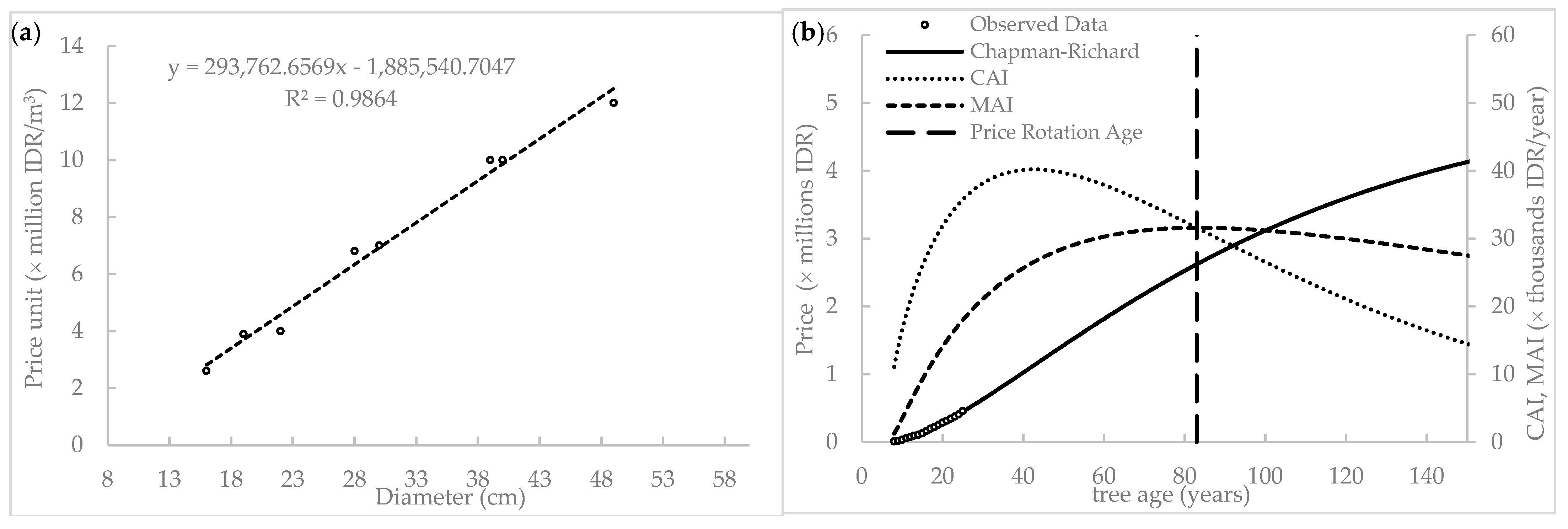
3.3.2. Price-Based Rotation Age

The teak plantation tree may be sold in a stand after reaching nine years old, where the diameter reaches 9–10 cm, when the farmer urgently needs cash. The smaller-diameter trees are not yet salable. The buyer may cut the tree after its diameter reaches more than 16 cm; therefore, about 10 years are needed to harvest the teak tree in this debt bondage transaction. The common normal transaction of a teak tree happens when its diameter is 15–50 cm. The price unit increases with a bigger diameter. The price unit of a 16 cm diameter teak tree is IDR 2,600,000/m³, while the 49 cm diameter is IDR 12,000,000/m³. Figure 7a indicates the linear relationship and strong correlation between diameter and price unit.

By multiplying the price unit and the volume, the price (IDR) of a teak tree related to its age is plotted in Figure 7b. Surprisingly, the plot resembles only the exponential shape part of the sigmoid. It is a different stage than the previous volume- and biomass-based growth curve. The price growth rate of the teak specimen is still accelerated. The non-linear regression based on the Chapman–Richards models to fit the price growth curve resulted in Equation (21) (R² = 0.9987, MSE = 33278801). The price always increases with the tree’s age. Its price increment rate accelerated during the first 40 years and decelerated afterward. The price-based CAI and MAI meet at 83 years old; the harvesting period should be 86 years to obtain the optimum long-term price yield.

$$IDR=5191000{\left(1-1.0939 \mathrm{e}\mathrm{x}\mathrm{p}\left(-0.0144t\right)\right)}^{\frac{1}{1-0.4115}}$$

(21)

The price-based biological rotation age justified that teak plantations keep maintaining their economic benefit for long-term savings. This numerical analysis scientifically confirms the local wisdom of passing down the teak plantation for future generations’ welfare. Villagers planted teak trees as a source of secure prosperity for their descendants and only harvested them when in urgent need. This sociocultural behavior supports the sustainability concept of natural resources, and we must respect it as a good practice exemplified by our ancestors.

4. Discussion

4.1. Community’s Teak Plantation

Teak has been harvested for centuries to produce high-quality, durable, and fancy decorative timber as a raw material for art and jewelry [68], handicraft and wood carving [69,70], carpentry [71], traditional household items [72], furniture [73,74,75,76,77,78,79], architectural buildings and construction [80,81,82], and shipbuilding [83] because of its inherent natural desirable characteristics (i.e., lightweight but high strength and hardness, dimensional stability, natural durability, straight grain and easily woodworking, and beautiful artistic appearance). Teak is a tree species that produces one of the most valuable premium timbers all around the globe. Although hard and strong, teak wood can be cut and machined easily. Its ring-porous anatomical characteristic produces a distinct growth ring and displays an elegant and picturesque pattern on the boards. The heartwood color is yellowish to golden-brown, distinctly different from sapwood’s whitest to pale yellowish-brown color. Fine sanding of the board to a smooth surface displays an innate glossy oily appearance. Older teak trees produce wood with a darker color than the younger ones because of the accumulation of extractive contents. Tectoquinone (β-methyl anthraquinone) extractive, typically deposited in its heartwood, is a toxic substance to decaying fungi, subterranean termites, and dry-wood termites; thus, its concentration is responsible for the high natural durability of the wood [84]. Teak sawn-timber from older trees generally has more desirable characteristics. A bigger diameter log, usually cut from an older tree, is much more expensive than a smaller and younger one.

Besides producing important commercial timber, all parts of a teak tree can be utilized for multiple products. Teak heartwood extractives, barks, and leaves are also locally utilized for ethnobotanical folklore medicine [85] for veterinarians and humans. Teak plants contain phytochemical, pharmacological, and therapeutic potential substances that may be useful for wound healing, as well as having hypoglycemic, cytotoxic, analgesic, antioxidant, anti-inflammatory, antipyretic, and anti-plasmodial activities [86]. The carotenoid extractive substances in teak are beneficial for natural dyes for fabrics [87,88], hair dyes [89], dye-sensitized solar cells [90], and natural pigments for textiles, paints, plastics, foods, drugs, and cosmetics [91]. Villagers also exploited teak wood for energy resources like charcoal [92,93,94,95,96], firewood [97], bio-pellets [98], and bio-briquette [99,100]. Its versatile usage keeps the demand for teak high. Because of its endangered status, teak harvesting in natural forests is banned in its native origin countries (India, Lao PDR, and Thailand) except for Myanmar. Therefore, commercial teak wood available in the market must be logged from plantations.

People in the villages plant teak trees on their private land, in community forests, and even in religious and cultural areas to meet local community and individual needs. It is common to find teak trees in traditional graveyards in Java. The Javanese people have known teak for a long time and value it highly. Villagers inherited their ancestors’ knowledge of the teak silvicultural system and intentionally planted a teak tree as a gift for their future descendants. This good practice of social culture is a strong provision for promoting the concept of sustainability to build cultural value as a strategy to develop ecology-minded design [101]. The traditional community and personal property holders have a high potential to drive the sustainable development of the teak plantations. This study introduces the fundamental aspect of sustainability (i.e., the growth curve of teak’s stem volume, biomass, and price and defining the optimal harvesting periods based on a comprehensive analysis of the annual tree ring) to disseminate it to the community that will enable the development of sustainable teak plantations and their socio-economic value creation.

4.2. Tree Ring Analysis

The vascular cambium differentiation-producing xylem in the rainy and drought seasons yields earlywood and latewood gradation intervals. It generates tree rings that reflect the tree’s biography during the tree growth periods and are beneficial for reconstructing and dating the backward environment circumstances [102,103,104,105,106]. Tree ring studies have recently become a widely interesting topic in interdisciplinary sciences because they may contain signals of individual and environmental conditions providing information concerning many aspects (i.e., biology, hydrology, climatology, geology, and archeology). The vascular cambium differentiation-producing xylem is sensitive to internal and external factors, generating tree ring formation variation. Tree rings may provide information related to the combination of phenotypes–genetics–environments and transcriptomics that potentially decipher the tree’s genomic architecture evolution [107] in adapting to the environmental stress in the competition for survival of the fittest. Tree ring analysis may result in the history of the habitat’s temperature, precipitation, aridity gradients, toxic exposure and pollution, and the individual and population adaptive reactions [108] to those variations. The national repositories might compile the tree ring data sets [109] to provide a library for dendrochronology analysis. A tree may live for hundreds or thousands of years, and the interlinked phenotype–genotype–environment network interpretation from an old tree’s rings significantly enriches our knowledge about past climate (paleoclimatology) and future predictions to prepare for climate change mitigation.

In addition to the long-term benefit of climate change mitigation, tree ring analysis may provide information to obtain the equilibrium of ecological and economic advantages in sustainable forest management. Annual tree rings reflect the tree’s growth and increment; those are fundamental components of knowledge in plant science. The tree rings contain information on tree growth and forest productivity, including its age-related dimension, which is always necessary for sustainable forest management. The next formed tree ring is always larger in diameter and located outside the previous one, which is successfully demonstrated in this study through its elliptical shape idealization. The next year’s tree ring is always outside the previous year.

The vascular cambium is only a single layer of cell called the initial cell. However, distinguishing the initial cell from its still-undifferentiated daughter cells is not easy. Thus, the cambium or cambial zone often denotes the collection of several cell layers originating from undifferentiated cells that retain their embryonic capacity for continued growth and differentiation. Cambial cells produce secondary xylem and secondary phloem. Xylem structure is associated with the age of the vascular cambium. Xylem vessel characteristics, including diameter, length, and porosity, change with the increasing cambial age. Vessel diameter and length increase with increased cambial age [110]. The older cambium produces larger and longer vessels and wider diameter pit membranes. Cambial age negatively correlates with annual diameter growth [111,112]. The outer xylem is produced by the differentiation of an older cambium. During the vascular cambium differentiation to produce xylem formation, the newly formed wood cells attached to the surface of a tree stem’s wood naturally receive tensile stress; they are stretched in the longitudinal direction and compressed in the tangential direction [113]. The tensile stress in the longitudinal direction causes axial elongation and transversal shortening. The ratio of transversal strain to the axial strain is the Poisson ratio. This Poisson-effect phenomenon results in slenderer (longer and thinner) wood cells and a thinner xylem layer in the outer part of the stem than the inner ones. This study’s results are consistent with this phenomenon. The outer tree ring width is generally thinner than the inner one, attributed to the slenderer wood cells in the outer layer.

In addition to inter-layer variation, the tree ring width in a layer also varies. The annual tree ring digitization circumference and its idealized ellipse shape (Figure 1b,c) visually indicate this width variation in a layer. The ellipse shapes are not parallel, and their centers translocate from the pith. The reaction wood formation is suspected to be the cause of this phenomenon. A tree has an innate physiological characteristic to form reaction wood [113] strengthening its structure for long-term survival, responding to genetics [114], environmental [115] and mechanical [116] perturbations, maintaining the vertical alignment [117] of a leaning stem [118] following its gravitropism (geotropism) [119,120] behavior, and driving the primary growth of its stems, branches, or roots toward or away from light (phototropism) [121], water (hydrotropism) [122,123,124,125], heat and temperature changes (thermotropism) [126], and nutrition or toxic chemical substances (chemotropism) [127]. The tree produces reaction wood, in this case, tension wood, because the teak species belongs to Angiospermae, straightening its stem vertically in the opposite direction of gravity. Tension wood is formed on the upper side of a leaning stem, which is typical for angiosperms [62,128,129]. Following the gravitropism habitude, teak trees produce tension wood on the under-tension side of the stem, pulling it towards the affecting load to try to make it vertically straight again. The reaction wood formation produces a wider tree ring on one side than the other, which translocates the stem’s center geometry from the pith. The magnitude of the center translocation is measured using the pith eccentricity. As explicated in this study, the center geometry movement may tell us the history of the stem’s leaning.

The ellipse curve fitting successfully idealized each tree ring and determined its age-related diameter. Diameter is commonly measured as the average of the minimum and maximum values, equal to the average of the minor and major axes. The diameter growth curve can be developed using the average minor and major axes as the dependent variable and the tree ring count number as the indicating predictor. The diameter growth curve is the basic information related to the tree’s other dimensional growth, including the basal area, height, volume, and biomass.

4.3. Growth Curve

As a tree grows, the increase in its size is irreversible. An older tree usually has a bigger diameter, wider basal area, and larger volume; therefore, its dimensions positively correlate to its age. A sigmoid curve, similar to the S alphabet, represents the non-linear function correlation between dimension and age. The growth curve is the graphical appearance of the size (N) vs. age (t) plots and their curve fitting. Verhulst–Pearl [22,23,24,25], Gompertz [26,27,28,29,30,31], von Bertalanffy [32,33,34], and Chapman–Richards [35,36] logistic family formulas are widely known to draw an organism’s (including a tree’s) growth curve. The Verhulst–Pearl logistic curve [66], the most frequently employed growth curve model in the literature, has a fixed inflection point in the middle of the upper and lower asymptotes [130]. The Gompertz [29] usage frequency is second to Verhulst–Pearl’s; it has curve-fitted the growth of plants [131], animals [132,133], and people [134]. The Gompertz is also common for fitting algae [135], bacteria [136], microbe [137,138], and tumor [139,140] growth curves. Verhulst–Pearl, Gompertz, and von Bertalanffy each have three parameters. They are unified and generalized into the Richards family’s four-parameter sigmoid growth model [67].

Since the Chapman–Richards model has an additional parameter, it is more flexible and usually results in a better fit estimation than the three-parameter models. All growth stages (i.e., exponential, linear, logarithm, and asymptotic) are accommodated. The Chapman–Richards growth curve model successfully best fits the teak’s age-related diameter. The annual tree ring’s average minor and major axes present age-related diameters. The option to represent the tree’s age-related diameter by its annual tree ring is the simplification of a more complicated natural phenomenon. The tree diameter enlargement occurs in secondary growth due to the formation of secondary phloem and secondary xylem through the vascular cambium differentiation, plus the cork cambium action forming the tough outermost layer of the stem. Forest mensuration in forest inventory commonly calculates the tree diameter by measuring the outside circumference, including the inner and outer bark. In contrast, the annual tree ring denotes the xylem layer as a part of the secondary vascular tissue added by the vascular cambium. This study’s proposed method to choose the tree’s annual tree ring as the tree’s age-related diameter deviates from the common forest mensuration’s diameter measurement. The estimated diameter derived from the annual tree ring may be systematically smaller than the common measurement. This systematic bias occurs on each tree ring and needs further study to evaluate. This current study neglected the deviation and chose the best-fit growth curve of the annual tree ring diameter to represent the tree’s age-related diameter. The experimentally justified best-fit growth curve, the Chapman–Richards, is further selected to analyze the current annual increment (CAI), mean annual increment (MAI), and biological rotation age.

4.4. Increment and Biological Rotation Age

The Chapman–Richards growth curve model, based on the tree’s diameter, basal area, volume, and biomass, defined that the tree specimen was felled when approximately in between its full-vigor maturity and senescent phase. It could still grow, increasing its dimension, although the velocity was decelerating. Its CAI is still higher than its MAI, indicating its under-age cut. The intersection between CAI and MAI, where the biological rotation age was denoted, was outside the observed data range; therefore, the extrapolation may result in wide bias. However, since the best-fit estimation gave a high confidence level (R² = 0.99), the biological rotation prediction was reasonable and provided the best available estimation on hand.

According to the volume-based biological rotation age, the harvesting period of a community’s teak plantation is 28 years. Meanwhile, the biomass-based one resulted in a slightly longer period, that is, 30 years. These values determine the optimum long-term clear bole volume and above-ground biomass yields in sustainable forest management. A teak plantation’s contribution to the ecological benefit always increases during its lifetime because its cumulative biomass production absorbs CO₂ from the atmosphere. During its lifetime, the leaves may be taken for food wrapping in traditional celebrations or daily packed meals or be used for natural dyes and traditional medicine. Silvicultural treatment, such as pruning, may produce branch and twig cuts for handicraft and energy resources. The multiple usage product of all parts of the teak plantation, even during its lifetime, deters biomass deterioration and lengthens the carbon stock. Therefore, the net carbon sequestration is always positive, even of the old trees, and positively impacts the environment. The cumulative ecological contribution of an older healthy tree is greater than a younger one, especially in community plantations or urban environments where the plantation distances are long.

In addition to the ecological contribution, the socio-economic consideration may act as the main rule for the people or personal property holders deciding to keep, sell, or cut their plantation. This study predicts that the optimum price yield of clear bole logs is approximately 86 years. This result justifies the good sociocultural habitude of villagers to plant the teak as a gift inheritance for their descendants. We disseminate this result to re-encourage people to plant trees, including teak, on their private lands and in community forests and treat it as environmentally friendly long-term wealth. People can enjoy a good life in a green environment while guaranteeing more prosperous future generations.

5. Future Work

This study proposed a mathematical approach as the basis for developing an analysis for further experimental research. The ellipse curve fitting in a polar diagram successfully idealizes the annual tree ring. The teak annual tree rings are clearly seen; therefore, this study did not conduct a deeper anatomical analysis. The idealized ellipse curves also deduce reaction wood formation and location according to its geometric center translocation and approximate the tree-leaning history. Theoretical explication has justified the deduced finding based on the current knowledge and visual observation of a teak disk. Anatomical observation is recommended to validate this mathematical derivation, especially for other tree species whose tree ring is not clearly seen and difficult to observe. Empirical observation of the wood’s anatomy and chemical components may strengthen this finding.

A specimen may be insufficient to represent the population when general statistics are applied. It is widely accepted that the sample size corresponds to the statistical analysis’s confidence level. This study exemplified a deep analysis of a single disk specimen based on custom statistics models, where the theoretical basis was first stated. Then, the mathematical models were developed based on these theoretical statements. The statistical analysis procedure was conducted to fit the mathematical model, resulting in the theoretical-based deduction and minimizing the data-driven inductive estimation. The theoretical-based custom statistical model may significantly reduce the minimum sampling size requirement to acquire the targeted confidence level. However, a larger sampling will always give a better confidence level. Therefore, we propose more representative sampling for future work. This study introduced the potential for further work and analysis.

6. Conclusions

This study applied an elliptical polar form of non-linear regression to curve fit the annual tree ring of a teak disk specimen and determine its age-related diameter and basal area. Based on the tree ring’s estimated diameter, the allometric equations estimated the above-ground biomass and clear-bole volume. The continuous growth formula and the discrete ones fitted the growth curve with good goodness of fit, and this study found that Chapman–Richards is the best fit among others. The growth curve, current annual increment (CAI), and mean annual increment (MAI) were graphed based on the clear-bole volume, above-ground biomass, and log timber price; the CAI and MAI intersections result in 28, 30, and 86 years of optimum harvesting period, respectively. These results confirm that the teak plantation is a sustainable and highly valuable asset to inherit with long-term positive benefits for descendants. The sociocultural provision of teak plants as an inheritance gift for the next generation has been justified as beneficial in supporting the sustainability of natural resources.

References

1. Gua, B.; Pedersen, A.; Barstow, M. Tectona Grandis. The IUCN Red List of Threatened Species 2022: E.T62019830A62019832. Available online: https://www.iucnredlist.org/species/62019830/62019832#assessment-information (accessed on 25 June 2023).
2. Budiono, R.; Nugroho, B.; Hardjanto; Nurrochmat, D.R. Dinamika Hegemoni Penguasaan Hutan Di Indonesia (The Dynamics of Forest Hegemony in Indonesia). J. Anal. Kebijak. Kehutan. 2018, 15, 113–125. [Google Scholar] [CrossRef]
3. Nugroho, H.Y.S.H.; Indrajaya, Y.; Astana, S.; Murniati; Suharti, S.; Basuki, T.M.; Yuwati, T.W.; Putra, P.B.; Narendra, B.H.; Abdulah, L.; et al. A Chronicle of Indonesia’s Forest Management: A Long Step towards Environmental Sustainability and Community Welfare. Land 2023, 12, 1238. [Google Scholar] [CrossRef]
4. Peluso, N.L. The History of State Forest Management in Colonial Java. For. Conserv. Hist. 1991, 35, 65–75. [Google Scholar] [CrossRef]
5. Boomgaard, P. Forest Management and Exploitation in Colonial Java, 1677–1897. For. Conserv. Hist. 1992, 36, 4–14. [Google Scholar] [CrossRef]
6. Moore, J.E.; Mascarenhas, A.; Bain, J.; Straus, S.E. Developing a Comprehensive Definition of Sustainability. Implement. Sci. 2017, 12, 110. [Google Scholar] [CrossRef]
7. Mukherjee, A.; Kamarulzaman, N.H.; Vijayan, G.; Vaiappuri, S.K.N. Sustainability: A Comprehensive Literature. In Handbook of Research on Global Supply Chain Management; Christiansen, B., Ed.; IGI Global: Hershey, PA, USA, 2016; pp. 248–268. ISBN 9781466696402. [Google Scholar]
8. Gaitan-Alvarez, J.; Moya, R.; Berrocal, A. The Use of X-ray Densitometry to Evaluate the Wood Density Profile of Tectona Grandis Trees Growing in Fast-Growth Plantations. Dendrochronologia 2019, 55, 71–79. [Google Scholar] [CrossRef]
9. Patel, V.R.; Pramod, S.; Rao, K.S. Cambial Activity, Annual Rhythm of Xylem Production in Relation to Phenology and Climatic Factors and Lignification Pattern during Xylogenesis in Drum-Stick Tree (Moringa oleifera). Flora-Morphol. Distrib. Funct. Ecol. Plants 2014, 209, 556–566. [Google Scholar] [CrossRef]
10. Buajan, S.; Songtrirat, P.; Muangsong, C. Relationship of Cambial Activity and Xylem Production in Teak (Tectona Grandis) to Phenology and Climatic Variables in North-Western Thailand. J. Trop. For. Sci. 2023, 35, 141–156. [Google Scholar] [CrossRef]
11. Karlinasari, L.; Bahtiar, E.T.; Kadir, A.S.A.; Adzkia, U.; Nugroho, N.; Siregar, I.Z. Structural Analysis of Self-Weight Loading Standing Trees to Determine Its Critical Buckling Height. Sustainability 2023, 15, 6075. [Google Scholar] [CrossRef]
12. Dargahi, M.; Newson, T.; Moore, J. Buckling Behaviour of Trees under Self-Weight Loading. For. An Int. J. For. Res. 2019, 92, 393–405. [Google Scholar] [CrossRef]
13. Leblicq, T.; Vanmaercke, S.; Ramon, H.; Saeys, W. Mechanical Analysis of the Bending Behaviour of Plant Stems. Biosyst. Eng. 2015, 129, 87–99. [Google Scholar] [CrossRef]
14. Spatz, H.-C.; Bruechert, F. Basic Biomechanics of Self-Supporting Plants: Wind Loads and Gravitational Loads on a Norway Spruce Tree. For. Ecol. Manag. 2000, 135, 33–44. [Google Scholar] [CrossRef]
15. Huang, Y.-S.; Hsu, F.-L.; Lee, C.-M.; Juang, J.-Y. Failure Mechanism of Hollow Tree Trunks Due to Cross-Sectional Flattening. R. Soc. Open Sci. 2017, 4, 160972. [Google Scholar] [CrossRef]
16. Bahtiar, E.T. Kekuatan Material: Teori, Contoh Kasus, Dan Penyelesaian, 1st ed.; Gumelar, A.D., Ed.; Penerbit IPB Press: Bogor, Indonesia, 2018; ISBN 978-602-440-576-2. [Google Scholar]
17. Timoshenko, S. Strength of Materials. Nature 1942, 150, 645. [Google Scholar] [CrossRef]
18. Akachuku, A.E.; Abolarin, D.A.O. Variations in Pith Eccentricity and Ring Width in Teak (Tectona grandis L. F.). Trees 1989, 3, 111–116. [Google Scholar] [CrossRef]
19. Venugopal, N.; Khrisnamurthy, K.V. Seasonal Production of Secondary Phloem in the Twigs of Certain Tropical Timber Trees. Ann. Bot. 1987, 60, 61–67. [Google Scholar] [CrossRef]
20. Denih, A.; Putra, G.R.; Kurniawan, Z.; Bahtiar, E.T. Developing a Model for Curve-Fitting a Tree Stem’s Cross-Sectional Shape and Sapwood–Heartwood Transition in a Polar Diagram System Using Nonlinear Regression. Forests 2023, 14, 1102. [Google Scholar] [CrossRef]
21. Purwanto, R.H.; Silaban, M. Inventore Biomasa Dan Karbon Jenis Jati (Tectona grandis L.f.) Di Hutan Rakyat Desa Jatimulyo, Karanganyar. J. Ilmu Kehutan. 2011, 5, 40–50. [Google Scholar] [CrossRef]
22. Samawal, M. Thoughts and Rectifications for Verhulst Growth Model: A Scientific Mathematization for a General Theory of Growth Led to a Fundamental Law of Growth. SSRN Electron. J. 2023. [CrossRef]
23. Gatto, M.; Muratori, S.; Rinaldi, S. A Functional Interpretation of the Logistic Equation. Ecol. Modell. 1988, 42, 155–159. [Google Scholar] [CrossRef]
24. Verhulst, P.F. Recherches Mathématiques Sur La Loi d’accroissement de La Population; Nouveaux Mémoires de l’Académie Royale des Sciences et Belles-Lettres de Bruxelles: Bruxelles, Belgium, 1820; pp. 1–40. [Google Scholar]
25. David, H.A.; Edwards, A.W.F. The Logistic Growth Curve. In Annotated Readings in the History of Statistics. Springer Series in Statistics; Springer: New York, NY, USA, 2001; pp. 65–67. [Google Scholar]
26. Gompertz, B. On the Nature of the Function Expressive of the Law of Human Mortality, and on a New Mode of Determining the Value of Life Contingencies. In a Letter to Francis Baily, Esq. F. R. S. &C. Philos. Trans. R. Soc. London 1825, 115, 513–583. [Google Scholar] [CrossRef]
27. Kyurkchiev, V.; Iliev, A.; Rahnev, A.; Kyurkchiev, N. On a Piecewise Smooth Gompertz Growth Function. Applications. In Proceedings of the New Trends in the Applications of Differential Equations in Sciences, Sozopol, Bulgaria, 14–17 June 2022; NTADES 2022; Springer Proceedings in Mathematics & Statistics. Slavova, A., Ed.; Springer: Cham, Switzerland, 2022; Volume 412, pp. 461–472. [Google Scholar]
28. Fang, S.-L.; Kuo, Y.-H.; Kang, L.; Chen, C.-C.; Hsieh, C.-Y.; Yao, M.-H.; Kuo, B.-J. Using Sigmoid Growth Models to Simulate Greenhouse Tomato Growth and Development. Horticulturae 2022, 8, 1021. [Google Scholar] [CrossRef]
29. Tjørve, K.M.C.; Tjørve, E. The Use of Gompertz Models in Growth Analyses, and New Gompertz-Model Approach: An Addition to the Unified-Richards Family. PLoS ONE 2017, 12, e0178691. [Google Scholar] [CrossRef] [PubMed]
30. Estrada, E.; Bartesaghi, P. From Networked SIS Model to the Gompertz Function. Appl. Math. Comput. 2022, 419, 126882. [Google Scholar] [CrossRef]
31. Gultom, F.R.P.; Solimun, S.; Nurjannah, N. Bootstrap Resampling in Gompertz Growth Model with Levenberg–Marquardt Iteration. JTAM (Jurnal Teor. Apl. Mat.) 2022, 6, 810. [Google Scholar] [CrossRef]
32. Lee, L.; Atkinson, D.; Hirst, A.G.; Cornell, S.J. A New Framework for Growth Curve Fitting Based on the von Bertalanffy Growth Function. Sci. Rep. 2020, 10, 7953. [Google Scholar] [CrossRef]
33. Croll, J.C.; van Kooten, T. Accounting for Temporal and Individual Variation in the Estimation of Von Bertalanffy Growth Curves. Ecol. Evol. 2022, 12, e9619. [Google Scholar] [CrossRef]
34. von Bertalanffy, L. Quantitative Laws in Metabolism and Growth. Q. Rev. Biol. 1957, 32, 217–231. [Google Scholar] [CrossRef]
35. Simpson, M.J.; Browning, A.P.; Warne, D.J.; Maclaren, O.J.; Baker, R.E. Parameter Identifiability and Model Selection for Sigmoid Population Growth Models. J. Theor. Biol. 2022, 535, 110998. [Google Scholar] [CrossRef]
36. Jannatizadeh, A.; Rezaei, M.; Rohani, A.; Lawson, S.; Fatahi, R. Towards Modeling Growth of Apricot Fruit: Finding a Proper Growth Model. Hortic. Environ. Biotechnol. 2023, 64, 209–222. [Google Scholar] [CrossRef]
37. Bahtiar, E.T.; Darwis, A. Exponential Curve Modification by Linear and Nonlinear Function to Fit the Fiber Length of Teakwood (Tectona Grandis). J. Biol. Sci. 2014, 14, 183–194. [Google Scholar] [CrossRef]
38. Cahyono, T.D.; Wahyudi, I.; Priadi, T.; Febrianto, F.; Darmawan, W.; Bahtiar, E.T.; Ohorella, S.; Novriyanti, E. The Quality of 8 and 10 Years Old Samama Wood (Anthocephalus macrophyllus). J. Indian Acad. Wood Sci. 2015, 12, 22–28. [Google Scholar] [CrossRef]
39. Ferrero, M.E.; Villalba, R.; Rivera, S.M. An Assessment of Growth Ring Identification in Subtropical Forests from Northwestern Argentina. Dendrochronologia 2014, 32, 113–119. [Google Scholar] [CrossRef]
40. Kanzow, C.; Yamashita, N.; Fukushima, M. Levenberg–Marquardt Methods with Strong Local Convergence Properties for Solving Nonlinear Equations with Convex Constraints. J. Comput. Appl. Math. 2004, 172, 375–397. [Google Scholar] [CrossRef]
41. Levenberg, K. A Method for the Solution of Certain Non-Linear Problems in Least Squares. Q. Appl. Math. 1944, 2, 164–168. [Google Scholar] [CrossRef]
42. Lourakis, M.I.A. A Brief Description of the Levenberg-Marquardt Algorithm Implemened by Levmar; Heraklion: Crete, Greece, 2005. [Google Scholar]
43. Firmanti, A.; Bachtiar, E.T.; Surjokusumo, S.; Komatsu, K.; Kawai, S. Mechanical Stress Grading of Tropical Timbers without Regard to Species. J. Wood Sci. 2005, 51, 339–347. [Google Scholar] [CrossRef]
44. Bahtiar, E.T.; Trujillo, D.; Nugroho, N. Compression Resistance of Short Members as the Basis for Structural Grading of Guadua Angustifolia. Constr. Build. Mater. 2020, 249, 118759. [Google Scholar] [CrossRef]
45. Bahtiar, E.T.; Imanullah, A.P.; Hermawan, D.; Nugroho, N. Abdurachman Structural Grading of Three Sympodial Bamboo Culms (Hitam, Andong, and Tali) Subjected to Axial Compressive Load. Eng. Struct. 2019, 181, 233–245. [Google Scholar] [CrossRef]
46. Bahtiar, E.T.; Nugroho, N.; Rahman, M.M.; Arinana; Kartika Sari, R.; Wirawan, W.; Hermawan, D. Estimation the Remaining Service-Lifetime of Wooden Structure of Geothermal Cooling Tower. Case Stud. Constr. Mater. 2017, 6, 91–102. [Google Scholar] [CrossRef]
47. Nugroho, N.; Bahtiar, E.T. Nurmadina Grading Development of Indonesian Bamboo Culm: Case Study on Tali Bamboo (Gigantochloa apus). In Proceedings of the 2018 World Conference on TImber Engineering, Seoul, Republic of Korea, 20–23 August 2018; pp. 1–6. [Google Scholar]
48. Bahtiar, E.T.; Denih, A.; Putra, G.R. Multi-Culm Bamboo Composites as Sustainable Materials for Green Constructions: Section Properties and Column Behavior. Results Eng. 2023, 17, 100911. [Google Scholar] [CrossRef]
49. Sylvayanti, S.P.; Nugroho, N.; Bahtiar, E.T. Bamboo Scrimber’s Physical and Mechanical Properties in Comparison to Four Structural Timber Species. Forests 2023, 14, 146. [Google Scholar] [CrossRef]
50. Cahyono, T.D.; Wahyudi, I.; Priadi, T.; Febrianto, F.; Bahtiar, E.T.; Novriyanti, E. Analysis on Wood Quality, Geometry Factor, and Their Effects on Lathe Check of Samama (Anthocephalus macrophyllus) Veneer. J. Korean Wood Sci. Technol. 2016, 44, 828–841. [Google Scholar] [CrossRef]
51. Nugroho, N.; Kartini; Bahtiar, E.T. Cross-Species Bamboo Grading Based on Flexural Properties. IOP Conf. Ser. Earth Environ. Sci. 2021, 891, 012008. [Google Scholar] [CrossRef]
52. Nurmadina; Nugroho, N.; Bahtiar, E.T. Structural Grading of Gigantochloa Apus Bamboo Based on Its Flexural Properties. Constr. Build. Mater. 2017, 157, 1173–1189. [Google Scholar] [CrossRef]
53. Darwis, A.; Nurrochmat, D.R.; Massijaya, M.Y.; Nugroho, N.; Alamsyah, E.M.; Bahtiar, E.T.; Safei, R. Vascular Bundle Distribution Effect on Density and Mechanical Properties of Oil Palm Trunk. Asian J. Plant Sci. 2013, 12, 208–213. [Google Scholar] [CrossRef]
54. Arinana; Philippine, I.; Koesmaryono, Y.; Nandika, D.; Rauf, A.; Harahap, I.S.; Sumertajaya, I.M.; Bahtiar, E.T. Coptotermes Curvignathus Holmgren (Isoptera: Rhinotermitidae) Capability to Maintain the Temperature Inside Its Nests. J. Entomol. 2016, 13, 199–202. [Google Scholar] [CrossRef]
55. Bahtiar, E.T.; Erizal, E.; Hermawan, D.; Nugroho, N.; Hidayatullah, R. Experimental Study of Beam Stability Factor of Sawn Lumber Subjected to Concentrated Bending Loads at Several Points. Forests 2022, 13, 1480. [Google Scholar] [CrossRef]
56. Bahtiar, E.T.; Arinana; Nugroho, N.; Nandika, D. Daily Cycle of Air Temperature and Relative Humidity Effect to Creep Deflection of Wood Component of Low-Cost House in Cibeureum-Bogor, West Java, Indonesia. Asian J. Sci. Res. 2014, 7, 501–512. [Google Scholar] [CrossRef]
57. Bahtiar, E.T.; Nugroho, N.; Karlinasari, L.; Surjokusumo, S. Human Comfort Period Outside and Inside Bamboo Stands. J. Environ. Sci. Technol. 2014, 7, 245–265. [Google Scholar] [CrossRef]
58. Nugroho, N.; Bahtiar, E.T. Buckling Formulas for Designing a Column with Gigantochloa Apus. Case Stud. Constr. Mater. 2021, 14, e00516. [Google Scholar] [CrossRef]
59. Bahtiar, E.T.; Malkowska, D.; Trujillo, D.; Nugroho, N. Experimental Study on Buckling Resistance of Guadua Angustifolia Bamboo Column. Eng. Struct. 2021, 228, 111548. [Google Scholar] [CrossRef]
60. Hermawan, D.; Budiman, I.; Febrianto, F.; Subyakto, S.; Pari, G.; Ghozali, M.; Bahtiar, E.T.; Sutiawan, J.; Azevedo, A.R.G. de Enhancement of the Mechanical, Self-Healing and Pollutant Adsorption Properties of Mortar Reinforced with Empty Fruit Bunches and Shell Chars of Oil Palm. Polymers 2022, 14, 410. [Google Scholar] [CrossRef] [PubMed]
61. Hartavia, E. Pemodelan Volume Batang Tegakan Jati Umur 9-13 Tahun Untuk Penaksiran Potensi Hutan Rakyat Di Kabupaten Pati. Ph.D. Thesis, Gadjah Mada University, Yogyakarta, Indonesia, 2019. [Google Scholar]
62. Du, S.; Yamamoto, F. An Overview of the Biology of Reaction Wood Formation. J. Integr. Plant Biol. 2007, 49, 131–143. [Google Scholar] [CrossRef]
63. Bahtiar, E.T.; Iswanto, A.H. Annual Tree-Ring Curve-Fitting for Graphing the Growth Curve and Determining the Increment and Cutting Cycle Period of Sungkai (Peronema canescens). Forests 2023, 14, 1643. [Google Scholar] [CrossRef]
64. Zhao-gang, L.; Feng-ri, L. The Generalized Chapman-Richards Function and Applications to Tree and Stand Growth. J. For. Res. 2003, 14, 19–26. [Google Scholar] [CrossRef]
65. Shifley, S.R.; Brand, G.J. Chapman-Richards Growth Function Constrained for Maximum Tree Size. For. Sci. 1984, 30, 1066–1070. [Google Scholar] [CrossRef]
66. Verhulst, P.-F. Notice Sur La Loi Que La Population Suit Dans Son Accroissement. Corresp. Math. Phys. 1838, 10, 113–129. [Google Scholar]
67. Tjørve, E.; Tjørve, K.M.C. A Unified Approach to the Richards-Model Family for Use in Growth Analyses: Why We Need Only Two Model Forms. J. Theor. Biol. 2010, 267, 417–425. [Google Scholar] [CrossRef]
68. Atherton, C. Simple Jewelry-Silver Bound Boxes. Des. Stud. 1927, 29, 185–188. [Google Scholar]
69. Tiwari, A.K. Bastar Handicrafts: The Visible Cultural Symbol of Bastar Region of Chhattisgarh. Int. J. Res. Humanit. Arts Lit. 2015, 3, 43–48. [Google Scholar]
70. Udaykumar, S. Initial Exploration of the Woodcraft Techniques of Tamil Nadu. Wood Is Good Grow More Use More 2021, 1, 47–50. [Google Scholar]
71. Dumarçay, J. Wood and Carpentry. In Construction Techniques in South and Southeast Asia; BRILL: Leiden, The Netherlands, 2005; pp. 21–35. [Google Scholar]
72. Lookose, S. Traditional Teak Wood Articles Used in Households of Nilambur and Malapuram Areas of Kerala. Indian J. Tradit. Knowl. 2008, 7, 108–111. [Google Scholar]
73. Kongprasert, N. Emotional Design Approach to Design Teak Wood Furniture. In Proceedings of the Asia Pacific Industrial Engineering & Management Systems Conference 2012, Phuket, Thailand, 2–5 December 2012; Kachitvichyanukul, V., Luong, H.T., Pitakaso, R., Eds.; pp. 805–812. [Google Scholar]
74. Chen, T.L.; Hong, P.F. Study on the Visual Image of Armchairs Furniture in Yangming Shu Wu. Adv. Mater. Res. 2010, 168–170, 2371–2375. [Google Scholar] [CrossRef]
75. Puspita, A.A.; Sachari, A.; Sriwarno, A.B. Design Adaptation of Wooden Furniture through Sustainability Design Strategy (Case Studies: Five Furniture Industries in Central Java, Indonesia). Arts Des. Stud. 2016, 45, 1–13. [Google Scholar]
76. Siahaan, H.; Wahyudi, I. Keragaan Permesinan Dan Keteguhan Rekat Kayu Jati Cepat Tumbuh Terdensifikasi. J. Ilmu Pertan. Indones. 2020, 26, 1–7. [Google Scholar] [CrossRef]
77. Suranto, Y. Effect of Breeding Technology and Trunk Axial Position on Shrinkage and Quality of 10 Year Old Teak Wood as a Furniture’s Raw Material. IOP Conf. Ser. Mater. Sci. Eng. 2020, 935, 012037. [Google Scholar] [CrossRef]
78. Afiyah, S.N.; Syaifuddin, M.; Aqromi, N.L. Optimization of Teak Wood Furniture Production Using Linear Programming Method at Sumenep East Java Indonesia. Numer. J. Mat. Pendidik. Mat. 2022, 6, 13–24. [Google Scholar] [CrossRef]
79. Sushardi; Prayitno, T.A.; Suranto, Y.; Lukmandaru, G. Distribution of Certified Wood Teak Wood Machining Properties as Export Furniture Materials. Hutan Trop. 2022, 16, 15–25. [Google Scholar] [CrossRef]
80. Rani, M.F.B.A.; Daud, P.S.D.S.N.I.M. The Role of Wood in Current Sustainable Building in Thailand as Architectural Ornaments. In The Importance of Wood and Timber in Sustainable Buildings; Springer: Berlin/Heidelberg, Germany, 2022; pp. 19–47. [Google Scholar]
81. Christian, R.R. Challenges of Teak Architecture Conservation in Myanmar; Architectural Conservation Working Paper Series; Architectural Conservation: Singapore, 2020. [Google Scholar]
82. Prajwal, S.; Akashaya Kumar, V.H.; Patil, N.N. Implementation of Sustainable Materials in an Existing Residential Building and Comparison. IOP Conf. Ser. Mater. Sci. Eng. 2021, 1166, 012038. [Google Scholar] [CrossRef]
83. Tripati, S.; Shukla, S.R.; Shashikala, S.; Sardar, A. Role of Teak and Other Hardwoods in Shipbuilding as Evidenced from Literature and Shipwrecks. Curr. Sci. 2016, 111, 1262–1268. [Google Scholar]
84. Rudman, P.; Da Costa, E.W.B.; Gay, F.J.; Wetherly, A.H. Relationship of Tectoquinone to Durability in Tectona Grandis. Nature 1958, 181, 721–722. [Google Scholar] [CrossRef]
85. Singh, R.; Verma, K.K.; Choudhary, A.; Veena, S. Screening of Heartwood of Tectona Grandis Linn for Antifungal Activity. Samriddhi A J. Phys. Sci. Eng. Technol. 2021, 13, 111–114. [Google Scholar] [CrossRef]
86. Vyas, P.; Yadav, D.K.; Khandelwal, P. Tectona Grandis (Teak)—A Review on Its Phytochemical and Therapeutic Potential. Nat. Prod. Res. 2019, 33, 2338–2354. [Google Scholar] [CrossRef]
87. Agrawal, A.; Chopra, S. Sustainable Dyeing of Selected Natural and Synthetic Fabrics Using Waste Teak Leaves (Tectona grandis L.). Res. J. Text. Appar. 2020, 24, 357–374. [Google Scholar] [CrossRef]
88. Qadariyah, L.; Mahfud, M.; Sulistiawati, E.; Swastika, P. Natural Dye Extraction From Teak Leaves (Tectona grandis) Using Ultrasound Assisted Extraction Method for Dyeing on Cotton Fabric. MATEC Web Conf. 2018, 156, 05004. [Google Scholar] [CrossRef]
89. Tibkawin, N.; Suphrom, N.; Nuengchamnong, N.; Khorana, N.; Charoensit, P. Utilisation of Tectona Grandis (Teak) Leaf Extracts as Natural Hair Dyes. Color. Technol. 2022, 138, 355–367. [Google Scholar] [CrossRef]
90. Alamu, Q.A.; Adara, P.P.; Kofoworola, A.M.; Oyeshola, H.O. Utilization of Extracted Natural Dye from Tectona Grandis (Teak) as a Sensitizer for Dye-Sensitized Solar Cell. Int. J. Sci. Adv. 2022, 3, 577–580. [Google Scholar] [CrossRef]
91. Charoensit, P.; Sawasdipol, F.; Tibkawin, N.; Suphrom, N.; Khorana, N. Development of Natural Pigments from Tectona Grandis (Teak) Leaves: Agricultural Waste Material from Teak Plantations. Sustain. Chem. Pharm. 2021, 19, 100365. [Google Scholar] [CrossRef]
92. Haryanto, A.; Hidayat, W.; Hasanudin, U.; Iryani, D.A.; Kim, S.; Lee, S.; Yoo, J. Valorization of Indonesian Wood Wastes through Pyrolysis: A Review. Energies 2021, 14, 1407. [Google Scholar] [CrossRef]
93. Siabi, W.K.; Owusu-Ansah, E.D.-J.; Essandoh, H.M.K.; Asiedu, N.Y. Modelling the Adsorption of Iron and Manganese by Activated Carbon from Teak and Shea Charcoal for Continuous Low Flow. Water-Energy Nexus 2021, 4, 88–94. [Google Scholar] [CrossRef]
94. Berrocal-Mendéz, N.; Moya, R. Production, Cost and Properties of Charcoal Produced after Logging and Sawing, by the Earth Pit Method from Tectona Grandis Wood Residues. J. Indian Acad. Wood Sci. 2022, 19, 121–132. [Google Scholar] [CrossRef]
95. Ratnani, R.D.; Purbacaraka, F.H.; Hartati, I.; Syafaat, I. Actived Carbon from Teak Wood, Jackfruit Wood, and Mango Wood Pyrolysis Process. J. Phys. Conf. Ser. 2019, 1217, 012055. [Google Scholar] [CrossRef]
96. Kongnine, D.M.; Kpelou, P.; Attah, N.; Kombate, S.; Mouzou, E.; Djeteli, G.; Napo, K. Energy Resource of Charcoals Derived from Some Tropical Fruits Nuts Shells. Int. J. Renew. Energy Dev. 2020, 9, 29–35. [Google Scholar] [CrossRef]
97. Siarudin, M.; Awang, S.A.; Sadono, R.; Suryanto, P. Renewable Energy from Secondary Wood Products Contributes to Local Green Development: The Case of Small-Scale Privately Owned Forests in Ciamis Regency, Indonesia. Energy. Sustain. Soc. 2023, 13, 4. [Google Scholar] [CrossRef] [PubMed]
98. Iskandar, N.; Sulardjaka, S.; Munadi, M.; Nugroho, S.; Nidhom, A.S.; Fitriyana, D.F. The Characteristic of Bio-Pellet Made from Teak Wood Waste Due to the Influence of Variations in Material Composition and Compaction Pressure. J. Phys. Conf. Ser. 2020, 1517, 012017. [Google Scholar] [CrossRef]
99. Wahyuni, H.; Aladin, A.; Kalla, R.; Nouman, M.; Ardimas, A.; Chowdhury, M.S. Utilization of Industrial Flour Waste as Biobriquette Adhesive: Application on Pyrolysis Biobriquette Sawdust Red Teak Wood. Int. J. Hydrol. Environ. Sustain. 2022, 1, 54–69. [Google Scholar] [CrossRef]
100. Faisal, R.M.; Ardian, A.; Khoiriyah, V.; Chafidz, A. Production of Briquettes from a Blend of HDPE (High Density Polyethylene) Plastic Wastes and Teak (Tectona grandis Linn. f) Sawdust Using Different Natural Adhesives as the Binder. Key Eng. Mater. 2021, 882, 273–279. [Google Scholar] [CrossRef]
101. Puspita, A.A.; Sachari, A.; Sriwarno, A.B. Jamaludin Knowledge from Javanese Cultural Heritage: How They Manage and Sustain Teak Wood. Cultura 2018, 15, 23–48. [Google Scholar] [CrossRef]
102. Decuyper, M.; Chávez, R.O.; Čufar, K.; Estay, S.A.; Clevers, J.G.P.W.; Prislan, P.; Gričar, J.; Črepinšek, Z.; Merela, M.; de Luis, M.; et al. Spatio-Temporal Assessment of Beech Growth in Relation to Climate Extremes in Slovenia—An Integrated Approach Using Remote Sensing and Tree-Ring Data. Agric. For. Meteorol. 2020, 287, 107925. [Google Scholar] [CrossRef]
103. Wang, Z.; Lyu, L.; Liu, W.; Liang, H.; Huang, J.; Zhang, Q.-B. Topographic Patterns of Forest Decline as Detected from Tree Rings and NDVI. Catena 2021, 198, 105011. [Google Scholar] [CrossRef]
104. Bumann, E.; Awada, T.; Wardlow, B.; Hayes, M.; Okalebo, J.; Helzer, C.; Mazis, A.; Hiller, J.; Cherubini, P. Assessing Responses of Betula Papyrifera to Climate Variability in a Remnant Population along the Niobrara River Valley in Nebraska, U.S.A., through Dendroecological and Remote-Sensing Techniques. Can. J. For. Res. 2019, 49, 423–433. [Google Scholar] [CrossRef]
105. Anderson-Teixeira, K.J.; Herrmann, V.; Rollinson, C.R.; Gonzalez, B.; Gonzalez-Akre, E.B.; Pederson, N.; Alexander, M.R.; Allen, C.D.; Alfaro-Sánchez, R.; Awada, T.; et al. Joint Effects of Climate, Tree Size, and Year on Annual Tree Growth Derived from Tree-ring Records of Ten Globally Distributed Forests. Glob. Chang. Biol. 2022, 28, 245–266. [Google Scholar] [CrossRef] [PubMed]
106. Sevik, H.; Cetin, M.; Ozel, H.B.; Akarsu, H.; Zeren Cetin, I. Analyzing of Usability of Tree-Rings as Biomonitors for Monitoring Heavy Metal Accumulation in the Atmosphere in Urban Area: A Case Study of Cedar Tree (Cedrus Sp.). Environ. Monit. Assess. 2020, 192, 23. [Google Scholar] [CrossRef] [PubMed]
107. Depardieu, C.; Gérardi, S.; Nadeau, S.; Parent, G.J.; Mackay, J.; Lenz, P.; Lamothe, M.; Girardin, M.P.; Bousquet, J.; Isabel, N. Connecting Tree-ring Phenotypes, Genetic Associations and Transcriptomics to Decipher the Genomic Architecture of Drought Adaptation in a Widespread Conifer. Mol. Ecol. 2021, 30, 3898–3917. [Google Scholar] [CrossRef]
108. Housset, J.M.; Tóth, E.G.; Girardin, M.P.; Tremblay, F.; Motta, R.; Bergeron, Y.; Carcaillet, C. Tree-Rings, Genetics and the Environment: Complex Interactions at the Rear Edge of Species Distribution Range. Dendrochronologia 2021, 69, 125863. [Google Scholar] [CrossRef]
109. Girardin, M.P.; Guo, X.J.; Metsaranta, J.; Gervais, D.; Campbell, E.; Arsenault, A.; Isaac-Renton, M.; Harvey, J.E.; Bhatti, J.; Hogg, E.H. A National Tree-Ring Data Repository for Canadian Forests (CFS-TRenD): Structure, Synthesis, and Applications. Environ. Rev. 2021, 29, 225–241. [Google Scholar] [CrossRef]
110. Rodriguez-Zaccaro, F.D.; Valdovinos-Ayala, J.; Percolla, M.I.; Venturas, M.D.; Pratt, R.B.; Jacobsen, A.L. Wood Structure and Function Change with Maturity: Age of the Vascular Cambium Is Associated with Xylem Changes in Current-Year Growth. Plant. Cell Environ. 2019, 42, 1816–1831. [Google Scholar] [CrossRef]
111. Ivković, M.; Gapare, W.; Wu, H.; Espinoza, S.; Rozenberg, P. Influence of Cambial Age and Climate on Ring Width and Wood Density in Pinus Radiata Families. Ann. For. Sci. 2013, 70, 525–534. [Google Scholar] [CrossRef]
112. Xiang, W.; Leitch, M.; Auty, D.; Duchateau, E.; Achim, A. Radial Trends in Black Spruce Wood Density Can Show an Age- and Growth-Related Decline. Ann. For. Sci. 2014, 71, 603–615. [Google Scholar] [CrossRef]
113. Plomion, C.; Leprovost, G.; Stokes, A. Wood Formation in Trees. Plant Physiol. 2001, 127, 1513–1523. [Google Scholar] [CrossRef]
114. Ko, J.-H.; Kim, W.-C.; Keathley, D.E.; Han, K.-H. Genetic Engineering for Secondary Xylem Modification: Unraveling the Genetic Regulation of Wood Formation. In Secondary Xylem Biology; Elsevier: Amsterdam, The Netherlands, 2016; pp. 193–211. [Google Scholar]
115. Kozlowski, T.T.; Pallardy, S.G. Environmental Regulation of Vegetative Growth. In Growth Control in Woody Plants; Elsevier: Amsterdam, The Netherlands, 1997; pp. 195–322. [Google Scholar]
116. Telewski, F.W. Flexure Wood: Mechanical Stress Induced Secondary Xylem Formation. In Secondary Xylem Biology; Elsevier: Amsterdam, The Netherlands, 2016; pp. 73–91. [Google Scholar]
117. Wheeler, E. Wood: Macroscopic Anatomy. In Encyclopedia of Materials: Science and Technology; Elsevier: Amsterdam, The Netherlands, 2001; pp. 9653–9657. [Google Scholar]
118. Donaldson, L.; Nanayakkara, B.; Harrington, J. Wood Growth and Development. In Encyclopedia of Applied Plant Sciences; Elsevier: Amsterdam, The Netherlands, 2017; pp. 203–210. [Google Scholar]
119. Gerttula, S.; Zinkgraf, M.; Muday, G.K.; Lewis, D.R.; Ibatullin, F.M.; Brumer, H.; Hart, F.; Mansfield, S.D.; Filkov, V.; Groover, A. Transcriptional and Hormonal Regulation of Gravitropism of Woody Stems in Populus. Plant Cell 2015, 27, 2800–2813. [Google Scholar] [CrossRef] [PubMed]
120. Functional Mapping of Gravitropism and Phototropism for a Desert Tree, Populus Euphratica. Front. Biosci. 2021, 26, 988. [CrossRef]
121. Christie, J.M.; Murphy, A.S. Shoot Phototropism in Higher Plants: New Light through Old Concepts. Am. J. Bot. 2013, 100, 35–46. [Google Scholar] [CrossRef] [PubMed]
122. Tsutsumi, D.; Kosugi, K.; Mizuyama, T. Three-Dimensional Modeling of Hydrotropism Effects on Plant Root Architecture along a Hillslope. Vadose Zo. J. 2004, 3, 1017–1030. [Google Scholar] [CrossRef]
123. Coutts, M.P.; Nicoll, B.C. Orientation of the Lateral Roots of Trees. New Phytol. 1993, 124, 277–281. [Google Scholar] [CrossRef]
124. Mattheck, C.; Bethge, K. Biomechanical Study on The Interactions of Roots with Gas and Water Pipelines for the Evaluation of Tree Sites. Arboric. J. 1999, 23, 343–377. [Google Scholar] [CrossRef]
125. Gul, M.U.; Paul, A.; Chehri, A. Hydrotropism: Understanding the Impact of Water on Plant Movement and Adaptation. Water 2023, 15, 567. [Google Scholar] [CrossRef]
126. van Zanten, M.; Ai, H.; Quint, M. Plant Thermotropism: An Underexplored Thermal Engagement and Avoidance Strategy. J. Exp. Bot. 2021, 72, 7414–7420. [Google Scholar] [CrossRef]
127. Aldrich-Blake, R.N. Recent Research on the Root Systems of Trees. For. An. Int. J. For. Res. 1929, 3, 66–70. [Google Scholar] [CrossRef]
128. Kojima, M.; Becker, V.K.; Altaner, C.M. An Unusual Form of Reaction Wood in Koromiko [Hebe Salicifolia G. Forst. (Pennell)], a Southern Hemisphere Angiosperm. Planta 2012, 235, 289–297. [Google Scholar] [CrossRef]
129. Wilson, B.F.; Archer, R.R. Reaction Wood: Induction and Mechanical Action. Annu. Rev. Plant Physiol. 1977, 28, 23–43. [Google Scholar] [CrossRef]
130. Winsor, C.P. The Gompertz Curve as a Growth Curve. Proc. Natl. Acad. Sci. USA 1932, 18, 1–8. [Google Scholar] [CrossRef] [PubMed]
131. Paine, C.E.T.; Marthews, T.R.; Vogt, D.R.; Purves, D.; Rees, M.; Hector, A.; Turnbull, L.A. How to Fit Nonlinear Plant Growth Models and Calculate Growth Rates: An Update for Ecologists. Methods Ecol. Evol. 2012, 3, 245–256. [Google Scholar] [CrossRef]
132. Aggrey, S. Comparison of Three Nonlinear and Spline Regression Models for Describing Chicken Growth Curves. Poult. Sci. 2002, 81, 1782–1788. [Google Scholar] [CrossRef] [PubMed]
133. Tjørve, K.M.C.; Tjørve, E. Shapes and Functions of Bird-Growth Models: How to Characterise Chick Postnatal Growth. Zoology 2010, 113, 326–333. [Google Scholar] [CrossRef] [PubMed]
134. Makeham, W.M. On the Integral of Gompertz’s Function for Expressing the Values of Sums Depending upon the Contingency of Life. J. Inst. Actuar. Assur. Mag. 1873, 17, 305–327, 445–446. [Google Scholar] [CrossRef]
135. Halmi, M.I.E.; Shukor, M.S.; Johari, W.L.W.; Shukor, M.Y. Evaluation of Several Mathematical Models for Fitting the Growth of the Algae Dunaliella Tertiolecta. Asian J. Plant Biol. 2014, 2, 1–6. [Google Scholar] [CrossRef]
136. Zwietering, M.H.; Jongenburger, I.; Rombouts, F.M.; van ’t Riet, K. Modeling of the Bacterial Growth Curve. Appl. Environ. Microbiol. 1990, 56, 1875–1881. [Google Scholar] [CrossRef]
137. Skinner, G.E.; Larkin, J.W.; Rhodehamel, E.J. Mathematical Modelling of Microbial Growth: A Review. J. Food Saf. 1994, 14, 175–217. [Google Scholar] [CrossRef]
138. Halmi, M.I.E.; Shukor, M.S.; Masdor, N.A.; Shamaan, N.A.; Shukor, M.Y. Test of Randomness of Residuals for the Modified Gompertz Model Used in the Fitting the Growth of Sludge Microbes on PEG 600. J. Environ. Microbiol. Toxicol. 2015, 3, 9–11. [Google Scholar] [CrossRef]
139. Laird, A.K. Dynamics of Tumor Growth. Br. J. Cancer 1964, 18, 490–502. [Google Scholar] [CrossRef] [PubMed]
140. Benzekry, S.; Lamont, C.; Beheshti, A.; Tracz, A.; Ebos, J.M.L.; Hlatky, L.; Hahnfeldt, P. Classical Mathematical Models for Description and Prediction of Experimental Tumor Growth. PLoS Comput. Biol. 2014, 10, e1003800. [Google Scholar] [CrossRef] [PubMed]
Figure 1. The annual tree ring’s ellipse fitting following Denih et al.’s [20] non-linear estimation. (a) Original photograph of teak cross-section; (b) the digitization of the tree ring; (c) ellipse curve fitting of the tree ring and estimated reaction wood formation location; and (d) all layers (note: light green lines are the estimated location of reaction woods).
Forests 14 01944 g001
Figure 2. The tree ring’s average width variation. The outer tree ring’s width tends to be thinner than the inner one.
Forests 14 01944 g002
Figure 3. (a) Tree ring’s center location (note: distance is in cm, and angle is in radian); (b) pith eccentricity of each tree ring.
Forests 14 01944 g003
Figure 4. The estimated growth curve of the teak specimen diameter (1) and basal area (2): (a) continuous (i.e., Verhulst–Pearl [66], Gompertz [29], von Bertalanffy [34], and Chapman–Richards [67]) and (b) discrete exponential transformation (Bahtiar and Darwis [37,50]) models (note: the basal areas were calculated based on the circle shape model).
Forests 14 01944 g004
Figure 5. (a) The allometric equation to determine the teak tree height (H) using diameter (D) as the indicating predictor following Purwanto and Silaban [21]; (b) the estimated growth curve of the teak specimen height (H) based on the Chapman–Richards [67] sigmoid equation.
Forests 14 01944 g005
Figure 6. The teak tree growth curve, current annual increment (CAI), mean annual increment (MAI), and biological rotation age of (a) volume and (b) total above-ground biomass.
Forests 14 01944 g006
Figure 7. (a) The teak clear bole volume price increases with a bigger diameter; (b) the teak tree price-based growth curve, current annual increment (CAI), mean annual increment (MAI), and biological rotation age.
Forests 14 01944 g007