Article

Urban Carbon Price Forecasting by Fusing Remote Sensing Images and Historical Price Data

1
School of Information Science and Technology, Beijing Forestry University, Beijing 100083, China
2
Engineering Research Center for Forestry-oriented Intelligent Information Processing of National Forestry and Grassland Administration, Beijing 100083, China
*
Author to whom correspondence should be addressed.
Forests 2023, 14(10), 1989; https://doi.org/10.3390/f14101989
Submission received: 1 August 2023 / Revised: 10 September 2023 / Accepted: 29 September 2023 / Published: 3 October 2023
(This article belongs to the Topic Forest Carbon Sequestration and Climate Change Mitigation)

Abstract

:
Under the strict carbon emission quota policy in China, the urban carbon price directly affects the operation of enterprises, as well as forest carbon sequestration. As a result, accurately forecasting carbon prices has been a popular research topic in forest science. Similar to stock prices, urban carbon prices are difficult to forecast using simple models with only historical prices. Fortunately, urban remote sensing images containing rich human economic activity information reflect the changing trend of carbon prices. However, properly integrating remote sensing data into carbon price forecasting has not yet been investigated. In this study, by introducing the powerful transformer paradigm, we propose a novel carbon price forecasting method, called MFTSformer, to uncover information from urban remote sensing and historical price data through the encoder–decoder framework. Moreover, a self-attention mechanism is used to capture the intrinsic characteristics of long-term price data. We conduct comparison experiments with four baselines, ablation experiments, and case studies in Guangzhou. The results show that MFTSformer reduces errors by up to 52.24%. Moreover, it outperforms the baselines in long-term accurate carbon price prediction (averaging 15.3%) with fewer training resources (it converges rapidly within 20 epochs). These findings suggest that the effective MFTSformer can offer new insights regarding AI to urban forest research.

1. Introduction

In the context of extreme weather events and climate change, reducing carbon emissions has become a pressing global issue [1]. To limit corporate carbon emissions, China has established pilot carbon trading markets in major cities such as Beijing, Shanghai, and Guangzhou [2]. China’s carbon market is now transiting from regional pilot projects to national unification [3]. Moreover, enterprises need to purchase corresponding allowances from forest carbon sequestration products through the Emissions Trading System (ETS) for their carbon emissions from production activities [4,5]. This means that the urban carbon price reflects the expenses related to human activities that produce carbon emissions [6]. In addition, the main reason for offsetting carbon emissions is to enhance forest carbon sequestration abilities [7]. This framework makes the urban carbon price, together with forest carbon sequestration products, the foundation of the ETS [8]. As a result, the urban carbon price serves as a regulatory tool to not only encourage companies to reduce carbon emissions but also guide governments in formulating policies such as these for forest protection [9,10,11,12]. For instance, a high carbon price can encourage companies to develop more efficient carbon reduction technologies and solutions [10]. Meanwhile, adjusting the carbon price can enhance the forest environment and promote ecological balance by utilizing economic incentives to govern forest management [11,12]. In summary, urban carbon prices are closely linked to forest carbon sequestration [7]. Therefore, accurate carbon price prediction is not only useful for reducing business risk but also serves as a reference for governments in formulating carbon policies, including forest carbon sink management [13]. Consequentially, accurate carbon price forecasting is a popular research topic in forest science [8,11,12].
Currently, carbon price prediction methods can be categorized into statistical methods and artificial intelligence (AI) methods [14]. Statistical time prediction models, such as Generalized Autoregressive Conditional Heteroskedasticity (GARCH) [15] and Autoregressive Integrated Moving Average (ARIMA) [16], have mature statistical theories to support them and perform well with simple, stable, and strongly periodic time-series prediction problems. However, these methods struggle to model the nonlinear characteristic of time series and cannot effectively handle non-periodic carbon price sequences [17]. AI methods include machine learning models and deep learning models. Machine learning models, such as Support Vector Regression (SVR) [18], Least-Squares Support Vector Regression (LSSVR) [19], eXtreme Gradient Boosting (XGBoost) [20], and Extreme Learning Machine (ELM) [21], have been widely applied in carbon price time-series prediction. Machine learning models can model nonlinear features by introducing nonlinear functions, resulting in better fitting of nonlinear relationships. However, as machine learning models generally make predictions about the following moment based on the input of the current moment, they are not proficient in handling long-term time series, such as carbon-price time series. In addition, most machine learning models focus solely on price-based time-series prediction, ignoring the significant amount of data available from multiple other sources. Similar to stock prices, urban carbon prices are affected by numerous factors, making it difficult to capture the complicated dynamics of the carbon market, particularly when attempting to accurately predict long-term urban carbon prices based solely on price fluctuation trends [22].
Consequently, carbon price prediction based on multi-source data fusion, which can introduce more information, has emerged as a novel solution [23]. Deep learning models are frequently employed in multi-source data scenarios due to the fact that larger amounts of data necessitate more powerful models [24,25,26]. For instance, Zhang and Xia [24] applied online news data and Google Trends to predict urban carbon prices with a deep learning model. However, the current studies regarding forecasting carbon prices through deep learning only focus on textual data. Although textual data can provide insights into trends related to the development of the carbon market, their limitations should not be overlooked. Subjectiveness and ambiguity in textual data lead to significant uncertainty in interpretation and analysis, which can affect the accuracy and reliability of predictive models [27].
Comparatively, remote sensing image data have advantages such as objectivity, comprehensiveness, and accuracy, thus enabling the provision of more comprehensive and accurate features related to factors influencing carbon prices [28]. Moreover, urban remote sensing images not only cover urban city areas but also extend to surrounding forest regions [29,30]. Therefore, remote sensing technology provides abundant image data that can capture various environmental factors, such as vegetation coverage, urban forest management, and land-use changes, as well as economic factors, which include urban building density and industrialization [31]. This enables a more comprehensive analysis of the factors influencing the supply–demand relationship and price fluctuations in the carbon market. On the other hand, urban remote sensing image data contain abundant information reflecting the construction and development of cities over time [32]. Analyzing images from different time periods in the same region can better reflect the correlation between time and space, thereby improving the accuracy and reliability of carbon price prediction. Furthermore, remote sensing images are low-cost and easy to obtain. However, according to our extensive research, few researchers have focused on mining remote sensing data for accurate carbon price forecasting.
Compared to textual and historical price data, remote sensing images are sparse. It is difficult to directly combine remote sensing images with price data, and a proper fusion method needs to be designed. In computer vision research, artificial neural networks (also called deep learning models), such as Convolutional Neural Networks (CNNs) [33], are used to uncover information from images, including remote sensing images [34]. Moreover, with the rapid development of AI, deep learning models, such as Recurrent Neural Networks (RNNs) [35], Temporal Convolutional Networks (TCNs) [36], Gated Recurrent Units (GRUs) [37], and Long Short-Term Memory (LSTM) [38], have also been applied to carbon price time-series prediction. These models have stronger nonlinear modeling capabilities and can handle multivariate time series. Thus, they are considered a promising approach to fusing remote sensing images with historical carbon prices. Unfortunately, artificial neural networks are underutilized in carbon price forecasting. Firstly, deep learning models are typically only used for predicting carbon prices, similar to machine learning methods [35,36,37,38]. Although their nonlinear capability helps them perform well, they also face challenges in capturing long-term dependencies. For example, recurrent-based networks are prone to the vanishing or exploding gradient problem, which hinders their ability to model long-term dependencies [39]. Secondly, transformer surpasses RNNs, LSTMs, etc. [40], in terms of performance, and it has been successful in many multi-modal fusion applications, such as ChatGPT-4 [41]. However, to the best of our knowledge, state-of-the-art (SOTA) deep learning models, such as transformers, have not been introduced into multi-modal data fusion carbon price prediction, and the power of AI has yet to be fully utilized. Using powerful advanced transformer models is the motivation of this work.
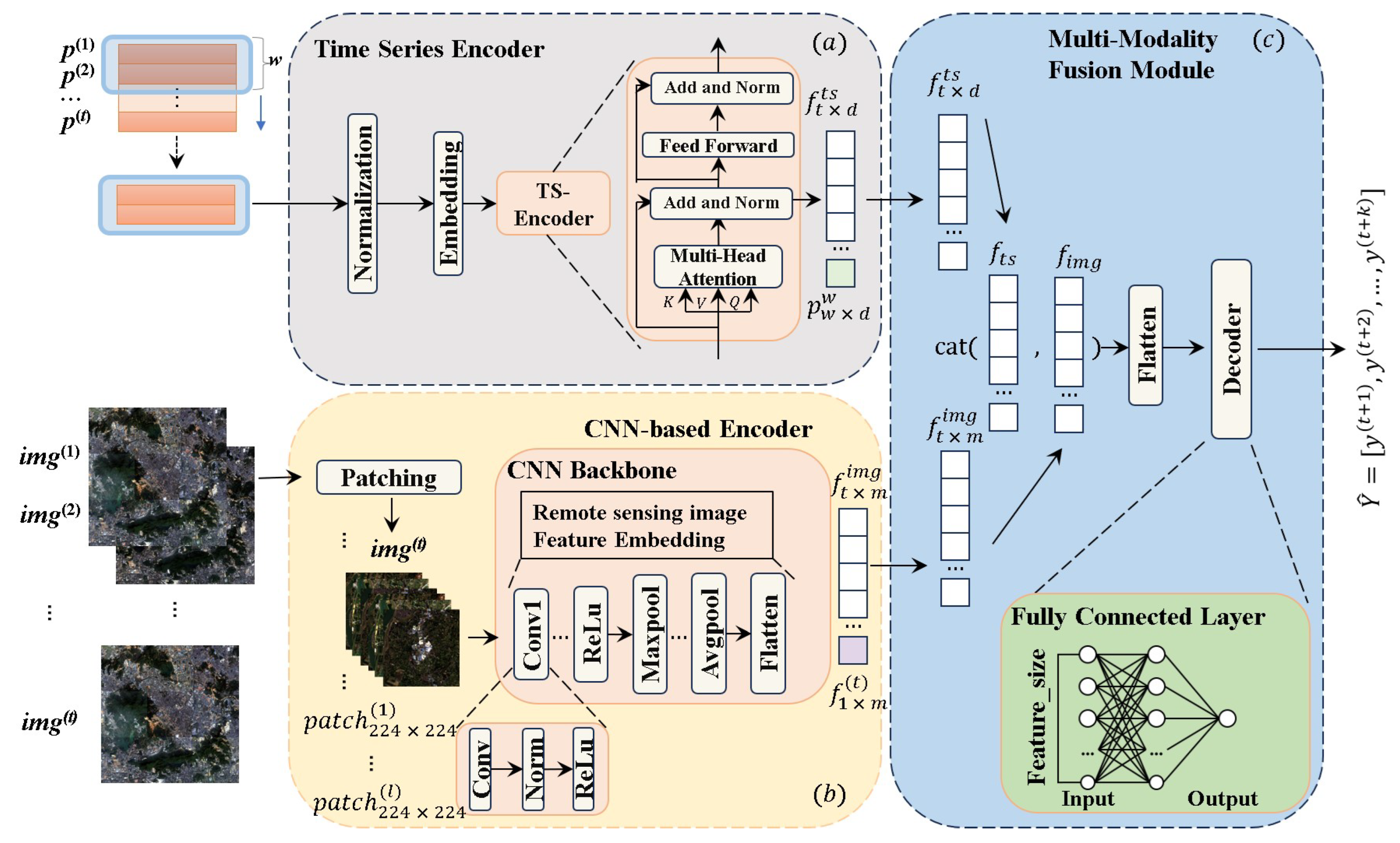
This study introduces remote sensing images into carbon price prediction and then proposes a Multi-source Fusion Time Series Transformer (MFTSformer) prediction model. To utilize useful information from remote sensing images, an encoder–decoder paradigm based on a powerful transformer is proposed to fuse the image and historical price data. In order to overcome the limitations of traditional recurrent-based neural networks with regards to long-term prediction, we utilize a multi-head self-attention mechanism from transformer models to model the input temporal data. We conduct various experiments on the carbon trading markets of a major city in China to validate the proposed strategy and methods. Our proposed MFTSformer method reduces errors by up to 52.24%, 45.07%, 18.42%, and 19.94% in comparison with the four baseline models. The results demonstrate that additional remote information is useful for accurately forecasting long-term urban carbon prices and that the MFTSformer method is effective.
The main contributions of this study are as follows:
  • We propose a multi-modal fusion carbon price prediction method called MFTSformer, which accurately predicts long-term urban carbon prices. Extensive experiments demonstrate that the proposed MFTSformer is capable of capturing the characteristics of long-term carbon price series and uncovering relevant information from remote sensing images. It can also support governments to formulate carbon pricing policies and companies to mitigate risks in practice.
  • Introducing urban remote sensing into carbon price forecasting helps us to capture the influential information of carbon price. As remote sensing imaging is objective, low-cost, and comprehensive, the results offer new insights for carbon researchers. In particular, as most carbon allowances come from forests, our work also provides information to researchers interested in forest carbon sequestration.
  • To the best of our knowledge, we are the first to introduce SOTA AI knowledge, such as an encoder–decoder framework, a self-attention mechanism, and multi-modal fusion technologies, to uncover remote sensing information for carbon price forecasting.

2. Literature Review

This section discusses the relationship between carbon pricing and forest carbon sequestration capacity, carbon price forecasting models, multi-source data fusion, and applications of urban remote sensing imagery, and it focuses on the importance of carbon price forecasting in forest science.

2.1. Carbon Price Impact on Forest Carbon Sequestration

There is a tight link between carbon prices and forest carbon sequestration capacity. The carbon price serves as an effective economic incentive mechanism that acts as a regulatory tool, urging companies to reduce carbon emissions [9]. In the carbon market, high-emission companies have to acquire enough carbon emission allowances to counterbalance their carbon emissions [4]. Forest carbon sequestration products are the carbon emission allowances in the carbon market [5,8]. This indicates that forest carbon sequestration projects tend to attract more investments as carbon prices rise, which, in turn, enhances their carbon sequestration capacity [11]. For example, Austin et al. [12] indicates that a carbon price set at appropriate levels can offer economic incentives for forest management to improve forest carbon sequestration. Moreover, improving forest management can increase forest carbon sequestration [42]. However, the influence of different types of forest management on carbon sequestration is complex, and the regulatory role of carbon prices can assist in selecting management strategies. When carbon prices reach a certain level, part of the economic and ecological value of forests match, motivating governments to prioritize forest carbon sequestration and conservation. In summary, carbon prices serve as a guide for forest managers [13]. Due to the volatility and uncertainty of carbon prices, managers need to consider potential market risks. Predicting carbon price changes accurately can provide indicators for managers to formulate robust forest carbon sequestration strategies in an uncertain carbon price environment. In summary, forest carbon trading mechanisms in carbon markets can foster forest carbon sequestration and aid carbon neutrality, as evidenced by numerous studies [11,12,13,42]. Accurate carbon price prediction, therefore, has caused extensive concerns in forest science [8,11,12,13].

2.2. Carbon Price Prediction Method

There are statistical and AI methods employed in the forecast of carbon prices; while statistical time prediction models, such as GARCH and ARIMA, have difficulties modeling the nonlinear characteristics of time series and are unable to effectively handle carbon price sequences, AI methods have been employed with more success [17]. AI models that predict carbon prices can be divided into two categories: traditional machine learning models and emerging deep learning models [14]. The application of extensive machine learning models has proven to be nonlinearly advantageous in predicting carbon prices [19,20,43]. For example, Jianwei et al. [19] utilized an LSSVR model to forecast carbon prices, resolving the issue of nonlinearity inherent in carbon price sequences. Zhang et al. [20] collaborated on the Complete Ensemble Empirical Mode Decomposition with Adaptive Noise (CEEMDAN) methodology with the XGBoost method to predict nonlinearity carbon prices. The CEEMDAN method was used to decompose the initial carbon price data into multiple subsequences, which were processed and used as input to the XGBoost model, providing good robustness performance. Zhang et al. [43] proposed an Extreme Learning Machine (ELM) optimized by a cosine-based whale optimization algorithm. However, these machine learning models struggle to generate accurate carbon price predictions over extended time frames due to inadequate processing of time-series data.
To improve price prediction accuracy, stronger nonlinear modeling capabilities using deep learning have been introduced [36,38,44]. For example, Nadirgil [44] used a GRU model to forecast carbon prices. The experimental results showed that their model significantly outperformed traditional machine learning models. Zhang and Wen [36] proposed an improved deep neural network model (TCN-Seq2Seq) to predict carbon prices, utilizing a sequence-to-sequence layout and full convolutional layers to learn temporal data dependencies. Huang et al. [38] established a novel decomposition–integration model, called VMD-GARCH/LSTM-LSTM, to predict carbon prices. These deep learning models have demonstrated greater adaptability to forecasting carbon prices but performed inadequately in long-term prediction [39,45]. In short, recurrent-based neural networks, such as LSTM, have insufficient capacity for long sequences [46]. Fortunately, transformer models perform better than recurrent-based networks in capturing long-term dependencies [40]. Given that carbon prices are influenced by many factors, similar to stock prices, it is challenging to use transformer models for producing long-term carbon price forecasts.

2.3. Multi-Source Data and Remote Sensing Image

The inclusion of data from multiple sources has been shown to improve the accuracy of carbon price predictions [28], and most current research focuses on the fusion of textual and carbon price data [24,25]. For instance, Zhang and Xia [24] proposed a novel data-driven approach for carbon price prediction, which utilizes online news data and Google Trends. They applied word embedding algorithms to identify text features in online carbon market news and incorporated them into carbon price prediction using LSTM. Through comparative experiments, they demonstrated the effectiveness of text information in improving prediction accuracy. Pan et al. [25] mined keywords that investors are concerned about in online news texts and combined them with the LSTM model for carbon price prediction. The experimental results also indicated that the application of multi-source data can enhance the accuracy of carbon price prediction. However, due to the subjectivity and ambiguity of textual data, the processes of interpretation and analysis can be highly uncertain [27]. Instead, urban remote sensing includes a variety of information reflecting changes in cities and surrounding forested areas that can objectively and accurately reflect changes in urban development and the growth of vegetation [28,31,32]. By analyzing remote sensing images, the model should enhance carbon price predictions. Motivated by this, in this study, we propose a method for the application of fusing urban remote sensing images. Moreover, through our extensive investigation, we find that the transformer model has not yet been applied to multi-source data carbon price prediction. At the same time, it is also shown that deep learning SOTA models, which have played an important role in many fields, such as industry and economics, have not been sufficiently used in research on forestry disciplines. This study is also the first to use deep learning foundation models, such as transformer and CNN, for carbon price prediction based on remotely sensed multi-source data.
To this end, in this section, we clarify the relationship between forest carbon sequestration and carbon prices, discussing the suitability of urban remote sensing images in carbon price prediction and the motivations of this study. The proposed carbon price prediction method in this work, which integrates historical prices with remote sensing image data, can offer crucial guidance for both businesses and governments in practice. Moreover, with an extensive literature search, this study can serve as a bridge between carbon pricing and the field of forest carbon sequestration, offering new insights to forest science fields regarding powerful AI methods.

3. Materials and Methods

3.1. Dataset

The carbon price trading data used in this study were obtained from carbon emissions trading exchanges in China. However, the data and the proportion of carbon trading vary among different exchanges. It is noteworthy that the Guangzhou carbon emissions trading accounts for 32.14% of the national market [47], making it a representative indicator of the overall carbon trading market in the country. Another reason for our focus on Guangzhou is that it is the capital of Guangdong, the leading province in China in terms of total GDP over the past 30 years, and also a major industrial city in China, the demand for forest carbon products of which is very high. Naturally, Guangzhou is representative of the carbon pricing issues we are investigating in this city. In addition, data from the Guangzhou price market for the past eight years are open and easily accessible. Therefore, our study selects the carbon price time-series data from the Guangzhou carbon emissions trading exchange as the experimental data. The data from Guangzhou carbon emissions trading exchange (www.cnemission.com, accessed on 5 May 2023) were collected using web scraping techniques, covering the time span from January 2016 to February 2023. The dataset includes various features, such as trading dates, opening prices, highest and lowest prices, and closing prices. The data statistics information and examples of raw price data can be found in Table 1 and Table 2.
For the important part of the remote sensing image data, we use 16-bit data with bands 2–5, which have a pixel resolution of 30 m. The remote sensing data were obtained from a Landsat 8 Operational Land Imager (OLI) sensor [48]. The raw data were obtained from the official website of the United States Geological Survey (www.usgs.gov, accessed on 5 May 2023). Specifically, we selected unlabeled remote sensing image data of Guangzhou city from the website, covering the time period from 2016 to 2023. Examples of remote sensing images are shown in Table 3. In detail, the RGB remote sensing images were used for feature extraction, while the false color remote sensing images were used in the case study for intuitive visualization.

3.2. MFTSformer

The overall architecture of the proposed MFTSformer, based on CNN and transformer, is shown in Figure 1. As illustrated in Figure 1, MFTSformer is an encoder–decoder framework that includes a transformer-based time-series encoder, a CNN-based remote sensing image encoder, and a multi-modality decoder for handling features from multiple sources. The CNN-based remote sensing image encoder is used to extract feature vectors from images, while the time-series encoder extracts long-term temporal features. The multi-modality module combines the features through concatenation and decoder functions. In general, the model takes remote sensing images and time-series data as inputs, generates fused embedding features, and then feeds the fused features into the multi-modality decoder. Finally, the output is mapped to the target variable through a fully connected layer to obtain prediction results. Given input X = { ( p ( 1 ) , p ( 2 ) , , p ( t ) ) , ( i m g ( 1 ) , i m g ( 2 ) , , i m g ( t ) ) } , where p ( t ) R 1 × d and i m g ( t ) R h × w represent price and image data, respectively, at time t. The three main modules (i.e., time-series encoder, CNN-based encoder, and multi-modality fusion module, as shown in Figure 1) of the proposed model can be illustrated briefly with the following Equations (1)–(3), respectively:
f t × d t s = [ p w × d ( w ) , p w × d ( w ) , , p w × d ( w ) ] = T i m e _ E n c o d e r ( [ p ( 1 ) , p ( 2 ) , , p ( t ) ] ) ,
where f t × d t s represents the outputs of the time-series encoder, and p w × d ( w ) is the embedding features with a w sliding window.
f t × m i m g = [ f 1 × m ( 1 ) , f 1 × m ( 2 ) , , f 1 × m ( t ) ] = C N N _ E n c o d e r ( [ i m g ( 1 ) , i m g ( 2 ) , , i m g ( t ) ] ) ,
where f 1 × m ( t ) stands for the features embedded through a CNN-based visual encoder at time t, and m is the embedding dimension according to the visual encoder.
Y ^ 1 × k = Γ ( ( f t × d t s , f t × m i m g ) ) ,
where Y ^ 1 × k represents the predicted k-long-term carbon price, Γ ( ) is a decoder function, and ( ) is the feature fusion module that concatenates multi-source features on the time (i.e., t) dimension.

3.2.1. Time-Series Encoder

With regard to the time-series encoder, this study adopts a transformer to extract features from the time-series data. A transformer is a neural network architecture that does not rely on recurrent structures. It utilizes a self-attention mechanism to model sequences, allowing it to effectively capture long-term dependencies within sequences [49]. First, we standardize and normalize the time-series data. On the one hand, by encoding the positions on different levels of time granularity (i.e., year, month, and day), the model captures the temporal relationships and dependencies more effectively. For each time granularity variable t i in p, we normalize them by employing sine and cosine functions, as shown in Equation (4):
P o s = s i n ( 2 π t i T n u m ) , P o s = c o s ( 2 π t i T n u m ) ,
where t i represents the year, month, or day of the temporal data in the raw data, p. T n u m represents the predetermined coverage of the dataset in terms of years, the number of months in a year, or the number of days in a month. The positional encoding formula primarily utilizes the sine and cosine functions to process the temporal dates.
On the other hand, in order to prioritize the main target of interest, which is the carbon price, this study performs normalization on the carbon price. The normalization module reduces the distribution differences among each input time series, resulting in a more stable distribution of the model’s input [50]. Moreover, incorporating the sinusoidal positional encoding formula helps the model capture the positional relationships between different sequences.
In addition to the structure of the transformer time-series encoder, it consists of three encoder layers, each consisting of a multi-head self-attention layer and a feed-forward neural network layer. Particularly, the multi-head self-attention layer is the core component of the transformer and is defined in Equation (5):
A t t e n t i o n ( p w × d ( w ) , p w × d ( w ) , p w × d ( w ) ) = S o f t m a x ( p w × d ( w ) p w × d ( w ) T d ) p w × d ( w ) .
After the embedding and self-attention calculation of the model inputs, it goes through the fully connected feed-forward network layer. The fully connected feed-forward network layer consists of two fully connected layers and a ReLU activation function. One fully connected layer maps the input vector to an intermediate vector, and the second fully connected layer maps the intermediate vector back to the output vector.

3.2.2. CNN-Based Encoder

CNN is a type of neural network specifically designed for image processing, capable of extracting features from images through operations such as convolution and pooling [51]. In this study, a pretrained CNN model, ResNet18 [52], is utilized to extract features from remote sensing images. For each time, t, the remote sensing image, i m g ( t ) , is first patched to 224 × 224 size; then, these patches at the same time, t, are fed to the backbone network (RestNet 18 in this work) to obtain the extracted feature, f 1 × m ( t ) . The details are shown in Equation (6):
f 1 × m ( t ) = 1 c l = 1 z Φ r e s n e t ( c ) ( p a t c h 224 × 224 ( l ) ) ,
where Φ ( ) is the convolution layer function, z is the total number of patches at time, t, decided by the size of i m g t . c is the number of layers in ResNet18. Lastly, the extracted features are concatenated to the t × m dimension features according to Equation (2).

3.2.3. Multi-Modality Fusion Module

To integrate the information from the time series and remote sensing images, this study employs separate feature extraction methods for the two types of data. As a result, the carbon price feature, f t s , obtained by the transformer and the remote sensing image feature, f i m g , extracted from ResNet18 are fused in this multi-modality fusion module. For the sake of simplicity, we have spliced and fused these two features in the time dimension, t, using Equation (3). As the fully connected decoder is faster and accurate [53], the concatenation features are then mapped to the target variable through a fully connected layer for prediction. In particular, the quantity of output nodes in the completely connected layer is represented by k. That is, k denotes the length of the intended forecasted time series for the price of carbon. With this straightforward outcome and design, training and implementing the MFTsformer can be effortless and efficient.

4. Experimental Setup

In this section, we primarily discuss the data processing approach and provide an introduction to the experimental setup. Comparative experiments with baseline models and ablation experiments were carried out to demonstrate the effectiveness and superiority of the proposed method, as well as the benefits of incorporating remote sensing image information. Particularly, we conducted parameter experiments in the ablation study to determine the optimal parameter choices. Furthermore, we examined the efficacy of integrating urban remote sensing image data in carbon price prediction through both quantitative and qualitative approaches within a case study.

4.1. Data Preprocessing

In a carbon price prediction model, data preprocessing is a crucial step that directly affects the performance of the model and the accuracy of the prediction results. Figure 2 shows a schematic diagram of data preprocessing and depicts a preprocessing flow. As shown in Figure 2, the dataset used in this study consists of two parts: urban carbon price time-series data and remote sensing image. As there are a small number of missing daily carbon prices due to a small number of non-trading days, the urban carbon price time-series data and remote sensing image are not aligned in terms of temporal scale. To address the alignment issue, we employed linear interpolation, which involves using a straight line between two known data points to approximate the unknown data between them [54]. Due to the characteristics of city development, there was not much variation within a short time period since changes in urban construction and vegetation require a longer time to manifest [55]. Hence, only historical carbon price data were used for interpolation. Moreover, the number of missing data was small. Linear interpolation could benefit from less complexity than specifically designing a module that handles missing values. In particular, the linear interpolation used in this work is shown in Equation (7):
y i = y + y y x x ( x i x ) ,
where the range of i is related to the interpolation range; x and y represent the known dates and corresponding carbon prices, respectively; x and y represent the dates and carbon prices that are already known, respectively; x i represents the dates that need to be interpolated; and y i represents the predicted carbon prices for the interpolated dates.
On the other hand, the remote sensing image was first patched to the small images on different regions with 224 × 224 sizes at each time, t, according to Equation (6), as using small images reduced the burden on the model. Then, this study employed a CNN-based encoder technique to extract image features representing the overall region from multiple small images.

4.2. Evaluation Setup

In order to validate the effectiveness of the proposed model in this study, we divided the time-series data into two parts: the training set and the test set. During the experimental process, the training set was used for model training and optimization, and the test set was used for final performance evaluation and comparison with other models [56]. Because of the strong relationship between the data at moments before and after in a time series, a chronological approach to dividing the training data has been adopted by recent papers in mainstream time-series research [18,19,20,21]. For example, in addition to the field of carbon pricing research, chronologically training models in stock price forecasting helps models learn temporal dependence. Conversely, if the dataset is split randomly, this can lead to data leakage problems [57] in time-series data. Meanwhile, to avoid data leakage, the test data must come after the training data, which drastically reduces the data available for training and lowers the model performance if random division cannot guarantee the temporal relationship. Therefore, this study adopted a chronological approach to divide the datasets. It is important to note that the fusion of multi-source data in this study does not require any specific processing of the image data during data partitioning. In detail, the partitioning of the training set and test set is shown in Table 4.

4.3. Urban Carbon Price Forecasting

As mentioned in Section 1 and Section 2, statistical models, machine learning models, and recurrent-based deep neural networks are currently popular models used to forecast carbon prices. We selected three popular approaches from each of these three model categories to use as a baseline, i.e., RIMA, SVR, and LSTM models. At the same time, MFTSformer is based on transformer, so the transformer is also regarded as a baseline model. Hence, we carried out experiments on the proposed model and four baseline models using the same temporal dataset. Because only MFTSformer fuses historical urban carbon prices and remote sensing images, it is natural to validate the effectiveness of our approach (e.g., SOTA AI models are powerful in predicting carbon price, and urban remote sensing data contain a wealth of factors affecting carbon prices).
We used the Adaptive Moment Estimation (Adam) optimizer for parameter optimization and the Mean Squared Error (MSE) loss function, 1 n i = 1 n ( y y ^ ) 2 . To strictly validate the prediction model, different metrics, such as Mean Absolute Percentage Error (MAPE), Mean Absolute Error (MAE), and Root Mean Squared Error (RMSE), are used in the unseen test datasets [58]. Lower values of these metrics indicate better performance. The hyperparameters of the baseline models and the evaluation metric formulae for each model are shown in Table 5 and Table 6. Furthermore, the long-term performance and computational cost are compared.

4.4. Ablation Studies

This study utilized ablation experiments to understand the impact of the different parts of the proposed model and also explored the impact of data splitting approaches on the experimental results. To validate the effectiveness of the remote sensing image encoder, the temporal feature encoder and the multimodal decoder were kept fixed, and the Visual Geometry Group Network (VGG) [59] image feature extraction network was used to extract features from remote sensing images. The performance of the model was compared under different networks. Similarly, in the ablation experiment for the image encoder, the image feature extraction network and the decoder remain unchanged, and an LSTM temporal feature extraction network was used to extract features from temporal data. The performance of the model was compared under different networks. In addition, we conducted parameter experiments based on the two sets of ablation experiments. We modified the hyperparameters, such as optimization algorithms, training epochs, and learning rates, and performed experiments accordingly.

4.5. Case Study

4.5.1. Study of Remote Sensing Image

The changing trends observed in urban remote sensing images reflect the transitions in urban industrialization and the surrounding forest areas. By utilizing an image model to capture these changes and incorporating the variations in image features into carbon price prediction, the accuracy of carbon price forecasting can be significantly improved. Through showcasing the changes in urban remote sensing images and comparing them with the model’s predicted changes, we can visually and intuitively demonstrate the helpfulness of urban remote sensing image information in the prediction process.

4.5.2. Study of Urban Statistics

Unlike a visual presentation of remote sensing images, a fluctuation in carbon prices is strongly related to various industries within the city. To validate the consistency between the changes in urban remote sensing images and statistical metrics, we collected relevant statistical data. Furthermore, we compared the variations in statistical metrics with the predicted changes in carbon prices. This quantitative analysis provides further evidence of the effectiveness of urban remote sensing image information from a data-driven perspective.

5. Results and Discussion

5.1. Carbon Price Prediction Analysis

We conducted experiments on the proposed model and four other baseline models using the same temporal dataset. Table 7 presents the evaluation metric results for each model. These results are the averages obtained from three experiments. A relative error heatmap of the experimental models, calculated based on Table 7, is shown in Figure 3, which clearly and intuitively illustrates the differences between each model. In Figure 3, a matrix diagram shows the difference between the row and column models. In the lower-left column, looking from top to bottom, it can be seen that the other models improve relative to the row model at the starting point; in the upper-right column, looking from bottom to top, it can be seen that the row model relative to the starting column model exhibits an increase in the error ratio. Color depth represents the numerical value. A positive number means that the error has decreased, and a negative number means that the error has increased.
As shown in Table 7 and Figure 3, the advanced transformer model has a minimum MAE, MAPE, and RMSE of 0.586, 0.783%, and 0.686, respectively. It outperforms the other three baseline models in all windows by up to 48.50%, 44.58%, and 37.06%, respectively. These results suggest that the powerful SOTA AI methods are effective in predicting carbon prices. As indicated in Table 7, it is evident that our proposed MFTSformer approach outperforms all baseline models, including transformer, across all evaluation metrics and prediction window lengths. It is worth noting that MFTSformer outperforms ARIMA, SVR, and LSTM by up to 52.24%, 45.07%, and 18.42%, respectively. When compared to the original transformer, MFTSformer achieved a 14.6% reduction in MAE, a 10.38% decrease in RMSE, and a 19.94% decrease in MAPE. As MFTSformer provides additional information for remote areas compared to transformer, the evidence indicates that the enhancement is mostly due to the integration of urban remote sensing image features into MFTSformer.
Additionally, the MFTSformer model obtains optimum performance with longer-term prediction windows, as shown in Table 7. Specifically, with a prediction window of 64, MFTSformer exhibits average improvements of 39.84%, 36.31%, and 39.34% for MAE, MAPE, and RMSE, respectively. When the prediction window is 104, the MFTSformer demonstrates an average improvement of 38.94%, 32.32%, and 23% for MAE, MAPE, and RMSE, respectively. To further demonstrate the long-term prediction effect, the comparison results for each advanced AI model (i.e., LSTM, transformer, and MFTSformer) are illustrated in Figure 4. Compared to recurrent-based neural networks (i.e., LSTM), the accuracy of MFTSformer and transformer surpasses that of LSTM when dealing with long-term prediction windows. This is primarily attributed to the multi-head self-attention mechanism in the transformer framework, which enables the capturing of long-term dependencies in time-series data. Particularly, MFTSformer has a lower prediction error than transformer and successfully predicts the trend of carbon prices for the next 104 days, as shown in Figure 4. Conversely, LSTM performed poorly. We suspect that this is due to gradient vanishing issues in long time-series prediction. These experimental results emphasize the superiority of MFTSformer in long-term prediction.
Figure 5 shows the performance with different training epochs. Figure 6 depicts the declining loss trend at each stage of the MFTSformer model training process over 100 epochs. As shown in Figure 5 and Figure 6, MFTSformer could perform well with only 10 epochs, and the training loss converges rapidly. These results suggest that our proposed method requires fewer training resources and that MFTSformer can quickly adapt to a rapidly changing carbon market with retraining. Therefore, MFTSformer is expected to perform well in practice.
Moreover, we compared the advantages and disadvantages of two popular time-series processing approaches, namely, transformer and LSTM, from a temporal perspective. We first conducted a theoretical analysis of the time complexity for LSTM and transformer. LSTM is a kind of recurrent neural network that performs computations at each time step. Within a single time step, the main calculations involve gate computations, matrix multiplications, new state calculations, and updated hidden state calculations. Assuming the dimension of the hidden state is d, the computational complexity within a time step is approximately O ( d 2 ) . With t as the sequence length, the overall time complexity of LSTM is roughly O ( t · d 2 ) . On the contrary, the self-attention mechanisms of transformer enable a certain level of parallel computation. For a feature vector with d as its dimension, self-attention computation’s time complexity at one position is O ( d 2 ) . If there are h attention heads and the sequence length is t, the overall time complexity of self-attention becomes O ( h · t · d 2 ) . The transformer also includes computations for feed-forward neural networks with a time complexity of O ( t · d · d f f ) , where d f f is the intermediate layer dimension of the feed-forward network. Thus, the overall time of transformer complexity is O ( h · t · d 2 + t · d · d f f ) . Theoretically, looking at a single time step, LSTM has a lower time complexity compared to transformer, making its calculations simpler. However, when considering sequence length, the transformer benefits from parallel computation, whereas LSTM computes sequentially. This means that for long sequences, transformer can be faster due to its parallel processing capability, making it useful in practice. Our computational experiments also support this observation. The calculation time of LSTM, transformer, and MFTSformer are shown in Table 8. In the case of the 104 prediction window, the training times for the LSTM and transformer are 24.47 s and 21.53 s, respectively. This is possibly due to the multi-head attention mechanism in the transformer, which involves computing attention weights and corresponding values. When the prediction windows are set to 64 and 104, transformer is approximately 11.54% and 12.01% faster, respectively, in terms of training time compared to LSTM. Although the computational time of MFTSformer is slightly longer than that of LSTM and transformer, the reason for this is the additional data preprocessing computations. However, this point is relatively insignificant, and the difference in the MFTS transformer will become negligible in real-world scenarios as the magnitude of data increases.
In short, compared to conventional models, MFTSformer presents comprehensive performance benefits. The advanced self-attention mechanism and additional urban remote sensing images can accurately predict carbon price. These findings support the two motivations of this study; that is, the SOTA AI model provides a powerful forecasting ability and the extra remote sensing reflecting urban human activities is useful. In addition, the low-cost training resources make the proposed MFTSformer method a potential tool for managing carbon price in practice.

5.2. Ablation Studies Analysis

In this section, we compared the different modules of the proposed model based on the perspective of the image feature encoder and the time-series feature encoder. Initially, we evaluated the significance of each module integrated into our proposed framework by comparing the prediction performance of the various modules under the same conditions. In an identical dataset, we substituted a ResNet component with a VGG image processing component and swapped the transformer encoder composition with an LSTM temporal feature extraction network. Through testing various model components, we can authenticate the efficacy of each component within the model and comprehend the influence of diverse components on the experimental results.
Table 9 shows the long-term prediction results for different combinations of image encoder and time-series encoder models (i.e., the window is 104). According to Table 9, MFTSformer demonstrates a maximum improvement of 18.40% in performance compared to ResNet-LSTM, while VGG-transformer exhibits a maximum improvement of 11.57% over VGG-LSTM. These results indicate that the transformer time-series encoder outperforms LSTM in terms of prediction performance. In addition, Table 9 reveals that MFTSformer enhances the performance of MFTSformer over VGG-transformer by up to 4.4%, while ResNet-LSTM improves the performance of ResNet-LSTM over VGG-LSTM by up to 1.6%. These results indicate that the ResNet image encoder outperforms VGG in long-term sequence prediction. In conclusion, our proposed MFTSformer method utilizes ResNet and transformer modules to improve long-term sequence prediction.
In addition, we conducted the ablation experiments regarding data split methods and dataset sizes using MFTSformer as the experimental model. Different data split methods were chosen to validate the impact of chronological order and random split on prediction outcomes. A small dataset from 2016 to 2021 including training and testing data, two years less than that data of the comparison experiments, was used to investigate the effect of data split ablation experiments. The experimental results are presented in Table 10. From Table 10, it can be observed that the prediction results using the chronological order data split method are superior to those achieved using random partitioning. This difference primarily stems from the fact that models learning from time-series data need to capture patterns and trends within different time periods. Training the model in a chronological order manner allows it to gradually adapt to changes at different time points, thereby enhancing its generalization to future time points. In terms of dataset size, reducing the volume of data, whether utilizing chronological or random splitting, will lead to a decline in performance. This is a consequence of the fact that the random partitioning method, which requires more data to achieve the same level of efficiency, is inferior. Hence, the proposed training approach in this study, utilizing chronological order training, is more appropriate as it aligns well with the temporal characteristics of data and aids the model in learning temporal dependencies.
In the hyperparameter ablation experiments, we explored the effects of gradient optimization algorithms and learning rates on the performance. In this study, we varied the optimization algorithm and learning rate, specifically selecting Adam and Stochastic Gradient Descent (SGD) as the algorithms and choosing learning rates of 0.001 and 0.0001. We performed four experiments and obtained different prediction results, as shown in Table 11. The experiments that utilized the Adam algorithm and a learning rate of 0.0001 exhibited the best predictive performance, which is in accordance with commonly held expectations. The average accuracy of this model improved by 4.6% and 4% compared to the models that used the SGD optimization algorithm with a learning rate of 0.001. The Adam algorithm is recognized for its speedy and effective optimization, rendering it better equipped for the scenario presented in this study. In contrast, the SGD algorithm usually necessitates longer training times, experiences slower convergence, and is more sensitive to the learning rate. Consequently, the SGD algorithm exhibited lackluster performance when the learning rate was set to 0.001. Based on the experimental results, it can be concluded that the Adam algorithm generally outperforms the SGD algorithm. Furthermore, the accuracy of the prediction results is heavily influenced by the learning rate. As the learning rate has a significant impact on the prediction results, it is necessary to perform real-time fine-tuning based on the optimization algorithm and model when adopting this method in practice. Therefore, in this study, a learning rate of 0.0001 and the Adam algorithm were selected.

5.3. Case Study Analysis

In order to prove the correctness of the intention to integrate urban remote sensing information more vividly and intuitively, this study adopts the form of a case study analysis. The case we chose is a remote sensing image of Guangzhou City, with changes from 2016 to 2021. The results indicate that the model’s use of image information to make predictions is evident.

5.3.1. Urban Statistics Changes

To illustrate the effectiveness of urban remote sensing image information in carbon price prediction, we conducted a statistical analysis on various data aspects of the experimental area. These factors include parameters such as green area, urbanization development, and the ratio of heavy industry to light industry. The statistical data are all from the official statistical yearbook of Guangzhou City. This analysis demonstrates that the changes observed in urban remote sensing images are both genuine and visually reflective of urban transformations. By incorporating these image-based insights, we were able to improve the accuracy of carbon price prediction from an image-oriented perspective.
The statistical analysis of urban data is displayed in Figure 7, Figure 8, Figure 9 and Figure 10. Figure 7 provides a line chart showing the annual changes in the gross domestic product (GDP) of the three major industries in Guangzhou. It is evident that this industry has a relatively small proportion, with a growth rate of 41.8% due to its small initial base. The secondary industry remains stable and experienced positive growth of 29.03% over the last five years, while the tertiary industry exhibits vigorous development with a remarkable 48% growth, driven by its substantial base. These three major industries have a significant impact on the urban environment and directly influence carbon prices. Figure 8 presents the proportion of the three major industries during key years, with the tertiary industry averaging a 70.8% share, highlighting its dominant influence. Figure 9 illustrates the green coverage values in Guangzhou between 2016 and 2021, revealing a decrease in the green coverage rate in the built-up areas during 2021. Consequently, carbon prices experienced significant fluctuation in 2021, with an increasing upward trend. Figure 10 visually presents the industry data and green coverage data of Guangzhou through a heatmap. The results indicate that the tertiary industry has undergone significant changes, while the green coverage data have remained relatively stable. Therefore, these results reflect that the remote sensing image is an indicator of the industrialization of previously unused land.

5.3.2. Analysis of the Integrated Urban Characteristics

Analyzing the changes in urban statistics, as mentioned in Section 5.3.1, it is evident that cities undergo significant transformations and their effect on the carbon price cannot be overlooked. Consequently, utilizing urban change data to predict carbon prices is plausible. The utilization of urban remote sensing image information can enhance the accuracy of carbon price prediction. Firstly, we visualize the changes in urban remote sensing images and correlate them with the corresponding years of urban development. Then, we compare the predicted carbon prices with the actual prices during the same time period to evaluate whether the information from urban remote sensing images indeed improves the prediction accuracy.
As shown in Figure 11, the proposed MFTSformer has captured the decrease in forest and green spaces around the city. The noticeable decline in urban greenery over time is consistent with our model’s accurate prediction of price fluctuations within this range. Furthermore, MFTSformer accurately predicts price changes within this range, supporting the premise that image data from urban remote sensing improves prediction accuracy.
In particular, as illustrated in Figure 11, it can be observed that the green vegetation coverage in urban remote sensing images decreased from 2016 to 2017, indicating further urban industrialization. The fluctuation in carbon prices is linked to these factors. As illustrated in Figure 11a, the carbon price trend is on an upward trajectory and our model accurately predicts this trend. The upward trend continues between 2017 and 2019. From 2019 to 2021, rapid urban development caused an acceleration in carbon price changes. Nevertheless, the model remains capable of accurately reflecting changing trends and limiting errors within a specific range. Upon contrasting predicted values with and without image data, it can be inferred that incorporating image information aids carbon price prediction. This indicates the model’s sensitivity to urban remote sensing images and the efficacy of using image data in prediction.

6. Conclusions

This study introduced an SOTA self-attention and encoder–decoder paradigm to explore the influence of remote sensing information on urban carbon prices. We proposed the MFTSformer method for long-term urban carbon price prediction by fusing remote sensing images and historical urban price data. All comparison experiments, ablation experiments, and case studies demonstrated the effectiveness of MFTSformer. Our research findings suggest that urban remote sensing images can reflect human economic activities that have a direct impact on urban carbon prices. Due to the high accuracy and relatively low training requirements for forecasting long-term carbon prices, they can be useful for government and companies. Additionally, the advanced AI mechanism employed in this study can provide insights for future research in the field of forest science. However, certain limitations remain because some factors have not been taken into account, such as the effect of policy uncertainty and natural disasters [60]. Moreover, research on carbon neutrality in the realm of deep learning [61] indicates that there may be alternative methods for carbon price prediction. In future research, these factors will be further investigated based on the available information.

Author Contributions

Conceptualization, C.M., Z.X. and X.C.; methodology, C.M. and Z.X.; software, Z.X. and C.M.; validation, Z.X. and C.M.; formal analysis, C.M. and Z.X.; investigation, Z.X.; resources, C.M., Z.X. and X.C.; data curation, Z.X. and Y.L.; writing—original draft preparation, C.M. and Z.X.; writing—review and editing, C.M., X.C. and Z.X.; visualization, Z.X., Y.L., H.L. and S.Y.; supervision, C.M., Y.L. and X.C.; project administration, C.M. and X.C.; funding acquisition, C.M. and X.C.; significant contributions, C.M., Z.X. and X.C. All authors have read and agreed to the published version of the manuscript.

Funding

This research was funded by Ant Group through the CCF-Ant Research Fund (CCF-AFSG RF20220214) and Outstanding Youth Team Project of Central Universities (QNTD202308).

Data Availability Statement

Not applicable.

Acknowledgments

The authors are grateful to Liheng Zhong of the Ant Group for valuable discussions. The authors thank the anonymous reviewers for their valuable comments.

Conflicts of Interest

The authors declare no conflict of interest.

References

  1. Dong, H.; Xue, M.; Xiao, Y.; Liu, Y. Do carbon emissions impact the health of residents? Considering China’s industrialization and urbanization. Sci. Total Environ. 2021, 758, 143688. [Google Scholar] [CrossRef] [PubMed]
  2. Wang, X.; Yan, L. Measuring the integrated risk of China’s carbon financial market based on the copula model. Environ. Sci. Pollut. Res. 2022, 29, 54108–54121. [Google Scholar] [CrossRef] [PubMed]
  3. Yechen, F.; Xiaoping, Y. Research on the Fluctuation Characteristics of Carbon Allowance Price Based on ARMA-GARCH Cluster Model. China For. Econ. 2023, 2, 100–106. [Google Scholar]
  4. Shen, Y.; Gao, T.; Song, Z.; Ma, J. Closed-Loop Supply Chain Decision-Making and Coordination Considering Fairness Concerns under Carbon Neutral Rewards and Punishments. Sustainability 2023, 15, 6466. [Google Scholar] [CrossRef]
  5. Cao, X.L.; Li, X.S.; Breeze, T.D. Quantifying the carbon sequestration costs for Pinuselliottii afforestation project of China greenhouse gases voluntary emission reduction program: A case study in Jiangxi Province. Forests 2020, 11, 928. [Google Scholar] [CrossRef]
  6. Shi, P.; Chen, X. Supply chain decision-making and coordination for joint investment in cost and carbon emission reduction. Int. J. Low-Carbon Technol. 2023, 18, 306–321. [Google Scholar] [CrossRef]
  7. Cheng, S.; Huang, X.; Chen, Y.; Dong, H.; Li, J. Carbon Sink Performance Evaluation and Socioeconomic Effect of Urban Aggregated Green Infrastructure Based on Sentinel-2A Satellite. Forests 2022, 13, 1661. [Google Scholar] [CrossRef]
  8. Zeng, S.; Fu, Q.; Yang, D.; Tian, Y.; Yu, Y. The Influencing Factors of the Carbon Trading Price: A Case of China against a “Double Carbon” Background. Sustainability 2023, 15, 2203. [Google Scholar] [CrossRef]
  9. Chen, X.; Lin, B. Towards carbon neutrality by implementing carbon emissions trading scheme: Policy evaluation in China. Energy Policy 2021, 157, 112510. [Google Scholar] [CrossRef]
  10. Weng, Z.; Ma, Z.; Xie, Y.; Cheng, C. Effect of China’s carbon market on the promotion of green technological innovation. J. Clean. Prod. 2022, 373, 133820. [Google Scholar] [CrossRef]
  11. Ke, S.; Zhang, Z.; Wang, Y. China’s forest carbon sinks and mitigation potential from carbon sequestration trading perspective. Ecol. Indic. 2023, 148, 110054. [Google Scholar] [CrossRef]
  12. Austin, K.; Baker, J.; Sohngen, B.; Wade, C.; Daigneault, A.; Ohrel, S.; Ragnauth, S.; Bean, A. The economic costs of planting, preserving, and managing the world’s forests to mitigate climate change. Nat. Commun. 2020, 11, 5946. [Google Scholar] [CrossRef] [PubMed]
  13. Zhou, B.; Zhang, C.; Wang, Q.; Zhou, D. Does emission trading lead to carbon leakage in China? Direction and channel identifications. Renew. Sustain. Energy Rev. 2020, 132, 110090. [Google Scholar] [CrossRef]
  14. Deb, C.; Zhang, F.; Yang, J.; Lee, S.E.; Shah, K.W. A review on time series forecasting techniques for building energy consumption. Renew. Sustain. Energy Rev. 2017, 74, 902–924. [Google Scholar] [CrossRef]
  15. Byun, S.J.; Cho, H. Forecasting carbon futures volatility using GARCH models with energy volatilities. Energy Econ. 2013, 40, 207–221. [Google Scholar] [CrossRef]
  16. Zhu, B.; Chevallier, J.; Zhu, B.; Chevallier, J. Carbon price forecasting with a hybrid Arima and least squares support vector machines methodology. In Pricing and Forecasting Carbon Markets: Models and Empirical Analyses; Springer: Cham, Switzerland, 2017; pp. 87–107. [Google Scholar]
  17. Zhu, B.; Ye, S.; Wang, P.; He, K.; Zhang, T.; Wei, Y.M. A novel multiscale nonlinear ensemble leaning paradigm for carbon price forecasting. Energy Econ. 2018, 70, 143–157. [Google Scholar] [CrossRef]
  18. Zhu, B.; Han, D.; Wang, P.; Wu, Z.; Zhang, T.; Wei, Y.M. Forecasting carbon price using empirical mode decomposition and evolutionary least squares support vector regression. Appl. Energy 2017, 191, 521–530. [Google Scholar] [CrossRef]
  19. Jianwei, E.; Ye, J.; He, L.; Jin, H. A denoising carbon price forecasting method based on the integration of kernel independent component analysis and least squares support vector regression. Neurocomputing 2021, 434, 67–79. [Google Scholar]
  20. Zhang, C.; Zhao, Y.; Zhao, H. A novel hybrid price prediction model for multimodal carbon emission trading market based on CEEMDAN algorithm and window-based XGBoost approach. Mathematics 2022, 10, 4072. [Google Scholar] [CrossRef]
  21. Huang, Y.; He, Z. Carbon price forecasting with optimization prediction method based on unstructured combination. Sci. Total Environ. 2020, 725, 138350. [Google Scholar] [CrossRef]
  22. Hong, T.; Pinson, P.; Wang, Y.; Weron, R.; Yang, D.; Zareipour, H. Energy forecasting: A review and outlook. IEEE Open Access J. Power Energy 2020, 7, 376–388. [Google Scholar] [CrossRef]
  23. Lu, H.; Ma, X.; Ma, M.; Zhu, S. Energy price prediction using data-driven models: A decade review. Comput. Sci. Rev. 2021, 39, 100356. [Google Scholar] [CrossRef]
  24. Zhang, F.; Xia, Y. Carbon price prediction models based on online news information analytics. Finance Res. Lett. 2022, 46, 102809. [Google Scholar] [CrossRef]
  25. Pan, D.; Zhang, C.; Zhu, D.; Hu, S. Carbon price forecasting based on news text mining considering investor attention. Environ. Sci. Pollut. Res. 2023, 30, 28704–28717. [Google Scholar] [CrossRef]
  26. Wang, P.; Liu, J.; Tao, Z.; Chen, H. A novel carbon price combination forecasting approach based on multi-source information fusion and hybrid multi-scale decomposition. Eng. Appl. Artif. Intell. 2022, 114, 105172. [Google Scholar] [CrossRef]
  27. Bai, Y.; Li, X.; Yu, H.; Jia, S. Crude oil price forecasting incorporating news text. Int. J. Forecast. 2022, 38, 367–383. [Google Scholar] [CrossRef]
  28. Yang, J.; Yang, Y.; Wen, J.; Li, Y.; Ercisli, S. Remote sensing image information quality evaluation via node entropy for efficient classification. Remote Sens. 2022, 14, 4400. [Google Scholar] [CrossRef]
  29. Bherwani, H.; Banerji, T.; Menon, R. Role and value of urban forests in carbon sequestration: Review and assessment in Indian context. Environ. Dev. Sustain. 2022, 1–24. [Google Scholar] [CrossRef]
  30. Alpaidze, L.; Salukvadze, J. Green in the City: Estimating the Ecosystem Services Provided by Urban and Peri-Urban Forests of Tbilisi Municipality, Georgia. Forests 2023, 14, 121. [Google Scholar] [CrossRef]
  31. Song, J.; Gao, S.; Zhu, Y.; Ma, C. A survey of remote sensing image classification based on CNNs. Big Earth Data 2019, 3, 232–254. [Google Scholar] [CrossRef]
  32. Zhu, Z.; Zhou, Y.; Seto, K.C.; Stokes, E.C.; Deng, C.; Pickett, S.T.; Taubenböck, H. Understanding an urbanizing planet: Strategic directions for remote sensing. Remote Sens. Environ. 2019, 228, 164–182. [Google Scholar] [CrossRef]
  33. Kattenborn, T.; Leitloff, J.; Schiefer, F.; Hinz, S. Review on Convolutional Neural Networks (CNN) in vegetation remote sensing. ISPRS J. Photogramm. Remote Sens. 2021, 173, 24–49. [Google Scholar] [CrossRef]
  34. Astolfi, G.; Cesar Rezende, F.P.; De Andrade Porto, J.V.; Matsubara, E.T.; Pistori, H. Syntactic Pattern Recognition in Computer Vision: A Systematic Review. ACM Comput. Surv. 2022, 54, 1–35. [Google Scholar] [CrossRef]
  35. Li, H.; Huang, X.; Zhou, D.; Cao, A.; Su, M.; Wang, Y.; Guo, L. Forecasting carbon price in China: A multimodel comparison. Int. J. Environ. Res. Public Health 2022, 19, 6217. [Google Scholar] [CrossRef] [PubMed]
  36. Zhang, F.; Wen, N. Carbon price forecasting: A novel deep learning approach. Environ. Sci. Pollut. Res. 2022, 29, 54782–54795. [Google Scholar] [CrossRef]
  37. Liu, H.; Shen, L. Forecasting carbon price using empirical wavelet transform and gated recurrent unit neural network. Carbon Manag. 2020, 11, 25–37. [Google Scholar] [CrossRef]
  38. Huang, Y.; Dai, X.; Wang, Q.; Zhou, D. A hybrid model for carbon price forecasting using GARCH and long short-term memory network. Appl. Energy 2021, 285, 116485. [Google Scholar] [CrossRef]
  39. Glorot, X.; Bengio, Y. Understanding the difficulty of training deep feedforward neural networks. In Proceedings of the Thirteenth International Conference on Artificial Intelligence and Statistics, Sardinia, Italy, 13–15 May 2010; pp. 249–256. [Google Scholar]
  40. Vaswani, A.; Shazeer, N.; Parmar, N.; Uszkoreit, J.; Jones, L.; Gomez, A.N.; Kaiser, Ł.; Polosukhin, I. Attention is all you need. Adv. Neural Inf. Process. Syst. 2017, 30, 5998–6008. [Google Scholar]
  41. OpenAI. GPT-4 Technical Report. arXiv 2023, arXiv:2303.08774. [Google Scholar]
  42. Daigneault, A.; Baker, J.S.; Guo, J.; Lauri, P.; Favero, A.; Forsell, N.; Johnston, C.; Ohrel, S.B.; Sohngen, B. How the future of the global forest sink depends on timber demand, forest management, and carbon policies. Glob. Environ. Change 2022, 76, 102582. [Google Scholar] [CrossRef]
  43. Zhang, W.; Wu, Z.; Zeng, X.; Zhu, C. An ensemble dynamic self-learning model for multiscale carbon price forecasting. Energy 2023, 263, 125820. [Google Scholar] [CrossRef]
  44. Nadirgil, O. Carbon price prediction using multiple hybrid machine learning models optimized by genetic algorithm. J. Environ. Manag. 2023, 342, 118061. [Google Scholar] [CrossRef] [PubMed]
  45. Zhang, F.; Tian, X.; Zhang, H.; Jiang, M. Estimation of aboveground carbon density of forests using deep learning and multisource remote sensing. Remote Sens. 2022, 14, 3022. [Google Scholar] [CrossRef]
  46. Zhou, H.; Zhang, S.; Peng, J.; Zhang, S.; Li, J.; Xiong, H.; Zhang, W. Informer: Beyond efficient transformer for long sequence time-series forecasting. Proc. AAAI Conf. Artif. Intell. 2021, 35, 11106–11115. [Google Scholar] [CrossRef]
  47. Lo, A.Y.; Mai, L.Q.; Lee, A.K.Y.; Francesch-Huidobro, M.; Pei, Q.; Cong, R.; Chen, K. Towards network governance? The case of emission trading in Guangdong, China. Land Use Policy 2018, 75, 538–548. [Google Scholar] [CrossRef]
  48. Vermote, E.; Justice, C.; Claverie, M.; Franch, B. Preliminary analysis of the performance of the Landsat 8/OLI land surface reflectance product. Remote Sens. Environ. 2016, 185, 46–56. [Google Scholar] [CrossRef]
  49. Jiang, K.; Peng, P.; Lian, Y.; Xu, W. The encoding method of position embeddings in vision transformer. J. Vis. Commun. Image Represent. 2022, 89, 103664. [Google Scholar] [CrossRef]
  50. Passalis, N.; Tefas, A.; Kanniainen, J.; Gabbouj, M.; Iosifidis, A. Deep adaptive input normalization for time series forecasting. IEEE Trans. Neural Netw. Learn. Syst. 2019, 31, 3760–3765. [Google Scholar] [CrossRef]
  51. LeCun, Y.; Bottou, L.; Bengio, Y.; Haffner, P. Gradient-based learning applied to document recognition. Proc. IEEE 1998, 86, 2278–2324. [Google Scholar] [CrossRef]
  52. He, K.; Zhang, X.; Ren, S.; Sun, J. Deep residual learning for image recognition. In Proceedings of the IEEE Conference on Computer Vision and Pattern Recognition, Las Vegas, NV, USA, 27–30 June 2016; pp. 770–778. [Google Scholar]
  53. Zeng, A.; Chen, M.; Zhang, L.; Xu, Q. Are transformers effective for time series forecasting? Proc. AAAI Conf. Artif. Intell. 2023, 37, 11121–11128. [Google Scholar] [CrossRef]
  54. Raubitzek, S.; Neubauer, T. A fractal interpolation approach to improve neural network predictions for difficult time series data. Expert Syst. Appl. 2021, 169, 114474. [Google Scholar] [CrossRef]
  55. Xue, J.; Su, B. Significant remote sensing vegetation indices: A review of developments and applications. J. Sens. 2017, 2017, 1353691. [Google Scholar] [CrossRef]
  56. Hao, Y.; Tian, C.; Wu, C. Modelling of carbon price in two real carbon trading markets. J. Clean. Prod. 2020, 244, 118556. [Google Scholar] [CrossRef]
  57. Papadimitriou, P.; Garcia-Molina, H. Data leakage detection. IEEE Trans. Knowl. Data Eng. 2010, 23, 51–63. [Google Scholar] [CrossRef]
  58. Segnon, M.; Lux, T.; Gupta, R. Modeling and forecasting the volatility of carbon dioxide emission allowance prices: A review and comparison of modern volatility models. Renew. Sustain. Energy Rev. 2017, 69, 692–704. [Google Scholar] [CrossRef]
  59. Simonyan, K.; Zisserman, A. Very deep convolutional networks for large-scale image recognition. arXiv 2014, arXiv:1409.1556. [Google Scholar]
  60. Sun, L.L.; Cui, H.J.; Ge, Q.S. Will China achieve its 2060 carbon neutral commitment from the provincial perspective? Adv. Clim. Chang. Res. 2022, 13, 169–178. [Google Scholar] [CrossRef]
  61. Mou, C.; Wei, M.; Liu, H.; Chen, Z.; Cui, X. A Spatio-Temporal Neural Network Learning System for City-Scale Carbon Storage Capacity Estimating. IEEE Access 2023, 11, 31304–31322. [Google Scholar]
Figure 1. A structural diagram of MFTSformer: (a) The time-series feature extractor of the model, where the temporal data are normalized before being input to the network structure and processed by an encoder to obtain a time-series feature vector with sliding windows; (b) The remote sensing image feature extractor of the model, where the image input undergoes a transformation and is processed by a convolutional neural network to obtain a feature vector; (c) The multimodal fusion module of the model fuses the embedding feature vectors. Finally, the fused vector is passed through the decoder, which is the fully connected layer, to obtain the final prediction result.
Forests 14 01989 g001
Figure 2. A schematic diagram of data preprocessing: (a) depicts the urban carbon price data preprocessing flow. The missing values in price time series are filled by using linear interpolation; (b) depicts the data processing flow of fusing the prices time series and remote images series. The arrows represent the data flow.
Forests 14 01989 g002
Figure 3. The heatmap of relative errors.
Forests 14 01989 g003
Figure 4. Carbon price prediction results. Visualization results of LSTM, transformer, and MFTSformer: (ac) Carbon price prediction results of LSTM, transformer, and MFTSformer, respectively, on the same time-series dataset. In the case of MFTSformer, additional urban remote sensing images are incorporated into the data.
Forests 14 01989 g004
Figure 5. The performance of MFTSformer with different training epochs: (ad) Performance of the model with 10, 30, 60, 100 training epochs, respectively.
Forests 14 01989 g005
Figure 6. Figure shows the trend of training loss.
Forests 14 01989 g006
Figure 7. The changes in output value of the three major industries in Guangzhou from 2016 to 2021.
Forests 14 01989 g007
Figure 8. The proportions of the three major industries at key years. The changes in output value of the three major industries in Guangzhou from 2016 to 2021.
Forests 14 01989 g008
Figure 9. The changes in the amount of landscape investment and the green coverage rate of the built-up areas in Guangzhou from 2016 to 2021. (a) Detailed investment amount. (b) Line chart depicting the changes in green coverage rate.
Forests 14 01989 g009
Figure 10. The heatmap of industries, green coverage, and years. The left image shows the heatmap of industries and years, while the right image shows the heatmap of green coverage and years. The changes in output value of the three major industries in Guangzhou from 2016 to 2021.
Forests 14 01989 g010
Figure 11. False color urban remote sensing images from 2016 to 2021 and prediction images of key points. It can be observed that the green vegetation coverage in the red areas has shown a decreasing trend, and urban industrialization is continuously expanding. The arrows represent links between corresponding states. (ac) present short-term prediction images depicting the changes over the years and the variations in remote sensing images. The predicted values of unused image information were also provided for comparison in the predicted images.
Forests 14 01989 g011
Table 1. Data statistics information.
MarketMaxMinMeanStdSkewnessKurtosis
Guangzhou95.268.131.8422.281.200.09
Table 2. Two examples of raw price data.
DateOpenCloseHighestLowest
8 March 202380.6880.128278.88
9 March 202380.1280.4181.579.01
Table 3. Examples of remote sensing data.
CityFalse Color Image ExampleRGB Image Example
GuangzhouForests 14 01989 i001Forests 14 01989 i002
Forests 14 01989 i003Forests 14 01989 i004
Table 4. Division of carbon price dataset.
MarketSize (Days)Date
GuangzhouTraining set13464 January 2016–31 December 2021
Test set3244 January 2022–5 May 2023
Table 5. Hyperparameter settings used in this study.
Baseline ModelHyperparameter Value
ARIMAp = 1, d = 1, q = 4
(Ensure data are stable)
SVRKernel = “rbf”, tol = 0.0001
c = 1.2
(rbf kernel function)
Epoch = 100
LSTMLearning rate = 0.001
(Set a slightly higher learning rate for LSTM)
Epoch = 100
TransformerLearning rate = 0.0001
(Set a slightly lower learning rate for transformer)
Optimizer = Adam, feature size = 8
MFTSformerEncoder layer = 3 (encoder layer can adjust)
Decoder layer = 1
Table 6. Evaluation metrics.
MetricsFormula
Forecasting accuracyMAE 1 n i = 1 n y i y i ^
MAPE 1 n i = 1 n y i y i ^ y i × 100 %
RMSE 1 n i = 1 n ( y i y i ^ ) 2
Table 7. Prediction results.
ModelWindowsMAEMAPERMSE
240.8911.163%1.179
ARIMA641.8722.340%2.215
1042.7443.486%2.951
240.7731.001%1.238
SVR641.1721.572%1.306
1042.3112.928%2.514
240.6160.756%1.090
LSTM640.9931.306%1.219
1041.9602.435%2.367
240.5860.738%0.686
Transformer640.9641.254%1.369
1041.8722.340%2.215
240.5340.690%0.680
MFTSformer640.8941.187%1.096
1041.5992.097%2.042
The best results are highlighted in bold.
Table 8. Results of computational time.
ModelWindowsTraining Time/s *
245.64
LSTM6415.16
10424.47
246.57
Transformer6413.41
10421.53
2422.39
MFTSformer6426.28
10433.46
* Training time for one epoch.
Table 9. Ablation studies results.
ModelsMAEMAPERMSE
VGG-transformer1.6162.187%2.069
ResNet-LSTM1.8942.306%2.219
VGG-LSTM1.8032.343%2.237
MFTSformer1.5992.094%2.042
The best results are highlighted in bold.
Table 10. Data partitioning experimental results.
ModelData PartitioningMAEMAPERMSE
MFTSformerChronological order1.5992.094%2.042
Chronological order (small dataset)1.6852.126%2.132
Random partitioning1.6732.212%2.167
Random partitioning (small dataset)1.8542.427%2.344
The best results are highlighted in bold.
Table 11. Hyperparametric experimental results.
ModelHyperparametersMAEMAPERMSE
MFTSformerlr = 0.0001, optimizer = Adam1.5992.094%2.042
lr = 0.0001, optimizer = SGD1.6122.189%2.231
lr = 0.001, optimizer = Adam1.6842.254%2.219
lr = 0.001, optimizer = SGD1.8412.497%2.451
The best results are highlighted in bold.
Disclaimer/Publisher’s Note: The statements, opinions and data contained in all publications are solely those of the individual author(s) and contributor(s) and not of MDPI and/or the editor(s). MDPI and/or the editor(s) disclaim responsibility for any injury to people or property resulting from any ideas, methods, instructions or products referred to in the content.

