Abstract
The conservation and management of forest areas require knowledge about their extent and attributes on multiple scales. The combination of multiple classifiers has been proposed as an attractive classification approach for improved accuracy and robustness that can efficiently exploit the complementary nature of diverse remote sensing data and the merits of individual classifiers. The aim of this study was to develop and evaluate multiple classifier systems (MCSs) within a cloud-based computing environment for multi-scale forest mapping in Northeastern Greece using passive and active remote sensing data. Five individual machine learning base classifiers were used for class discrimination across the three different hierarchy levels, and five ensemble approaches were used for combining them. In the case of the binary classification scheme in the upper level of the hierarchy for separating woody vegetation (forest and shrubs) from other land, the overall accuracy (OA) slightly increased with the use of the MCS approach, reaching 94%. At the lower hierarchical levels, when using the support vector machine (SVM) base classifier, OA reached 84.13% and 74.89% for forest type and species mapping, respectively, slightly outperforming the MCS approach. Yet, two MCS approaches demonstrated robust performance in terms of per-class accuracy, presenting the highest average F1 score across all classification experiments, indicating balanced misclassification errors across all classes. Since the competence of individual classifiers is dependent on individual scene settings and data characteristics, we suggest that the adoption of MCS systems in efficient computing environments (i.e., cloud) could alleviate the need for algorithm benchmarking for Earth’s surface cover mapping.
1. Introduction
Forest areas, which cover 31% of the world’s land surface, are an essential component of the terrestrial landscape and one of the most valuable natural resources, playing a major role in maintaining global ecological balance and providing a suite of essential ecosystem services to society [1]. Mediterranean forests, while comprising a mere 2% of the world’s forest resources (equivalent to 25 million hectares of forests and approximately 50 million hectares of other forested land), hold a significance and function in sustaining ecological stability and promoting sustainable development that is disproportionately large compared to their size [2]. These regions face considerable strain from both natural and human-induced disruptions such as wildfires, pest diseases, and over-exploitation. This pressure is further intensified by climate change, posing a risk to a multitude of ecosystem functions and processes. However, the implementation of successful conservation strategies and forest management activities are impeded due to the absence of geospatial intelligence concerning the geographical distribution and structural and biophysical aspects of forest regions.
Remote sensing (RS) has long being employed in forestry in various applications, ranging from tracing geographic distribution to capturing the three-dimensional structure of forest areas [3,4]. The extent of forests (i.e., forest masks), individual forest types, and species distribution rank highly among the variables that necessitate regular mapping and monitoring through RS [4,5,6,7]. These three variables pertain to different levels of hierarchical forest vegetative classification systems and are commonly estimated using RS data; they also describe the spatial hierarchical organization of forest landscapes [8]. For example, binary woody vegetation (forest and shrub) maps, are required for a large suite of applications related to ecosystem accounting (i.e., accounts of the functions of ecosystem assets and ecosystem services), reporting under international commitments, forest monitoring supporting policy and decision making, and strategic forest management [9]. Spatially explicit discrimination among forest types (broadleaves, conifers) and shrublands is one of the most commonly used categorizations in forestry [7]. Such information is important for carbon cycle and diversity assessment, watershed modelling, and climate change monitoring and mitigation [10]. The classification and inventory of tree species within forest areas is also very important for regional-/local-scale forest management, growth modelling, invasive pest monitoring, ecosystem services, and carbon budget assessment on a regional scale [6]. Furthermore, the accurate mapping of forest areas at multiple levels is crucial for multi-level (known also as multi-masking or step-wise masking) classification approaches, which have been shown to improve classification accuracy at the lower, fine, thematic level, corresponding to tree species distribution maps [11,12].
Although numerous approaches in the literature have emerged focusing on the extraction of these forest variables of interest, the increased availability of multi-source RS data still motivates further research efforts for reliable, accurate and frequently updated mapping products [3]. Local scale mapping studies may rely on hyperspectral and airborne light detection and ranging (LiDAR) data with very high spatial resolution (pixel size < 1 m). Limitations such as data availability and high operational costs make these approaches less common in regional or national forest area mapping [6]. On the other hand, the open-access acquisitions offered by Landsat 8/9 and Sentinel-2 satellites at adequate spatial and temporal resolutions, in spectral ranges essential for detecting forest types/species and with radiometric stability, have facilitated the production of fine-scale forest mapping satellite products for wall-to-wall mapping over extended geographical areas [7,13,14].
When it comes to forest mapping over extended areas (i.e., regional to national), information extraction at multiple scales can be facilitated owing to the complementary advantages of different sensors with improved characteristics [15]. Active RS data such as that of Sentinel-1 A and B (10 m to 20 m spatial resolution) can be used alongside optical time series for filling data gaps noted in the temporal stacks due to cloud presence or sunlight, providing detailed information on the phenological variations in forest areas [16]. Spaceborne light detection and ranging (LiDAR) and synthetic aperture radar (SAR) data can also be used to provide information relevant to vertical forest structure and forest biomass in areas with limited financial and technical resources, to thus employ airborne LiDAR datasets for wall-to-wall mapping [17].
Rapid technological development has also facilitated a shift in the classification methods used for information extraction, with the aim of increasing the accuracy of the classification process while allowing for the incorporation of diverse, multi-source sensor data. Traditional classification algorithms such as maximum likelihood, linear discriminant analysis, and spectral angle mapper classifiers receive less attention as forest related information extraction methods nowadays compared to the more efficient shallow machine learning (ML) and deep machine learning (DL) algorithms [12]. The use of DL in RS-based forest mapping results in higher accuracies compared to earlier ML algorithms. However, it presents challenges due to the substantial size of training data required [18]. Nonetheless, even when employing conventional machine learning algorithms for forest cover mapping—such as random forests (RF) [19] support vector machines (SVM) [20], and classification and regression trees (CART) [21]—the performance of individual classifications can differ based on the RS data, classification scheme, and scene settings [22]. In light of this variability, a new array of techniques has emerged within the RS field that merges different individual classifiers to generate an ensemble map [23,24].
These techniques, known as multiple classifier systems (MCSs) [25], a classification ensemble [26], or a committee of classifiers [27], can integrate the outputs of various machine learning algorithms, thereby potentially improving classification accuracy, reducing variance, and increasing robustness to over-fitting [28,29].
Despite their encouraging initial results, these classification fusion methods have not been widely applied and tested [29,30,31]. An underlying drawback of MCSs, which hindered their wide usage in earlier studies, is the increased computational effort required. However, nowadays, such an issue can be addressed with the aid of recent technological breakthroughs made in hardware and software development, while cloud-based data platforms enable high-scale, effective data processing. In addition, and to the best of our knowledge, the application of MCSs has been explored so far only for single-level land use/land cover classification [24,31], leaving unexplored their applicability across multiple classification levels and their use in forest mapping, specifically.
The overall aim of this study was to explore the strength of MCSs for improving mapping accuracy over different levels of spatial hierarchy within Mediterranean forest areas. Accurate information about the extent and diversity of these heterogeneous areas at multiple scales is essential for policy makers so as to implement conservation and management strategies. Specifically, in our study, we (i) set up a cloud-based framework for integrating multiple classifiers, (ii) explored different decision fusion rules for MCSs, (iii) explored the strength of the MCS approach over different levels of the forest ecosystem hierarchy, and (iv) identified the classification accuracy for each hierarchy level of thematic legend in the context of the Mediterranean forest.
2. Overall Workflow
In this study, we conducted multiple experiments to evaluate the potential of MCSs for improving accuracy at three different levels of the forest spatial hierarchy (Figure 1). The hierarchy included: a higher (L1) binary level for discriminating woody from non-woody vegetation (other land); an intermediate (L2) level (three thematic classes) for discriminating between two forest types (broadleaves/conifers) and shrublands; and a lower (L3) level referring to species composition within forested areas (nine thematic classes).
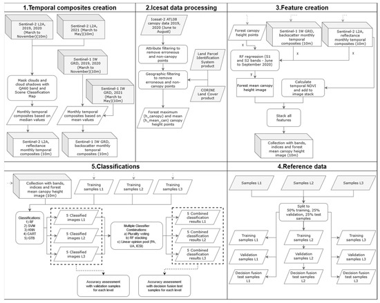
Figure 1.
Overall workflow of the study.
Thematic classification at all three levels relied on five individual classification algorithms (“base classifiers”): random forest (RF), support vector machines (SVM), k-nearest neighborhood (KNN), classification and regression trees (CART), and gradient tree boosting (GTB). The base classifiers were combined using three ensemble approaches for each level, forming a total of fifteen MCS classification experiments: (i) a simple plurality voting, (ii) a random forest meta-classifier, and (iii) three linear opinion pool algorithms using different accuracy metrics as weights.
All classification experiments used a “multiple” framework [12], relying on the use of multisource and multitemporal data. Monthly composites of Sentinel-1 and Sentinel-2 imagery were created in Step 1 (Figure 1). In Step 2, ICESat-2 photon counting data were filtered to remove erroneous and non-canopy footprints. In Step 3, the spatial explicit mean forest canopy and top canopy height variables (from the ICESat-2 footprint data) were upscaled and produced over the whole study area. Also, during Step 3, NDVI synthetic bands were produced and included in the classification experiments, along with all the original bands from the Sentinel-1 and Sentinel-2 temporal series.
In Step 4, the reference data for each level were split according to a 50–25–25 percentage ratio for training, validating the base classifiers, and evaluating the MSCs using appropriate measures. All algorithms were implemented on Google Earth Engine (GEE), a cloud platform that is freely provided for research purposes.
3. Study Area
The study area in Northeastern Greece extended over the five prefectures (Evros, Rodopi, Xanthi, Kavala and Drama) forming the Region of Eastern Macedonia and Thrace, and the Serres prefecture within the Region of Central Macedonia (Figure 2). The 17,585.13 km2 area includes many environmentally important sites and protected areas, such as the mountains of Rodopi, the National Park of the Dadia-Lefkimmi-Soufli Forest, the National Wetland Park of the Evros Delta, the Eastern Macedonia and Thrace National Park, the Rodopi Mountains National Park, and part of the Kerkini Lake National Park.
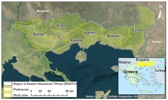
Figure 2.
Study area location and extent.
The annual temperature ranges from −14 °C to 38 °C, while precipitation during the summer period varies greatly from 80 to 120 mm in areas close to the coast and can be over 320 mm in the inland mountainous regions [32]. The vegetation zones found in the area are Quercion ilicis, Quercion confertae, Ostryo-Carpinion, Fagion moesiacae, Azonal–riparian, and Vacinio picetalia [33].
4. Data and Pre-Processing
4.1. Remote Sensing and Ancillary Data
The study relied in the use of satellite imagery from Sentinel-1 radar and Sentinel-2 optical missions, as well as LiDAR data from NASA’s ICESat-2 photon-counting Advanced Topographic Laser Altimeter System (ATLAS) instrument (Table 1). Sentinel-1 ground range-detected images and Sentinel-2 surface reflectance images (both at 10 m spatial resolution) were accessed in an analysis-ready data format through the GEE platform [34].

Table 1.
Details of the satellite data used in this study: namely, Sentinel-2, Sentinel-1, and ICESat-2 data.
Sentinel-2 L2A images—which contained the following bands: visible (B2 to B4), vegetation red edge (B5 to B7), near infrared (B8 and B8A) and shortwave infrared (B11 and B12)—acquired from March to November (2019 and 2020) and from March to May (2021) were retrieved to generate information about the temporal spectral profiles of all forest classes. Regarding the Sentinel-1 data, all images in ascending and descending order over the same date ranges as the Sentinel-2 images were also considered.
After filtering the ICESat data, it was determined that the number of available points within the study area for the months of May to September 2021 was insufficient. Therefore, it was decided that we would retain only the data from the years 2019 and 2020. Since we assume that there were no changes in vegetation during this period, for S1 and S2, data from May to September 2021 was used in order to create higher-quality composites.
To quantify vertical forest structure across the study area, the maximum (‘h_canopy’) and mean (‘h_mean_can’) canopy height estimates at each footprint point were obtained from the ICESat-2 ATL08 data repository for the June–August period (2019 and 2020) via the ‘icepyx’ library in python [35].
In addition to RS data, ancillary geospatial data were used to facilitate reference data selection and ICESat-2 pre-processing. The Greek “Land Parcel Identification System” (LPIS) [36] and the Copernicus CORINE Land Cover product (CLC 2018) [37] were used to identify ICESat-2 footprints over woody vegetation areas. Existing maps of tree species distribution (analog and digital) from 10-year forest management plans were gathered from local forest service departments within the study area. Finally, ESA’s IMAGE 2018 dataset, which provides very high-resolution (VHR) orthorectified multispectral products throughout Europe, and freely available very high-spatial-resolution basemaps from Google and Hellenic Cadastre, was used for visual interpretation purposes and reference data development.
4.2. Satellite Data Pre-Processing
Snow, cirrus, clouds, and cloud shadows were masked over the Sentinel-2 images using the scene classification map included in the L2A product. Monthly temporal composites based on the median pixel values were created, representing the median values of each pixel over the course of 9 months, resulting in nine synthetic monthly images [16,38]. In addition to the original Sentinel-2 temporal composites, an NDVI [39] value was calculated for each month. The creation of Sentinel-1 image composites was based on the minimum value instead of the median value, in order to overcome terrain and humidity effects [16].
The ICESat-2 data were filtered in order to remove erroneous and non-canopy points. More specifically, filters related to (i) land cover, (ii) cloud coverage, (iii) terrain and canopy height uncertainty, (iv) canopy height, (v) number of photons, and (vi) solar elevation were applied [40,41]. Spatial queries were additionally applied to remove points that (i) were outside the bounds of forest and seminatural areas (CLC 2018), (ii) were within 20 m distance of a water body (CLC 2018), and (iii) were within non-vegetated parcels included in the LPIS dataset. The number of points that resulted from the filtering and that were used for predicting canopy height in the next step was 782.
Subsequently, wall-to-wall maps of the top and mean canopy height across the study area were created using the ICESat-2 ‘ATL08 footprint data. Two RF regression models based upon Sentinel-1 and Sentinel-2 temporal composites (spanning from June to September 2019) were used for extrapolating the ICESat-2 footprint data. Each model’s accuracy was then evaluated based on Pearson’s correlation coefficient (R) and the coefficient of determination (R2), and the best-fitted models were used to extract the upscaled canopy height layers across the study area.
4.3. Classification Scheme and Reference Data
To assess the potential of MCSs for improving the accuracy of classifications for different levels of the spatial hierarchy within forest ecosystems, a multi-level classification approach was adopted (Table 2).
Table 2.
Classification scheme for the three levels and reference pixels for each class (in parentheses). The lower level of the hierarchy (L3) refers to individual tree species; the middle level (L2) refers to evergreen forests, deciduous forests, and shrubs; and the upper level (L1) includes the discrimination of woody vegetation (forest and shrubs) areas from other land.
Ground reference data were assembled using existing forest maps and intensive manual interpretation procedures using VHR imagery. Initially, we delineated as many “pure” polygons as possible with a high confidence level, which corresponded to spatial entities across the study area that were included in the nine classes of the lower level (L3) and the shrubs included in the middle level (L2). Additionally, to identify reference data for non-woody vegetation areas, the “pure” spatial entities of artificial surfaces, water, and barren and cultivated (annual/permanent) areas were delineated, taking into account the information about “within-class” variability provided by the CLC. In total, 5000 reference polygons for all levels were created. Subsequently, we generated random points within each polygon, considering a 30 m minimum distance among them, to minimize spatial autocorrelation while selecting an adequate number of points.
To formulate the training and testing sets, we followed a bottom-up approach. First, sample points were selected for each class in the lower level of the hierarchy (species). Next, evergreen and deciduous species samples were grouped together, and through proportional stratified random sampling, sample points for these two forest types were specified, equal to the available sample points for the shrub class. All individual tree species (L3) and shrub sample points (L2) were integrated into the forest and shrub class samples in the upper level (L1). Again, using proportional stratified random sampling, an equal number of non-woody vegetation samples were selected from the original pool of points of artificial surfaces, water, and barren and cultivated areas.
For each level of the hierarchy, the sample points were split into training, validation, and testing, using a 1 km grid created over the image to avoid spatial correlation [42]. For each class, 50% of the grid boxes were selected in a checkerboard manner for training, and the remaining 50% were further divided by 50% into validation and testing samples, creating a 50/25/25 percentage ratio.
5. Methodology
5.1. Base Classification Algorithms
The MCS framework used in the study employed five supervised, non-parametric classification algorithms or “base classifiers”. These included RF, SVM, KNN, CART, and GTB. RF [43] is a popular machine learning algorithm used in land use/land cover (LULC) applications. RF’s advantages include its robustness in the presence of outliers and noise, lower computational complexity compared to other ML methods, transparency, and ability to handle to a large number of variables and maintain a bias–variance tradeoff [44]. RF fits an ensemble of decision trees by randomly selecting a set of training samples and variables. The number of trees in the forest (Ntree) was set to 400, and the number of input variables randomly chosen at each split (Mtry) was set as the square root of the number of features [45,46].
SVM [47] is well-known for handling small sample sizes and producing high classification accuracies without overfitting [48]. In this study, the RBF kernel was chosen and the penalty parameter C and bandwidth parameter γ were set to 10 and 0.5, respectively.
The KNN classifier [49] is a simple and effective classification method that requires almost no parameter settings. This is a non-parametric classification technique where a class is determined based on the most frequent class among its ‘k’ nearest neighbors, with ‘k’ being a positive, usually small, integer value. If k equals 1, the pixel or object is classified according to the class of its nearest neighbor [50]. In the current study, KNN was implemented using the Mahalanobis distance, and k was set to 1 following the work of Qian et al. [51] and Thanh Noi and Kappas [52].
CART [53] generates binary decision trees by dividing the feature space of each sample into two sub-spaces until the terminal nodes of the developed trees are associated with a class [54]. The only parameters defined for the CART algorithm were the number of instances in a node below which the tree will not split (set to 5), while the maximum number of leaf nodes in each tree was given no limit.
GTB [55] is an ensemble machine learning technique that combines weak decision trees into a strong one through the boosting method. The number of decision trees and the rest of the parameters for GTB were set to the default GEE values (i.e., shrinkage: 0.005, sampling rate: 0.7, maximum number of leaf nodes in each tree: no limit).
5.2. Ensemble Approaches to Fusing the Base Classifiers
Following the individual-level classifications using single-base classifiers, three approaches were implemented for the combination of the classifiers: (i) a plurality voting algorithm, (ii) a random forest meta-classifier, and (iii) a linear opinion pool algorithm, integrating three different accuracy metrics as weights. The plurality voting algorithm is a commonly employed approach that selects the class label generated by the majority of classifiers for each pixel [56]:
where Li is the label assigned to pixel A by base classifier i.
A meta-classifier is another ensemble approach that utilizes the outputs of prior classifiers (base classifiers) as input features for a new classification. This technique is commonly referred to as “stacking” in literature. In our study, the RF classifier was employed as a meta-classifier, as described by Healey et al. [30].
The linear opinion pool (LOP) [57] is a general decision fusion method that is based on the weighted sum of class label probabilities obtained from each base classifier:
where LOP(A) is the combined probability from applying a set of classifiers to pixel A, αi is the weight given to the ith classifier, Pi(A) is the probability of the ith classifier for pixel A, and K is the number of classifiers. In our study, the LOP approach was implemented by incorporating three distinct accuracy metrics for each class: namely, the producer’s accuracy (PA), the user’s accuracy (UA), and the Individual Classification Success Index (ICSI). The combined probability value for each class label was calculated using Equation (2), and the resulting class label was determined based on the maximum value obtained for LOP(A).
5.3. Accuracy Assessment
To validate the performance of each of the five base classifiers, a common set of points corresponding to 25% of the reference dataset at each level was used to generate the confusion matrix and calculate the resulting accuracy measures: the overall accuracy (OA), PA, UA, and ‘kappa hat’ (Khat) values. In addition, the mean absolute differences (MAD) between PA and UA and the Individual Classification Success Index (ICSI) values were also considered. The ICSI is a combination of the PA and UA and accounts for the overall classification success for each class [58]. Finally, we calculated the macro-averaged F1 score as the average F1 score of the individual classes [59]. The class-level F1 score metric is calculated as the harmonic mean of UA and PA [60].
The same set of metrics was used to assess the accuracy of the MCS classification approaches based on an independent set of sample points (test data) corresponding to 25% of the reference dataset.
To evaluate the impact of base classifier output diversity on the accuracy of the MCS approach, a non-pairwise diversity measure based on entropy (E) was used. This measure calculated the diversity of the ensemble at each of the three levels [61].
where N is the sample size used from the L classifiers, ceil(L/2) rounds the given number of classifiers to the nearest integer, and h(xi) refers to classifiers among L that give the same output. The entropy measure ranges from 0 to 1, with 0 indicating no difference among the classifiers and 1 indicating the highest possible diversity value.
6. Results
The OA and the Khat values of the individual base classifiers were evaluated across the entire study area, and the results are presented in Table 3 and Figure 3, while the detailed error matrices are given in the Supplementary Materials. The highest accuracy for discriminating forest and shrubs from other land areas at the upper level (L1) was achieved using the RF and SVM algorithms, with OA values of 92.71% and 92.34%, respectively.
Table 3.
Overall classification accuracy (in %) with 95% confidence interval (in parentheses) for the 10 classification experiments across each hierarchical level. Results are shown for both the five individual base classifiers and the five MCS approaches.
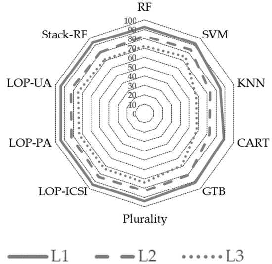
Figure 3.
Overall accuracy of the base classifiers and MCSs for each hierarchical level. The upper, abstract level (L1) demonstrates higher accuracy rates, whereas the increased classification scheme complexity in the lower level (L3) leads to reduced accuracies.
It appears that the CART-based approach had the lowest OA among the individual base classifiers, with an accuracy of 88.49%. However, all of the five MCS approaches that were employed showed a slight improvement in classification accuracy compared to the RF algorithm, with OA values close to 94.00%. This represents an improvement of approximately 1.00% compared to the best-performing individual base classifier, which was the RF algorithm.
At the middle level of the hierarchy (L2), the OA obtained from the base classifiers (Figure 3 and Table 3) is lower compared to the upper level (L1). The middle level of the hierarchy (L2) exhibits a wider range of individual accuracies compared to the upper level (L1), spanning from 72.61% (CART) to 84.13% (SVM) (Table 3). The range of OA values for the five ensembles considered within the MCS framework to discriminate deciduous forests, evergreen forests, and shrubs in L2 is greater than the MCS accuracy results for the binary class scheme of the upper level (L1).The RF stacking MCS approach produced the lowest accuracy (80.75%), while the LOP approach using the ICSI metric (LOP-ICSI) generated the highest accuracy (83.55%), albeit slightly lower than the SVM approach’s accuracy.
In contrast, the lower level for tree species composition discrimination (L3) resulted in even lower OA compared to the other two levels of the hierarchy, for both the individual and the ensemble classification approaches. The KNN classifier presented the lowest OA (58.22%), followed by the CART classifier (58.82%). However, SVM (OA = 74.89%) outperformed all the individual base classifiers. For the MCS approach, once again, the Stack-RF approach had a low OA (71.78%), while the LOP approach using the UA measure (LOP-UA) achieved the highest accuracy (74.61%).
The entropy diversity measure calculated for the results of the individual base classifiers in all three levels confirmed the differences observed in the OA of the classifiers. Higher entropy (0.31) was noted in the lower level (L3), where the range of the OA classification accuracy noted between classifiers was almost 15%. Lower entropy values were noted in the middle level (0.19) and upper level (0.08) of the hierarchy (Figure 4).
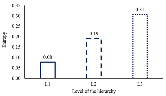
Figure 4.
Entropy measurement for the individual classification outcomes from the five base classifiers used in the MCSs. A higher entropy is observed for the lower level (L3).
In terms of PA at the upper level (L1), the SVM (PA = 94.59%) and GTB (PA = 95.46%) algorithms show the lowest commission error for forests and shrubs, while the KNN algorithm (PA = 74.00%) exhibits the highest (Figure 5). On the other hand, the algorithms with the highest commission errors are the GTB (UA = 89.12%) and CART (UA = 87.95%) approaches. All five ensemble approaches produce the same balanced omission and commission errors (PA = 94%, UA = 94%), as indicated by their high and equal ICSI scores (88.00%).
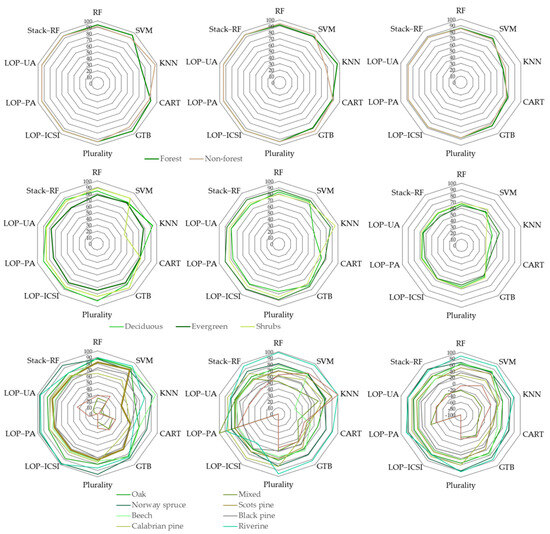
Figure 5.
Class-specific accuracy metrics displayed for each hierarchical level. The columns, from left to right, represent PA, UA, and ICSI. The rows, from top to bottom, correspond to the L1, L2, and L3 hierarchical levels. Results are presented for both the five individual base classifiers and the five MCS approaches.
At the middle level of the hierarchy, the SVM and CART base classifiers exhibit lower MAD values, indicating a better balance of commission and omission errors. The SVM classifier achieved high classification success (average ICSI = 68%), and CART presented the lowest mean ICSI (45.00%). On the other hand, the KNN base classifier has the highest MAD (30.67%) and a very low average ICSI (52.67%). Among the MCS approaches, the LOP-UA ensemble performs the best (MAD = 6% and average ICSI = 66.33%), while the Stack-RF approach yields the least satisfactory results (MAD = 10% and average ICSI = 62.33%).
At the lower level of the hierarchy (L3), SVM is the most balanced classifier in terms of omission and commission errors, with an average MAD of 14.67%. In contrast, the CART classifier performs poorly, with an average ICSI of 13.78%. In the L3 evaluations of MCS approaches, LOP-UA yielded the most satisfactory individual class accuracies, recording an MAD of 15.11% and an ICSI of 40.11%.
The efficacy of the MCS approach is underscored by the macro-averaged F1 scores from both the LOP-UA and plurality systems. Impressively, these scores surpassed those of the SVM and RF classifiers across all hierarchical levels, as shown in Table 4. Specifically, at the upper level of the hierarchy, LOP-UA and LOP-ICSI both achieved a macro-averaged F1 score of 98.56%, marginally trailing the plurality approach at 98.72%. Conversely, for individual base algorithms, RF (92.69%) and SVM (92.31%) presented the highest macro-averaged F1 scores among the five algorithms, signaling balanced class accuracy.
Table 4.
Macro-averaged F1 scores (%) attained for the 10 classification experiments over each level of the hierarchy, both for individual base classifiers and MCS approaches. The MCS approaches, based on linear opinion pool using user’s accuracy (LOP-UA) and plurality, outperformed all other classification experiments.
At the middle hierarchical level, every MCS approach, except for the Stack-RF approach, resulted in an average F1 score above 92%, markedly exceeding the SVM’s 84.19% and RF’s 82.84%.
Lastly, at the more detailed L3 level, both LOP UA (80.87%) and plurality (80.63%) replicated their L2 performance, showcasing an improvement of approximately 8% over the SVM (71.71%) and RF (68.87%) base algorithms.
When comparing the resulting map with those generated by the other four base classifiers (Figure 6), it is evident that the KNN algorithm shows a high omission error (PA = 74.01%) in the discrimination of forest and shrubs.
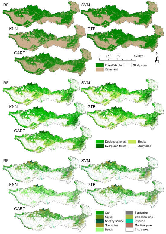
Figure 6.
Forest maps generated by the base classifiers for each hierarchical level. It is evident that the KNN algorithm underperforms across all levels.
Upon closer examination of the individual classifications at the middle and lower levels of the hierarchy (Figure 7 and Figure 8), it becomes clear that differences in numerical accuracy also correspond to variations in spatially explicit class distribution. At both levels, the maps generated from the MCSs are highly consistent with the one produced by the best-performing individual base classifier (i.e., SVM).
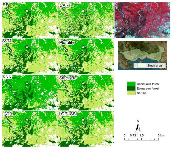
Figure 7.
Close-up view of the L2 classification results for both the base classifiers and MCSs. The maps produced using the MCSs align closely with the output of the SVM classifier.
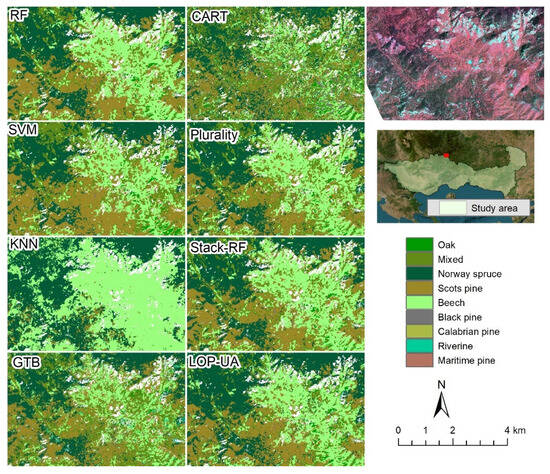
Figure 8.
Close-up view of the L3 classification results for both base classifiers and MCSs. The maps produced using the Multiple Classifier Systems (MCSs) approach align closely with the output of the Support Vector Machine (SVM) classifier.
Conversely, the maps produced through the CART classifier at both levels exhibit a significant “salt and pepper” effect. Furthermore, the magnitude of errors observed in the KNN accuracy assessment results is also apparent in the corresponding maps when compared to satellite imagery.
7. Discussion
In our study, we evaluated individual classifiers and multi-classifier systems (MCSs) for forest information extraction across different levels of forest hierarchy in Northern Greece using a Google Earth Engine workflow. Our best-performing individual classifier for discrimination of forest and shrubs from other land (L1) was the RF algorithm, achieving an OA of 92.71%, slightly higher than the SVM algorithm’s accuracy of 92.31%. In comparison, previous studies have reported even higher accuracies using RF for forest/non-forest classification with Sentinel-2 time series data, such as 98% in the Polish Carpathian Mountains [62] and 98.3% in Southern Poland [63], as well as 98% in a less complex terrain in Denmark [64] using multi-temporal passive and active Sentinel data. However, this might be related to the higher biological and structural diversity of Mediterranean forest ecosystems resulting from the environmental characteristics of the region and the long-term human impact [65].
The good performance of RF in terms classification accuracy, along with its low requirements in terms of hyperparameter tuning and rather low computational costs, justifies its popularity within the RS community for large scale applications [66]. RF, being an ensemble classifier, aggregates results from numerous decision trees. This allows it to model complex classification tasks better, reducing the chances of overfitting. The inherently random nature of this classifier, where it randomly selects features for each tree, can enhance the robustness of its classifications.
Although SVM was not the best-performing algorithm for forest and shrub discrimination in L1, it outperformed RF in the discrimination of forest types at L2 (OA = 84.13%) and in forest species classification at L3 (OA = 74.89%). In a straightforward binary classification problem within a bidimensional feature space, an SVM would typically fit a straight line as the optimal separating plane. However, when dealing with multiple classes that exhibit high spectral similarity and are not linearly separable, it becomes essential to introduce extra variables. These variables, known as slack variables, are incorporated into SVM optimization using the soft margin method, allowing for some classification errors [67]. In addition, the essence of the kernel trick lies in projecting the feature space to a higher-dimensional space (like Euclidean or Hilbert) to enhance the separability of classes [44].
Other studies have reported higher accuracies for these levels of the hierarchy. For instance, Bjerreskov et al. [64] achieved a 95% OA for mapping broadleaved and coniferous forests in Denmark, similar to the findings of Hościło and Lewandows in Southern Poland [63]. Wessel et al. [68], who also used multitemporal Sentinel-2 data and an SVM classifier, discriminated coniferous from broad-leaved trees, achieving a 97% OA in Bavaria, Germany. We hypothesize that the lower accuracies observed in our study may be attributed to forest heterogeneity and the inclusion of a shrubland class in the middle level of the hierarchy. Classes based on forests and shrublands are frequently misidentified during image classification. This confusion arises from similar species compositions (especially in the case of early successional forests), which vary primarily in plant height or canopy formation, thus making necessary the use of information such as that provided by airborne LiDAR datasets for their discrimination [69].
In terms of forest species classification at L3, our study found that the SVM classifier performed satisfactorily, achieving an OA that was comparable to the results obtained by Bjerreskov et al. [64], who used the RF classifier (OA = 63% in the discrimination of six forest species). However, Grabska et al. [20] achieved a higher OA of 87% for forest species mapping in the Polish Carpathian Mountains using Sentinel-2 imagery and an SVM, with a more complex class scheme consisting of eleven forest species. Our study also demonstrated the inferiority of the CART algorithm, as was also explored in Nasiri et al.’s [54] study on tree species identification in a temperate Caspian forest. The CART algorithm it has advantages in terms of the transparency of the results, speed, and ease of use [70]. However, the partitioning of the feature space into many independent regions and the fact that final classification output is generated by hard boundary decisions at every node may result in lower accuracies compared to other machine learning algorithms [71].
Our findings are consistent with those of Maxwell et al. [22], who emphasize that there is no one-size-fits-all machine learning algorithm and that the best approach depends on the specific class scheme, the type of training data, and the RS data used. However, it is worth noting that the largest difference in accuracy (i.e., 2.9%) was observed at the lowest level of the hierarchy (L3), where the training data were highly imbalanced. RF algorithms have been shown to struggle with imbalanced training data [22,68], whereas SVM may perform better in such situations [72]. Also, SVM is more efficient in finding decision limits for classifying objects with greater spectral similarity because of its ability to identify the decision borders and expand the space between them, even when using limited training datasets [54]. This is accomplished due to the soft margin and kernel trick to map the feature space into a higher dimension for improving the separability between classes [73]. However, decision tree learning techniques such as CART and RF are advantageous in terms of interpretability and simplicity, contrary to other algorithms (i.e., SVM, NN) that are characterized as “black box” algorithms [22].
In RS image classification, MCSs have been proposed as a means to improve the accuracy and reduce the variance in classification results [29]. However, studies have shown mixed results regarding the effectiveness of MCSs, with some reporting only slight improvements compared to the best individual classifiers [20,24], while others demonstrate significant increases of up to 6% in classification accuracy [74,75,76]. Based on the findings of this study, it appears that the use of MCSs only marginally improved the OA by 1.2% in the L1 case, while in L2 and L3, the best MCS achieved slightly lower accuracy compared to the most accurate base classifier (SVM). The lack of classifier diversity could be a possible explanation for the marginal or lack of improvement in OA, as diversity is an important parameter for the improvement of classification accuracy via MCSs. Previous studies have demonstrated that the success of any MCS is related to the accuracy and diversity of the base classifiers included in the system [74]. Thus, an ensemble of classifiers could improve the accuracy of any of its individual members if they have a low error rate (are accurate) and their errors are not coincident (are diverse). Obtaining base learners which satisfy both requirements simultaneously is not an easy task because the lower the number of errors, the higher its correlation is [77]. It is worth noting that in the more diverse L3, unlike L1, none of the MCS approaches outperformed the SVM base classifier in terms of OA. This mirrors the findings of an earlier study [31].
Yet, while the PA and UA of the base classifiers varied significantly among classes, the MCSs had more robust performance among classes in most cases, especially at levels one and three, except for two specific categories in L3—namely, “mixed forest” and “Maritime pine”—likely due to the high within-class spectral variability. Nevertheless, improvement in per-class accuracy with the use of MCS has been reported in the literature [78], indicating that despite a marginal increase in OA, MCS can balance class accuracy differences. While in some applications—for example, binary class mapping—imbalanced balanced class accuracies might be advantageous for classification map quality fine-tuning [79], in forest management, balanced accuracy among classes is usually advantageous since this can limit uncertainty in forest management models and subsequent decisions.
The evaluation of the macro-averaged F1 scores suggests that the MCS approach generally enhances classification stability. Notably, the plurality and LOP-UA MCS approaches consistently outperformed the base algorithms across all levels of the forest’s hierarchy. The macro-averaged F1 score is deemed a more suitable metric when assessing the accuracy of maps that display an unbalanced class distribution [59]. Previous research has highlighted that, despite its simplicity, plurality voting is beneficial for merging the results of base classifiers [78]. Conversely, while approaches like LOP-UA, which weigh votes based on accuracy metrics, can be effective, they may encounter stability or transferability issues when applied across different biophysical covers [28].
8. Conclusions
The study assessed the performance of MCSs in comparison to individual base classifiers for forest information extraction at three different levels of forest hierarchy in a Mediterranean region. The results showed that the use of MCS marginally improved OA in the L1 case, but in L2 and L3, the best MCS achieved slightly lower accuracy compared to the best-performing base classifier.
While there were high fluctuation rates in the OA measures for each classification in the different base classifiers, the MCS experiments showed lower rates of fluctuation. The MCSs also had more robust performance among classes, especially in levels one and three, improving per-class accuracy and balancing class accuracy differences. Overall, while MCSs may not always outperform individual base classifiers, they can provide more robust performance among classes and balance class accuracy differences.
While this study contributes valuable insights to the application of multiple classifier systems (MCSs) for multi-scale forest mapping, there are a few limitations that must be acknowledged. Firstly, the optimization of the individual base algorithms was not conducted, which could potentially lead to improved accuracy in future studies. Secondly, the findings of this study were based solely on an examination of Northeastern Greece. An exploration of other geographical areas could provide a more comprehensive understanding of the applicability and effectiveness of the MCS approach in diverse settings. As such, further research should consider these limitations in order to further enhance our understanding of forest mapping using RS data.
Supplementary Materials
The following supporting information can be downloaded at https://www.mdpi.com/article/10.3390/f14112224/s1: Table S1: Error matrices for the L1 base and ensemble classifiers; Table S2: Error matrices for the L2 base and ensemble classifiers; Table S3: Error matrices for the L3 base and ensemble classifiers.
Author Contributions
Conceptualization, G.M.; methodology, G.M., S.S. and N.V.; software, N.V. and S.S.; validation, G.M., S.S. and N.V.; data curation, D.L. and C.A.; writing—original draft preparation, G.M., N.V. and S.S.; writing—review and editing, G.M., D.L., C.A. and I.K.; supervision, G.M.; project administration, I.K.; funding acquisition, I.K. All authors have read and agreed to the published version of the manuscript.
Funding
This work was supported by the Eye4Water project, MIS 5047246, implemented under the action “Support for Research Infrastructure and Innovation” by the Operational Program “Competitiveness, Entrepreneurship and Innovation”, which was co-financed by Greece and the European Union’s European Regional Development Fund.
Data Availability Statement
The data presented in this study are available upon request from the corresponding author.
Acknowledgments
Sentinel-1 and Sentinel-2 data used were available at no cost from ESA Sentinels Scientific Data Hub. Figure 6, Figure 7 and Figure 8 contain modified Copernicus Sentinel data (2020). The authors are also grateful to the General Secretariat of Forests, General Directorate for Forests and Forest Environment, Ministry of Environment and Energy (Greece) for providing the regional forest maps. We thank the two anonymous reviewers whose insightful comments helped to substantially improve this manuscript. In addition, we would like to thank Eleni Papadopoulou for her support in preparing the revised version of this manuscript.
Conflicts of Interest
The authors declare no conflict of interest.
References
- FAO; UNEP. The State of the World’s Forests 2020: Forests, Biodiversity and People; FAO: Rome, Italy, 2020. [Google Scholar]
- FAO; Plan Bleu. State of Mediterranean Forests 2018; FAO: Rome, Italy, 2018; ISBN 978-92-5-131047-2. [Google Scholar]
- Fassnacht, F.E.; White, J.C.; Wulder, M.A.; Næsset, E. Remote sensing in forestry: Current challenges, considerations and directions. For. An Int. J. For. Res. 2023, 2023, cpad024. [Google Scholar] [CrossRef]
- Lechner, A.M.; Foody, G.M.; Boyd, D.S. Applications in Remote Sensing to Forest Ecology and Management. One Earth 2020, 2, 405–412. [Google Scholar] [CrossRef]
- Fernandez-Carrillo, A.; Franco-Nieto, A.; Pinto-Bañuls, E.; Basarte-Mena, M.; Revilla-Romero, B. Designing a Validation Protocol for Remote Sensing Based Operational Forest Masks Applications. Comparison of Products Across Europe. Remote Sens. 2020, 12, 3159. [Google Scholar]
- Fassnacht, F.E.; Latifi, H.; Stereńczak, K.; Modzelewska, A.; Lefsky, M.; Waser, L.T.; Straub, C.; Ghosh, A. Review of studies on tree species classification from remotely sensed data. Remote Sens. Environ. 2016, 186, 64–87. [Google Scholar] [CrossRef]
- Konrad, T.; Ozdogan, M.; Radeloff, V.C. Mapping forest types over large areas with Landsat imagery partially affected by clouds and SLC gaps. Int. J. Appl. Earth Obs. Geoinf. 2022, 107, 102689. [Google Scholar]
- Franklin, S.E. Remote Sensing for Sustainable Forest Management; CRC Press: Boca Raton, FL, USA, 2001; ISBN 1-56670-394-8. [Google Scholar]
- Pekkarinen, A.; Reithmaier, L.; Strobl, P. Pan-European forest/non-forest mapping with Landsat ETM+ and CORINE Land Cover 2000 data. ISPRS J. Photogramm. Remote Sens. 2009, 64, 171–183. [Google Scholar] [CrossRef]
- Schwaab, J.; Davin, E.L.; Bebi, P.; Duguay-Tetzlaff, A.; Waser, L.T.; Haeni, M.; Meier, R. Increasing the broad-leaved tree fraction in European forests mitigates hot temperature extremes. Sci. Rep. 2020, 10, 14153. [Google Scholar] [CrossRef]
- Xiao, Q.; Ustin, S.L.; McPherson, E.G. Using AVIRIS data and multiple-masking techniques to map urban forest tree species. Int. J. Remote Sens. 2004, 25, 5637–5654. [Google Scholar] [CrossRef]
- Pu, R. Mapping Tree Species Using Advanced Remote Sensing Technologies: A State-of-the-Art Review and Perspective. J. Remote Sens. 2021, 2021, 9812624. [Google Scholar] [CrossRef]
- Waser, L.T.; Rüetschi, M.; Psomas, A.; Small, D.; Rehush, N. Mapping dominant leaf type based on combined Sentinel-1/-2 data – Challenges for mountainous countries. ISPRS J. Photogramm. Remote Sens. 2021, 180, 209–226. [Google Scholar] [CrossRef]
- Rüetschi, M.; Small, D.; Waser, L.T. Rapid detection of windthrows using Sentinel-1 C-band SAR data. Remote Sens. 2019, 11, 115. [Google Scholar] [CrossRef]
- Rüetschi, M.; Weber, D.; Koch, T.L.; Waser, L.T.; Small, D.; Ginzler, C. Countrywide mapping of shrub forest using multi-sensor data and bias correction techniques. Int. J. Appl. Earth Obs. Geoinf. 2021, 105, 102613. [Google Scholar] [CrossRef]
- Theofanous, N.; Chrysafis, I.; Mallinis, G.; Domakinis, C.; Verde, N.; Siahalou, S. Aboveground Biomass Estimation in Short Rotation Forest Plantations in Northern Greece Using ESA’s Sentinel Medium-High Resolution Multispectral and Radar Imaging Missions. Forests 2021, 12, 902. [Google Scholar] [CrossRef]
- Simard, M.; Pinto, N.; Fisher, J.B.; Baccini, A. Mapping forest canopy height globally with spaceborne lidar. J. Geophys. Res. Biogeosciences 2011, 116. [Google Scholar] [CrossRef]
- Hamedianfar, A.; Mohamedou, C.; Kangas, A.; Vauhkonen, J. Deep learning for forest inventory and planning: A critical review on the remote sensing approaches so far and prospects for further applications. For. An Int. J. For. Res. 2022, 95, 451–465. [Google Scholar] [CrossRef]
- Zhang, C.; Liu, Y.; Tie, N. Forest Land Resource Information Acquisition with Sentinel-2 Image Utilizing Support Vector Machine, K-Nearest Neighbor, Random Forest, Decision Trees and Multi-Layer Perceptron. Forests 2023, 14, 254. [Google Scholar] [CrossRef]
- Grabska, E.; Frantz, D.; Ostapowicz, K. Evaluation of machine learning algorithms for forest stand species mapping using Sentinel-2 imagery and environmental data in the Polish Carpathians. Remote Sens. Environ. 2020, 251, 112103. [Google Scholar] [CrossRef]
- Mallinis, G.; Koutsias, N.; Tsakiri-Strati, M.; Karteris, M. Object-based classification using Quickbird imagery for delineating forest vegetation polygons in a Mediterranean test site. ISPRS J. Photogramm. Remote Sens. 2008, 63, 237–250. [Google Scholar] [CrossRef]
- Maxwell, A.E.; Warner, T.A.; Fang, F. Implementation of machine-learning classification in remote sensing: An applied review. Int. J. Remote Sens. 2018, 39, 2784–2817. [Google Scholar] [CrossRef]
- Schulz, D.; Yin, H.; Tischbein, B.; Verleysdonk, S.; Adamou, R.; Kumar, N. Land use mapping using Sentinel-1 and Sentinel-2 time series in a heterogeneous landscape in Niger, Sahel. ISPRS J. Photogramm. Remote Sens. 2021, 178, 97–111. [Google Scholar] [CrossRef]
- Man, C.D.; Nguyen, T.T.; Bui, H.Q.; Lasko, K.; Nguyen, T.N.T. Improvement of land-cover classification over frequently cloud-covered areas using Landsat 8 time-series composites and an ensemble of supervised classifiers. Int. J. Remote Sens. 2018, 39, 1243–1255. [Google Scholar] [CrossRef]
- Smits, P.C. Multiple classifier systems for supervised remote sensing image classification based on dynamic classifier selection. IEEE Trans. Geosci. Remote Sens. 2002, 40, 801–813. [Google Scholar] [CrossRef]
- Doan, H.T.X.; Foody, G.M. Increasing soft classification accuracy through the use of an ensemble of classifiers. Int. J. Remote Sens. 2007, 28, 4609–4623. [Google Scholar] [CrossRef]
- Zuev, Y.A. A probability model of a committee of classifiers. USSR Comput. Math. Math. Phys. 1986, 26, 170–179. [Google Scholar] [CrossRef]
- Shen, H.; Lin, Y.; Tian, Q.; Xu, K.; Jiao, J. A comparison of multiple classifier combinations using different voting-weights for remote sensing image classification. Int. J. Remote Sens. 2018, 39, 3705–3722. [Google Scholar] [CrossRef]
- Dou, P.; Shen, H.; Li, Z.; Guan, X. Time series remote sensing image classification framework using combination of deep learning and multiple classifiers system. Int. J. Appl. Earth Obs. Geoinf. 2021, 103, 102477. [Google Scholar] [CrossRef]
- Healey, S.P.; Cohen, W.B.; Yang, Z.; Kenneth Brewer, C.; Brooks, E.B.; Gorelick, N.; Hernandez, A.J.; Huang, C.; Joseph Hughes, M.; Kennedy, R.E.; et al. Mapping forest change using stacked generalization: An ensemble approach. Remote Sens. Environ. 2018, 204, 717–728. [Google Scholar]
- Vasilakos, C.; Kavroudakis, D.; Georganta, A. Machine learning classification ensemble of multitemporal Sentinel-2 images: The case of a mixed mediterranean ecosystem. Remote Sens. 2020, 12, 2005. [Google Scholar] [CrossRef]
- Hellenic Agency for Local Development and Local Government Longterm Strategic Plan of Sustainable Development East Macedonia and Thrace Region 2013. Available online: http://www.pedamth.gr/files/ArticleID/174/MakroprothesmoPAMTH.pdf (accessed on 1 September 2023).
- Spanos, K.; Gaitanis, D.; Skouteri, A.; Petrakis, P.; Meliadis, I. Implementation of Forest Policy in Greece in Relation to Biodiversity and Climate Change. Open J. Ecol. 2018, 8, 174–191. [Google Scholar] [CrossRef][Green Version]
- Earth Engine Data Catalog. Sentinel-2 MSI: MultiSpectral Instrument, Level-2A. Available online: https://developers.google.com/earth-engine/datasets/catalog/COPERNICUS_S2_SR (accessed on 1 September 2023).
- Neuenschwander, A.L.; Pitts, K.L. ICE, CLOUD, and Land Elevation Satellite (ICESat-2) Algorithm Theoretical Basis Document (ATBD) for Land—Vegetation Along-Track Products (ATL08); National Aeronautics and Space Administration: Washington, DC, USA, 2021.
- European Court of Auditors. The Land Parcel Identification System: A Useful Tool to Determine the Eligibility of Agricultural Land—But Its Management Could Be Further Improved; Publications Office: Luxembourg, 2016. [Google Scholar]
- Büttner, G. CORINE land cover and land cover change products. Remote Sens. Digit. Image Process. 2014, 18, 55–74. [Google Scholar]
- Griffiths, P.; Nendel, C.; Hostert, P. Intra-annual reflectance composites from Sentinel-2 and Landsat for national-scale crop and land cover mapping. Remote Sens. Environ. 2019, 220, 135–151. [Google Scholar] [CrossRef]
- Tucker, C.J. Red and photographic infrared linear combinations for monitoring vegetation. Remote Sens. Environ. 1979, 8, 127–150. [Google Scholar] [CrossRef]
- Jiang, F.; Zhao, F.; Ma, K.; Li, D.; Sun, H. Mapping the Forest Canopy Height in Northern China by Synergizing ICESat-2 with Sentinel-2 Using a Stacking Algorithm. Remote Sens. 2021, 13, 1535. [Google Scholar] [CrossRef]
- Tian, X.; Shan, J. Comprehensive Evaluation of the ICESat-2 ATL08 Terrain Product. IEEE Trans. Geosci. Remote Sens. 2021, 59, 8195–8209. [Google Scholar] [CrossRef]
- Karakizi, C.; Karantzalos, K.; Vakalopoulou, M.; Antoniou, G. Detailed Land Cover Mapping from Multitemporal Landsat-8 Data of Different Cloud Cover. Remote Sens. 2018, 10, 1214. [Google Scholar] [CrossRef]
- Breiman, L. Random forests. Mach. Learn. 2001, 45, 5–32. [Google Scholar] [CrossRef]
- Sheykhmousa, M.; Mahdianpari, M.; Ghanbari, H.; Mohammadimanesh, F.; Ghamisi, P.; Homayouni, S. Support Vector Machine Versus Random Forest for Remote Sensing Image Classification: A Meta-Analysis and Systematic Review. IEEE J. Sel. Top. Appl. Earth Obs. Remote Sens. 2020, 13, 6308–6325. [Google Scholar] [CrossRef]
- Chrysafis, I.; Mallinis, G.; Siachalou, S.; Patias, P. Assessing the relationships between growing stock volume and Sentinel-2 imagery in a Mediterranean forest ecosystem. Remote Sens. Lett. 2017, 8, 508–517. [Google Scholar] [CrossRef]
- Verde, Ν.; Kokkoris, I.; Georgiadis, C.; Kaimaris, D.; Dimopoulos, P.; Mitsopoulos, I.; Mallinis, G. National scale land cover classification for ecosystem services mapping and assessment, using multitemporal copernicus EO data and google earth engine. Remote Sens. 2020, 12, 3303. [Google Scholar] [CrossRef]
- Vapnik, V.N. The Nature of Statistical Learning Theory, 2nd ed.; Springer: New York, NY, USA, 2000; Volume 8, ISBN 978-1-4419-3160-3. [Google Scholar]
- Mountrakis, G.; Im, J.; Ogole, C. Support vector machines in remote sensing: A review. ISPRS J. Photogramm. Remote Sens. 2011, 66, 247–259. [Google Scholar] [CrossRef]
- Duda, R.O.; Hart, P.E. Pattern Classification and Scene Analysis; Wiley: New York, NY, USA, 1973. [Google Scholar]
- Orusa, T.; Cammareri, D.; Borgogno Mondino, E. A Scalable Earth Observation Service to Map Land Cover in Geomorphological Complex Areas beyond the Dynamic World: An Application in Aosta Valley (NW Italy). Appl. Sci. 2023, 13, 390. [Google Scholar] [CrossRef]
- Qian, Y.; Zhou, W.; Yan, J.; Li, W.; Han, L. Comparing Machine Learning Classifiers for Object-Based Land Cover Classification Using Very High Resolution Imagery. Remote Sens. 2014, 7, 153–168. [Google Scholar] [CrossRef]
- Thanh Noi, P.; Kappas, M. Comparison of Random Forest, k-Nearest Neighbor, and Support Vector Machine Classifiers for Land Cover Classification Using Sentinel-2 Imagery. Sensors 2018, 18, 18. [Google Scholar] [CrossRef]
- Breiman, L.; Friedman, J.; Stone, C.J.; Olshen, R.A. Classification and Regression Trees; Chapman & Hall: New York, NY, USA, 1984. [Google Scholar]
- Nasiri, V.; Beloiu, M.; Asghar Darvishsefat, A.; Griess, V.C.; Maftei, C.; Waser, L.T. Mapping tree species composition in a Caspian temperate mixed forest based on spectral-temporal metrics and machine learning. Int. J. Appl. Earth Obs. Geoinf. 2023, 116, 103154. [Google Scholar] [CrossRef]
- Friedman, J.H. Stochastic gradient boosting. Comput. Stat. Data Anal. 2002, 38, 367–378. [Google Scholar] [CrossRef]
- Clinton, N.; Yu, L.; Gong, P. Geographic stacking: Decision fusion to increase global land cover map accuracy. ISPRS J. Photogramm. Remote Sens. 2015, 103, 57–65. [Google Scholar] [CrossRef]
- Guan, X.; Liu, G.; Huang, C.; Liu, Q.; Wu, C.; Jin, Y.; Li, Y. An Object-Based Linear Weight Assignment Fusion Scheme to Improve Classification Accuracy Using Landsat and MODIS Data at the Decision Level. IEEE Trans. Geosci. Remote Sens. 2017, 55, 6989–7002. [Google Scholar] [CrossRef]
- Koukoulas, S.; Blackburn, G.A. Introducing new indices for accuracy evaluation of classified images representing semi-natural woodland environments. Photogramm. Eng. Remote Sensing 2001, 67, 499–510. [Google Scholar]
- Zhong, L.; Hu, L.; Zhou, H. Deep learning based multi-temporal crop classification. Remote Sens. Environ. 2019, 221, 430–443. [Google Scholar] [CrossRef]
- Foody, G.M. Challenges in the real world use of classification accuracy metrics: From recall and precision to the Matthews correlation coefficient. PLoS ONE 2023, 18, e0291908. [Google Scholar] [CrossRef] [PubMed]
- Du, P.; Xia, J.; Zhang, W.; Tan, K.; Liu, Y.; Liu, S. Multiple Classifier System for Remote Sensing Image Classification: A Review. Sensors 2012, 12, 4764–4792. [Google Scholar] [CrossRef] [PubMed]
- Grabska, E.; Hostert, P.; Pflugmacher, D.; Ostapowicz, K. Forest stand species mapping using the sentinel-2 time series. Remote Sens. 2019, 11, 1197. [Google Scholar] [CrossRef]
- Hościło, A.; Lewandowska, A. Mapping Forest Type and Tree Species on a Regional Scale Using Multi-Temporal Sentinel-2 Data. Remote Sens. 2019, 11, 929. [Google Scholar] [CrossRef]
- Bjerreskov, K.S.; Nord-Larsen, T.; Fensholt, R. Classification of Nemoral Forests with Fusion of Multi-Temporal Sentinel-1 and 2 Data. Remote Sens. 2021, 13, 950. [Google Scholar] [CrossRef]
- Scarascia-Mugnozza, G.; Oswald, H.; Piussi, P.; Radoglou, K. Forests of the Mediterranean region: Gaps in knowledge and research needs. For. Ecol. Manage. 2000, 132, 97–109. [Google Scholar] [CrossRef]
- Belgiu, M.; Drăgu, L.; Drăguţ, L. Random forest in remote sensing: A review of applications and future directions. ISPRS J. Photogramm. Remote Sens. 2016, 114, 24–31. [Google Scholar] [CrossRef]
- Rodriguez-Galiano, V.F.; Chica-Rivas, M. Evaluation of different machine learning methods for land cover mapping of a Mediterranean area using multi-seasonal Landsat images and Digital Terrain Models. Int. J. Digit. Earth 2014, 7, 492–509. [Google Scholar] [CrossRef]
- Wessel, M.; Brandmeier, M.; Tiede, D. Evaluation of Different Machine Learning Algorithms for Scalable Classification of Tree Types and Tree Species Based on Sentinel-2 Data. Remote Sens. 2018, 10, 1419. [Google Scholar] [CrossRef]
- Adams, B.T.; Matthews, S.N. Enhancing Forest and Shrubland Mapping in a Managed Forest Landscape with Landsat–LiDAR Data Fusion. Nat. Areas J. 2018, 38, 402–418. [Google Scholar] [CrossRef]
- Chirici, G.; Scotti, R.; Montaghi, A.; Barbati, A.; Cartisano, R.; Lopez, G.; Marchetti, M.; Mcroberts, R.E.; Olsson, H.; Corona, P. Stochastic gradient boosting classification trees for forest fuel types mapping through airborne laser scanning and IRS LISS-III imagery. Int. J. Appl. Earth Obs. Geoinf. 2013, 25, 87–97. [Google Scholar] [CrossRef]
- Shao, Y.; Lunetta, R.S. Comparison of support vector machine, neural network, and CART algorithms for the land-cover classification using limited training data points. ISPRS J. Photogramm. Remote Sens. 2012, 70, 78–87. [Google Scholar] [CrossRef]
- Heydari, S.S.; Mountrakis, G. Effect of classifier selection, reference sample size, reference class distribution and scene heterogeneity in per-pixel classification accuracy using 26 Landsat sites. Remote Sens. Environ. 2018, 204, 648–658. [Google Scholar] [CrossRef]
- Kavzoglu, T.; Colkesen, I. A kernel functions analysis for support vector machines for land cover classification. Int. J. Appl. Earth Obs. Geoinf. 2009, 11, 352–359. [Google Scholar] [CrossRef]
- Zhang, P.; Hu, S.; Li, W.; Zhang, C.; Cheng, P. Improving parcel-level mapping of smallholder crops from vhsr imagery: An ensemble machine-learning-based framework. Remote Sens. 2021, 13, 2146. [Google Scholar] [CrossRef]
- Aguilar, R.; Zurita-Milla, R.; Izquierdo-Verdiguier, E.; de By, R.A. A cloud-based multi-temporal ensemble classifier to map smallholder farming systems. Remote Sens. 2018, 10, 729. [Google Scholar] [CrossRef]
- Li, W.; Dong, R.; Fu, H.; Wang, J.; Yu, L.; Gong, P. Integrating Google Earth imagery with Landsat data to improve 30-m resolution land cover mapping. Remote Sens. Environ. 2020, 237, 111563. [Google Scholar] [CrossRef]
- Sesmero, M.P.; Iglesias, J.A.; Magán, E.; Ledezma, A.; Sanchis, A. Impact of the learners diversity and combination method on the generation of heterogeneous classifier ensembles. Appl. Soft Comput. 2021, 111, 107689. [Google Scholar] [CrossRef]
- Hossain, M.S.; Muslim, A.M.; Nadzri, M.I.; Teruhisa, K.; David, D.; Khalil, I.; Mohamad, Z. Can ensemble techniques improve coral reef habitat classification accuracy using multispectral data? Geocarto Int. 2020, 35, 1214–1232. [Google Scholar] [CrossRef]
- Koutsias, N.; Pleniou, M.; Mallinis, G.; Nioti, F.; Sifakis, N.I. A rule-based semi-automatic method to map burned areas: Exploring the USGS historical Landsat archives to reconstruct recent fire history. Int. J. Remote Sens. 2013, 34, 7049–7068. [Google Scholar] [CrossRef]


Disclaimer/Publisher’s Note: The statements, opinions and data contained in all publications are solely those of the individual author(s) and contributor(s) and not of MDPI and/or the editor(s). MDPI and/or the editor(s) disclaim responsibility for any injury to people or property resulting from any ideas, methods, instructions or products referred to in the content. |
© 2023 by the authors. Licensee MDPI, Basel, Switzerland. This article is an open access article distributed under the terms and conditions of the Creative Commons Attribution (CC BY) license (https://creativecommons.org/licenses/by/4.0/).