Phenology of Vegetation in Arid Northwest China Based on Sun-Induced Chlorophyll Fluorescence

Abstract

The accurate monitoring of vegetation phenology is critical for carbon sequestration and sink enhancement. Vegetation phenology in arid zones is more sensitive to climate responses; therefore, it is important to conduct research on phenology in arid zones in response to global climate change. This study compared the applicability of the enhanced vegetation index (EVI), which is superior in arid zones, and global solar-induced chlorophyll fluorescence (GOSIF), which has a high spatial resolution, in extracting vegetation phenology in arid zones, and explored the mechanism of the differences in the effects of environmental factors on the phenology of different vegetation types. Therefore, this study employed a global solar-induced chlorophyll fluorescence (GOSIF) dataset to determine the start and end of the vegetation growth season (SOS_SIF and EOS_SIF, respectively) in the arid zone of Northwest China from 2001 to 2019. The results were compared with those from the EVI-based MODIS climate product MCD12Q2 (SOS_EVI and EOS_EVI). Variations in the sensitivity of these climatic datasets concerning temperature, precipitation, and standardised precipitation evapotranspiration index (SPEI) were assessed through partial correlation analysis. Results: Compared to the MCD12Q2 climatic products, SOS_SIF and EOS_SIF closely matched the observed climate data in the study area. Spring onset was delayed at higher altitudes and latitudes, and the end of the growing season occurred earlier in these areas. Both SOS_SIF and EOS_SIF significantly advanced from 2001 to 2019 (trend degrees −0.22 and −0.48, respectively). Spring vegetation phenology was chiefly influenced by precipitation while autumn vegetation phenology was driven by both precipitation and SPEI. GOSIF-based climate data provides a more accurate representation of vegetation phenology compared to traditional vegetation indices. The findings of this study contribute to a deeper understanding of the potential ability of EVI and SIF to reveal the influence of vegetation phenology on the carbon cycle.

1. Introduction

Global change research has primarily focused on assessing the impact and feedback loops of climate change on terrestrial ecosystems [1]. The growth and transformation of vegetation are pivotal in shaping the structure and functions of ecosystems and influencing aspects that include carbon cycling, photosynthesis, and species composition. These changes, in turn, have broader impacts on the climate system [2]. It is important to recognise that different vegetation types exhibit varying responses to climate change, and their spatial and temporal distributions differ significantly. This underscores the significance of vegetation phenology, a field dedicated to studying the interplay between plants (including crops) and their environment. The goal is to uncover the patterns and mechanisms governing shifts in the physiological cycles of vegetation. This knowledge is crucial both for agricultural production and scientific research [3].

The United Nations Intergovernmental Panel on Climate Change (IPCC) has highlighted the importance of vegetation phenology as a sensitive indicator of terrestrial ecosystem responses to climate change [4,5]. Consequently, monitoring vegetation phenology and studying the cyclical patterns of change hold significant theoretical and practical value.

The recent availability of satellite remote sensing data has become a valuable tool for monitoring vegetation phenology across different ecosystems and scales [6,7]. Traditional remote sensing methods for climate estimation mainly include a vegetation index (VI) derived from reflectance data to assess vegetation greenness and invert vegetation climate [8,9], such as the normalized vegetation index (NDVI) and enhanced vegetation index (EVI), and remote sensing indices reflecting vegetation canopy. Other remote sensing indices that reflect the vegetation canopy and weaken the influence of the background, such as the plant phenology index (PPI), which reduces the influence of soil, rain, and snow; the normalised differential green index (NDGI), which reduces the influence of fall foliage; the enhanced vegetation index (EVI), which is insensitive to soil brightness; differential green index (NDGI), which reduces the effects of fall foliage; and vegetation phenology and productivity (VPP). However, previous studies have found that PPI have greater limitations in arid regions [10]. NDGI has better accuracy for monitoring the phenology of grasslands with snow cover, whereas vegetation phenology without snow cover is subject to greater uncertainty [11]. The higher spatial resolution of VPP data is also suitable for phenological research, but the VPP dataset that can be directly accessed at present has only been available since 2017; therefore, the use of VPP for the long time series of phenological studies is still limited [12]. Some studies have shown that EVI is more suitable for vegetation phenology research in arid zones than other vegetation indices that characterise canopy morphology [13,14]. Moreover, traditional vegetation indices are limited due to their correlation with the morphological characteristics of vegetation canopies, resulting in errors when characterising vegetation phenology based solely on canopy morphology, as observed in the study by Miao et al. (2017) [15]. Gross primary productivity (GPP), the amount of organic carbon fixed by photosynthesis, is the most directly relevant factor for vegetation phenology, but it is commonly used as a validation dataset as it contains flux site data, which are spatially discontinuous and difficult for large-scale plant phenology monitoring [16,17]. SIF is an indicator of the photosynthetic performance of vegetation that can accurately reflect vegetation phenology [18,19]. Therefore, in this study, remote sensing indices suitable for different vegetation types in arid zones were selected from different angles to carry out long time series climate studies.

Sunlight-induced chlorophyll fluorescence (SIF) is a type of fluorescence emitted by vegetative chloroplasts that absorb active radiation photosynthetically at a wavelength of 650–800 nm under sunlight [18]. In contrast to the vegetation index of canopy reflectance, SIF is closely related to photosynthesis, is less affected by cloud cover and atmospheric scattering, and is a fast, direct, and non-invasive indicator of vegetation photosynthetic performance. Moreover, the cyclic change rule of SIF is more obvious [19] and can provide a favourable basis for research on vegetation phenology, vegetation drought stress, disease and pest monitoring, vegetation yield estimation, and the carbon cycle [20,21]. Some studies have shown that the SIF of forests at high latitudes is more sensitive to climate change than traditional vegetation indices [22]. The current remote sensing satellites for acquiring SIF are mainly the Carbon Observatory-2 (OCO-2) and Global Ozone Monitoring Experiment-2 (GOME-2); however, the spatial resolution of the acquired SIFs is low, which brings a great deal of uncertainty to the remote sensing estimation of vegetation phenology [23]. Therefore, the inversion of vegetation phenology using high spatial and temporal resolution SIF data has important practical application value.

Currently, the methods of vegetation phenology extraction through vegetation indices mainly include two categories, in which rule-based phenology extraction methods (e.g., amplitude threshold, first-order derivative, second-order inverse, third-order derivative, relative change curvature, and rate of change in curvature) have been widely used for vegetation phenology extraction due to their simplicity, ability to minimise the influence of background interference, and lack of a need for a variety of sample data; however, the accuracy greatly depends on the selection of thresholds [24,25]. The other category is machine-learning-based climate extraction methods (e.g., random forest and neural network models), which are more accurate in extracting vegetation phenology from remotely sensed data; however, their accuracy is limited by the number and quality of training samples as they require a large number of ground-based climatic observations as samples for training models [24,26]. All the above methods can be used to extract vegetation phenology information from coarser resolution remote sensing indices.

While extensive research has explored vegetation phenology in humid climates, there is a distinct need to address this issue in arid regions, which encompass a substantial 41% of the global land area. Vegetation in arid regions demonstrates heightened sensitivity to climate change, yet their responses on a global scale remain unclear [27,28]. Arid regions in Northwest China exhibit considerable variability in topography, geomorphology, and climate, resulting in substantial spatial and temporal variations in vegetation phenology [29]. Understanding the mechanisms governing plant phenology responses to climate change in arid and semi-arid regions of China is vital for broader studies on vegetation and global change. This knowledge also serves as a theoretical foundation for adapting to global change [30,31].

The vegetation in arid northwest China was selected as the research subject in this study. The latest high-resolution global solar-induced chlorophyll fluorescence (GOSIF) dataset from 2001 to 2019 was utilized, and the Savitzky–Golay (S–G) and dynamic threshold methods were employed for estimating the phenological characteristics of vegetation. A comparative analysis with the MODIS phenological product MCD12Q2 was conducted, followed by a discussion on the responses of two climate datasets to various climate factors through partial correlation analysis. The research objectives of this study were to (1) identify more suitable vegetation indices for the inversion of vegetation phenology in arid zones, (2) clarify the effects of environmental factors (temperature, precipitation, and SPEI) on the phenology of different vegetation types, and (3) explore the reasons for the differences in the sensitivity of vegetation phenology to climatic factors. The results of this study provide a theoretical basis for the response of vegetation phenology to climate change and the study of the relationship between vegetation phenology and the carbon cycle in the northwest arid zone.

2. Materials and Methods

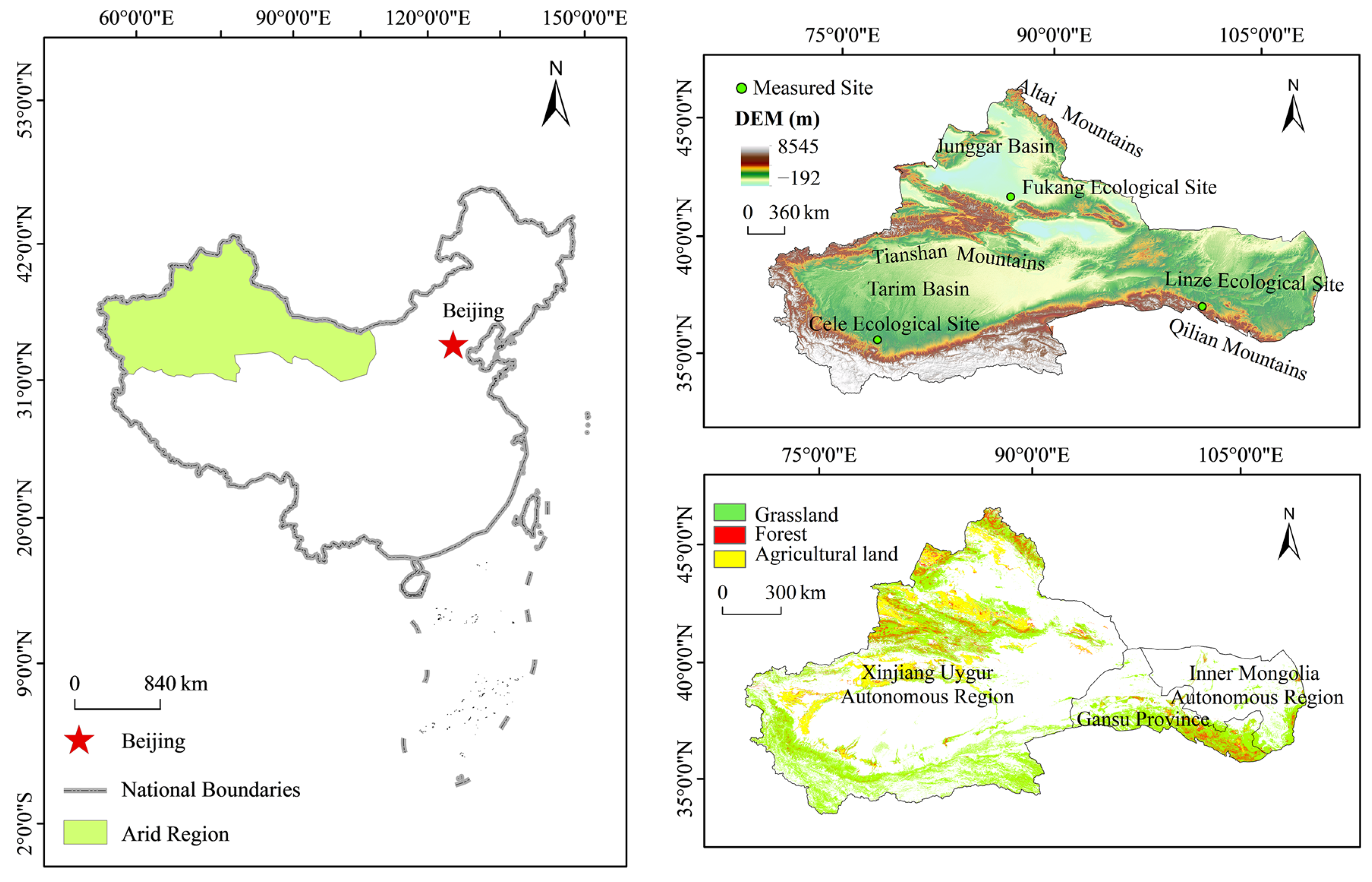
2.1. General Description of Study Area

The arid region of Northwest China is located in the heart of the Eurasian continent at mid-latitudes. Precipitation primarily originates from mountainous areas and glacial meltwater, resulting in an average annual precipitation of <200 mm, characteristic of a continental climate [32]. Geographically, the region (34°44′11″–49°077′24″ N, 73°47′17″–106°43′00″ E) spans from the Pamir Plateau in the west to the Helan Mountains in the east, and from the southern periphery of the Tarim Basin in the south to the Altai Mountains in the north. It encompasses a wide range of altitudes, extending from 192 to 8545 m, covering approximately 2.6 × 10⁶ km², equivalent to 30% of the total land area of China [33]. Within this expanse, there are areas designated for forest land, grassland, cropland, and other land-use types, measuring 6.6 × 10⁴, 5.1 × 10⁴, 4.1 × 10⁴, and 6.7 × 10³ km², respectively [33]. The study area encompasses the Xinjiang Uyghur Autonomous Region, Alashan Plateau of Inner Mongolia, and the area west of the Helan Mountains in the Ningxia Hui Autonomous Region (Figure 1). This area is a vital component of the Central Asian arid zone, ranking among the world’s driest regions at its latitude [34]. Its delicate ecological environment is highly susceptible to global changes [35]. Therefore, it is imperative to investigate the influence of climate change on vegetation growth within this region to preserve ecosystem stability.

2.2. Data Sources and Preprocessing

2.2.1. SIF, EVI, and Gross Primary Production (GPP) Data

Global SIF product (GOSIF) based on Orbiting Carbon Observatory-2 (OCO-2) data was utilised. The spatial and temporal resolution of the dataset from Global Ecology Group’s data repository was 0.05° and 8 d, respectively. (available at http://data.globalecology.unh.edu/data/GOSIF_v2/Annual/, accessed on 6 May 2023), and was created by integrating discrete OCO-2 SIF point clouds with remote sensing data from MODIS and meteorological reanalysis data, spanning from 2001 to 2019.

To ensure the accuracy of our vegetation phenology estimation, we used ArcGIS10.8 software to eliminate data rasters with pixel values of 32,767, representing water bodies, and values of 32,766, indicating year-round snow and ice. This step aimed to mitigate potential interference from water bodies, snow, and ice on our vegetation phenology assessments [36].

For comparative analysis, we obtained EVI and GPP data from the MOD13A1 and MOD17A2H.061 products of MODIS data, accessible through NASA in the United States (https://lpdaac.usgs.gov/, accessed on 5 May 2023). These datasets have temporal resolutions of 16 and 8 days, respectively, with a spatial resolution of 500 m.

To ensure consistency in our analysis, we employed the maximum value synthesis method of ArcGIS10.8 software to harmonise the temporal resolutions of SIF, GPP, and EVI in the study area from 2001 to 2019 at intervals of 16 days. Additionally, we aligned the spatial resolutions of the EVI and GPP datasets with those of SIF, setting them at 0.05° using a downscaling method [37].

2.2.2. Vegetation Type and Meteorological Data

Vegetation type information obtained from the Northwest Institute of Eco-Environment and Resources combined with data from the Second Land Survey (accessible at http://www.nieer.cas.cn/kyfw/kxsj/, accessed on 20 May 2023) were extracted to create a comprehensive vegetation type map of the study area (Figure 1). The prominent vegetation types within the arid zone of Northwest China encompass woodland, grassland, and cropland.

We sourced 1 km month-by-month gridded temperature (TMP) and precipitation (PRE) data for the study area from 2001 to 2019 through the National Earth System Science Data Center (available at http://gre.geodata.cn, accessed on 1 June 2023). This dataset is a fusion of global 0.5° climate data from the Climatic Research Unit, University of East Anglia, and high-resolution climate data from WorldClim (https://worldclim.org, accessed on 2 June 2023), achieved via spatial downscaling methods. Importantly, it has undergone rigorous validation with data obtained from 496 independent meteorological observation sites [38].

To characterise drought conditions within our study area from 2001 to 2019, we employed the standardised precipitation evapotranspiration index (SPEI) with a spatial resolution of 0.5°, which were obtained from the global SPEI database SPEI base v2.7. (https://digital.csic.es/handle/10261/268088, accessed on 2 June 2023). The SPEI amalgamates the strengths of both the Palmer drought severity index (PDSI) and the standardised precipitation index (SPI). SPEI accounts for the processes of moisture and heat balance, offering insights into the extent of the surface water deficit and its accumulation. The China Meteorological Administration (CMA) provides the SPEI drought classification criteria, with SPEI categories as follows: SPEI > −0.5 indicates no drought; −1 < SPEI ≤ −0.5 signifies mild drought; −1.5 < SPEI ≤ −1 denotes moderate drought; −2 < SPEI ≤ −1.5 corresponds to severe drought; and SPEI ≤ −2 represents exceptional drought (https://www.cma.gov.cn/, accessed on 3 June 2023).

2.2.3. MODIS Climate Data and Ground-Based Climate Observations

For the comparative analysis, MODIS phenology product data, MCD12Q2, from the NASA website (https://lpdaac.usgs.gov/, accessed on 4 June 2023) were obtained. These data have a spatial resolution of 500 m. Greenup in the MCD12Q2 product is the period of onset of vegetative growth (SOS_EVI) and dormancy is the period of the end of vegetative growth (EOS_EVI). The MCD12Q2 product utilises a segmented logistic function fitted to the EVI from MODIS as the primary data source. It identifies the extremes of curvature change points in the EVI to determine the initiation, maturity, peak, and conclusion of vegetation growth [37].

MCD12Q2 products spanning 2001 to 2019 were processed by splicing, projecting transformation, and cropping to extract data on the SOS_EVI and EOS_EVI of vegetation within our study area. This allowed calculation of the duration of the vegetation growth period. Climatic parameters were expressed as Julian days, converting the dates of climatic phenomena into the actual number of days from January 1 of the current year (days of the year, doy), thereby creating a time series for each climatic period.

To validate the accuracy of our findings, we sourced ground-based climatic observations from the National Ecological Science Data Center (http://rs.cern.ac.cn/data/meta?id=40177, accessed on 4 June 2023). These observations included climatic data for both herbaceous and woody plants at 21 ecological stations across China, covering the period from 2003 to 2015. To ensure precision, climate observation data from the Fukang, Celle, and Linze stations were selected, as they had recorded data for at least three years and monitored at least eight plant species annually. Additional information about these stations is presented in

Table 1. Sites analysed in the study.

Field Test Site Name	Longitude	Latitude
Linze Station	99°35″	39°04′
Fukang Station	87°55′	44°17′
Cele Station	80°43′	37°00′

.

The Fukang, Celle, and Linze stations are strategically located in desert, grassland, and cropland areas, respectively, and are representative of typical vegetation ecosystems in the northwestern arid zone [36]. For woody plants, the start of the growth period was defined as the leaf-spreading phase, and the end of the period was set as the deciduous phase. For herbaceous plants, the start of the growth season was defined as the average of the greening and flowering periods, while the end of the season was defined as the yellowing period. Since remote sensing technology relies on vegetation greenness data to calculate phenology parameters, there may be some discrepancies with the phenology periods observed at ground stations. To minimise errors, the averages of the different growth seasons of herbaceous and woody plants were defined as the beginning and end of the growing season for each year at the respective station. Data for this site are from the National Ecological Science Data Centre (NESDC) Resource Sharing Service Platform. (http://rs.cern.ac.cn/, accessed on 6 June 2023) [39].

2.3. Vegetation Phenology Extraction

2.3.1. Time Series Reconstruction of SIF Data

SIF time series data are robust against cloud cover and atmospheric scattering. However, random factors and missing values can introduce noise. Therefore, data smoothing is a necessary step. In comparison to the double logistic (DL) and asymmetrical Gaussian (AG) filtering methods, the Savitzky–Golay (S–G) smoothing technique provides smoother and more stable reconstructed curves [40]. This method effectively reduces noise while preserving the nuances and fine details in long time series data [41].

In this study, we employed the S–G filter, which is available in the TIMESAT3.3 software, to reconstruct the SIF data time series from 2001 to 2019 within the study area. This filtering method yielded smoothed curves that can more accurately capture the peaks and valleys within the SIF time series data [20]. The S–G filter utilises an iterative algorithm that relies on convolutional fitting using the least squares method [42]. The process involves specific steps that are detailed below.

In the initial step, for the peaks and valleys evident in the SIF curves before denoising, the left and right segments of the curves are fitted using the S–G function. The local fitting function (f1(t)) is expressed by Equation (1):

$$f1\left(t\right)\equiv f\left(t;a1,a2,b1,\dots ,b5\right)=a1+a2g\left(t;b1,\dots ,b5\right)$$

(1)

where a1 and a2 are linear parameters that ensure a reasonable rate of increase or decrease in the basis function span.

Step two is

$$g\left(t;b1,\dots ,b5\right)=\left\{\begin{array}{c}exp\left[-\left({\frac{1-b_1}{b_2}}^{b_3}\right)\right]\\ exp\left[-\left({\frac{1-b_3}{b_4}}^{b_5}\right)\right]\end{array}\right\}\begin{array}{c}\left(t>b1\right)\\ \\ \left(t>b2\right)\end{array}$$

(2)

where g(t;b1,…,b5) is the S–G function, b1 is the location parameter of the peak or trough of the time variable t, and b2, b3, b4, and b5 are the width and steepness of the left and right halves of the fitted curves, respectively.

The local fitting function model can be used to plot the maximum and minimum values of the SIF curve. The overall fitting function combines the characteristics of the local fitting function [43], which is calculated as

$$f2\left(t\right)=\left\{\begin{array}{c}\alpha \left(t\right)f_L\left(t\right)+\left[1-\alpha \left(t\right)\right]f_C\left(t\right)\\ \beta \left(t\right)f_C\left(t\right)+\left[1-\beta \left(t\right)\right]f_R\left(t\right)\end{array}\right\}\begin{array}{c}(t_L<t<t_C) \\ (t_L<t<t_C) \end{array}$$

(3)

where $f2\left(t\right)$ is the overall fitting function, [t_L, t_C] is the variation interval of the SIF data series, f_L(t), f_C(t), and f_R(t) represent local functions corresponding to the left valley, middle peak, and right valley in the interval [t_L, t_C], respectively, and α(t) and β(t) are the truncation functions located between [0, 1]. The merging of locally fitted functions is a key feature of Gaussian function simulations. This approach increases the flexibility of the fitted functions to simulate more complex time series variations [44].

2.3.2. Dynamic Thresholding

Based on the reconstruction of SIF time series data from 2001 to 2019, the dynamic threshold method was used to extract the vegetation phenology parameters SOS_SIF and EOS_SIF. First, the dynamic threshold of SIF ($SI{F}_{ratio}$) was calculated as

$$SI{F}_{ratio}=\frac{SI{F}_t-SI{F}_{min}}{SI{F}_{max}-SI{F}_{min}}$$

(4)

where SIF_t is the SIF value for a given day in a given year, and SIF_max and SIF_min are the annual maximum and minimum SIF values, respectively, for the time span of the study. SOS_SIF is defined as the doy when the SIF value exceeds the local threshold SIF_ratio. EOS_SIF is defined as the doy when the SIF value is below the local threshold SIF_ratio. Considering the effects of different wavelengths of light on chlorophyll fluorescence, this threshold was set to one-fifth of the difference between SIF_max and SIF_min [45].

2.3.3. Sen and Mann–Kendall Trend Analyses

Sen trend degree was first used to analyse the trend of climate information. Then, Matlab R2021b software was used to test the significance of climate data trends by Mann–Kendall test [46]. The degree of Sen trend is calculated as follows:

$${\beta }_{sif}=median\left(\frac{x_j-x_i}{j-i}\right), 1<i<j<19$$

(5)

where x_j and x_i are the annual mean vegetation phenology doy for the j-th and i-th year image elements, respectively, βsif is the slope of phenology change, β_sif > 0 indicates an upward trend in phenology data, and β_sif < 0 indicates a downward trend in phenology.

The S statistic for the Mann–Kendall trend significance test was calculated as follows:

$$S={{\displaystyle \sum }}_{i=1}^{n-1}{{\displaystyle \sum }}_{j=i+1}^{n}sgn(x_j-x_i)$$

(6)

where the sgn function is a step function that symbolises the difference between x_j and x_i, and is calculated as follows:

$$sgn\left(x_j-x_i\right)=\left\{\begin{array}{c}-1 x_j-x_i<0\\ 0 x_j-x_i=0\\ 1 x_j-x_i>0\end{array}\right\}$$

(7)

The length of the time series data was 19 years, and the statistic S followed a normal distribution. Therefore, the test statistic Z was used to test for trend, and the test was taken at a significant level of α = 0.05 and Z_1−α = Z_0.975 = 1.96 [47]. The Z test statistic was calculated as follows:

$$Z=\left\{\begin{array}{c}\frac{S+1}{\sqrt{VAR\left(S\right)}} S<0\\ 0 S=0\\ \frac{S-1}{\sqrt{VAR\left(S\right)}} S>0\end{array}\right.$$

(8)

where VAR(S) is the variance of the statistic S, calculated as follows:

$$VAR\left(S\right)=\frac{n\left(n-1\right)\left(2n+5\right)-{{\displaystyle \sum }}_{i=1}^m{t}_i\left(t_i-1\right)\left(2t_i+5\right)}{18}$$

(9)

where n is the number of points in the sequence, i is the number of repetitions, m is the number of non-repetitive numbers, and ti is the number of repetitions in the i-th repetitive dataset.

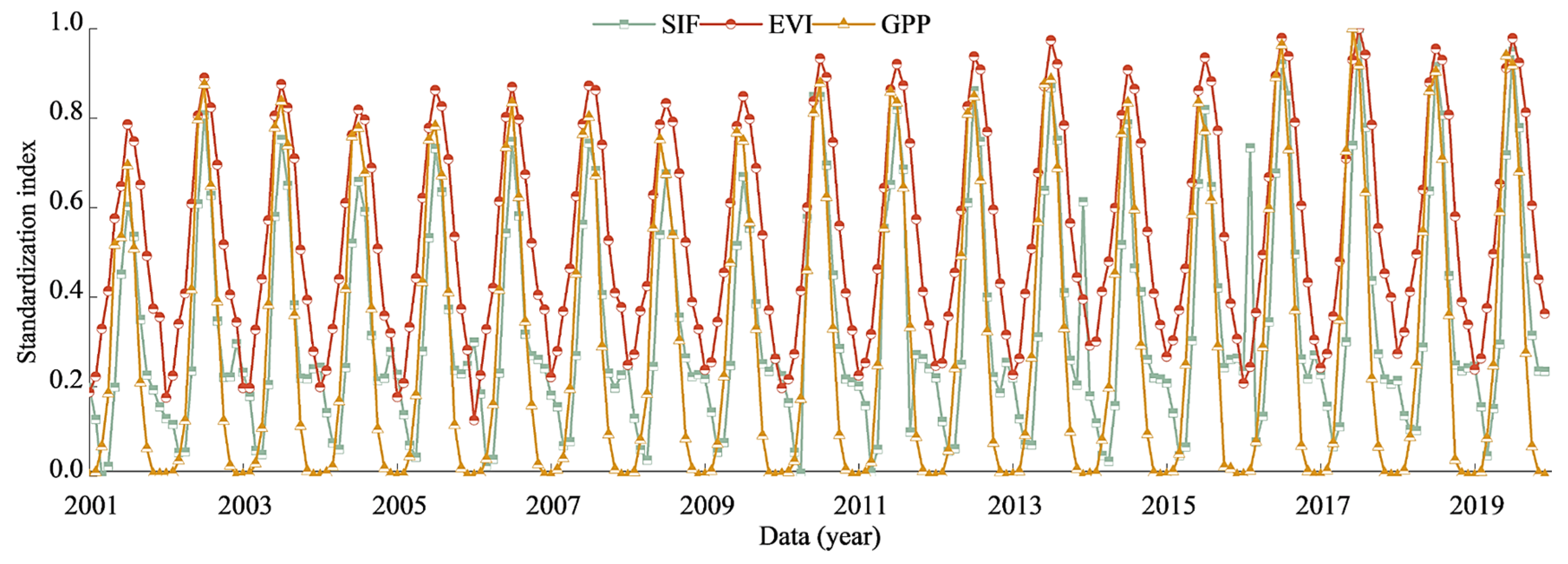
2.4. Standardised Processing

To reduce errors in the evaluation results caused by differences in the nature, scale, and order of magnitude of the evaluation indicators in the multi-indicator evaluation system, it was necessary to standardise the raw data [48,49]. In this study, the minimum-maximum normalization method in ArcGIS10.8 was used to standardize GOSIF, GPP, and EVI data, as follows:

$$y_i=\frac{x_i-min\left(x_j\right)}{\max \left(x_j\right)-min\left(x_j\right)}$$

(10)

where y_i is the result after normalisation of the i-th original data x_i and min(x_j) and max(x_j) represent the minimum and maximum values of the original data, respectively.

2.5. Partial Correlation Analysis

Previous research has demonstrated that partial correlation analysis is an effective approach for examining the connection between vegetation phenological responses and environmental factors in arid regions [50,51]. Specifically, the onset of the phenological period appears to be more responsive to the mean temperature in March and April, precipitation in the preceding November, and the 12-month scale of the standardized precipitation evapotranspiration index (SPEI-12). In contrast, the conclusion of the phenological period is more sensitive to the mean temperature and precipitation in July and August, as well as SPEI-12 [52,53].

In this study, MATLAB R2021b software was used to select the mean temperature in March and April, the precipitation from November of the previous year, and SPEI-12 to analyse their relationships with the onset of the vegetation phenology. Similarly, the mean temperature, precipitation, and SPEI-12 in July and August were chosen as key climatic factors to examine their climate response in relation to the phenological conclusion [52,53].

For the bias correlation analysis between phenological and climatic factors, the other two factors were excluded, and the bias correlation coefficient was computed as follows:

$$R_{xy,z}=\frac{R_{xy}-R_{xz}{r}_{yz}}{\left(1-R_{xz}^2\right)\left(1-R_{yz}^2\right)}$$

(11)

where R_xy,z is the correlation coefficient between x and y after the control variable z, z is the other variable to be excluded, and R_xy, R_xz, and R_yz represent the correlation coefficients of the variables x and y, x and z, and y and z, respectively.

3. Results

3.1. Comparison of GOSIF- and MODIS-Based Phenology

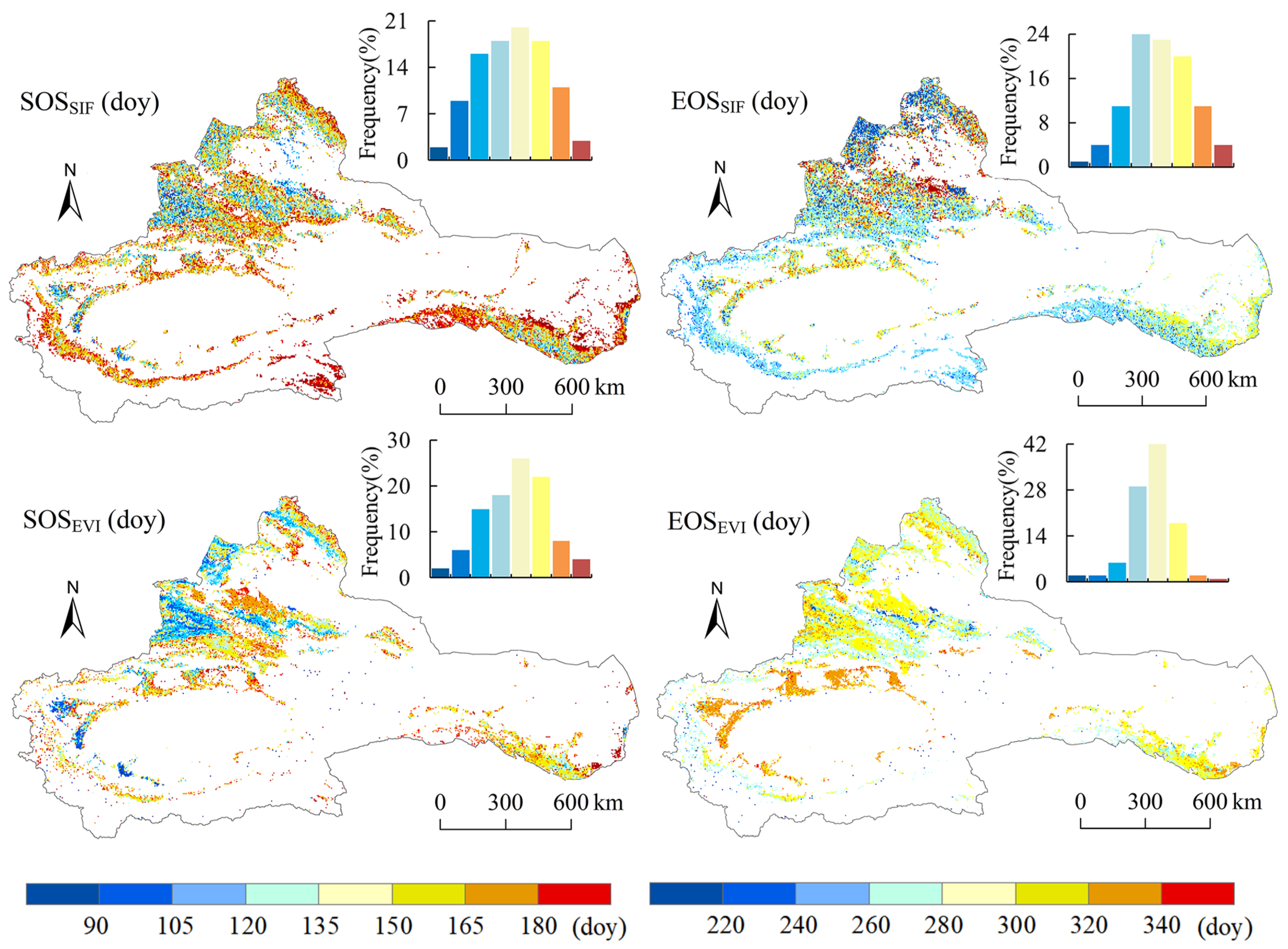
3.1.1. Spatial Characteristics of GOSIF- and MODIS-Based Phenology

The distribution patterns of both the SOS_SIF and EOS_SIF are presented in Figure 2. The multi-year average SOS_SIF exhibited a “late–early–late” pattern from the southeast to the northwest. Within the designated research area, the multi-year average SOS_SIF for vegetation was 149 d, typically falling at the end of April. Vegetation SOS_SIF in this region was predominantly concentrated between 85 and 165 d, from late March to early June. More specifically, in Linze County of Gansu Province and the Junggar Basin area of the Tianshan Mountain Range in Xinjiang, located in the southeast portion of the study area, SOS_SIF was primarily concentrated between 85 and 150 d, from late March to late April. In contrast, in other regions, SOS_SIF was concentrated between 150 and 180 d, from early May to early June. Additionally, the study area exhibited noticeable spatial heterogeneity in vegetation phenology from north to south, with the northern region experiencing a later start to the growing season than the southern region.

SOS_EVI was predominantly concentrated between 70 and 160 d, from mid-March to early June. The multi-year average of SOS_EVI occurred 10 d earlier than that of SOS_SIF, and the spatial distribution patterns of SOS_EVI and SOS_SIF displayed similarities.

The multi-year average EOS_SIF for the study area was 258 d, typically occurring in mid-September. In the southeast and northwest regions, EOS_SIF was mainly concentrated between 260 and 310 d, from mid-September to early November. In contrast, in other regions, EOS_SIF primarily occurred on day 310, in mid- to late-November. The multi-year average EOS_EVI was predominantly concentrated between 260 and 320 d, from late September through late November, and it was on average 25 d later than EOS_SIF. The northern part of the study area saw an earlier conclusion to the growing season in contrast to the southern region. Relative to EOS_EVI, the spatial distribution of EOS_SIF exhibited less heterogeneity and greater uniformity.

Figure 3 illustrates the month-by-month time series data for the mean values of GOSIF, EVI, and GPP in the study area from 2001 to 2019. The curves of these variables display a cyclical single-peak shape, portraying the dynamic attributes of the arid zone’s vegetation growth cycle. The curves of GOSIF, EVI, and GPP all exhibit a cyclical single-peak shape, which corresponds to the typical pattern of vegetation growth cycles in arid regions. These curves exhibit a rapid ascent towards the end of April. The GOSIF curve peaked in mid-June during the growing season, followed by a swift decline. The EVI curve lagged behind the GOSIF curve but eventually coincided in mid-July. The EVI time series curve of MODIS rose earlier than the GPP curve. This finding suggests that the growing season duration derived from vegetation index data exceeded that determined using SIF and GPP.

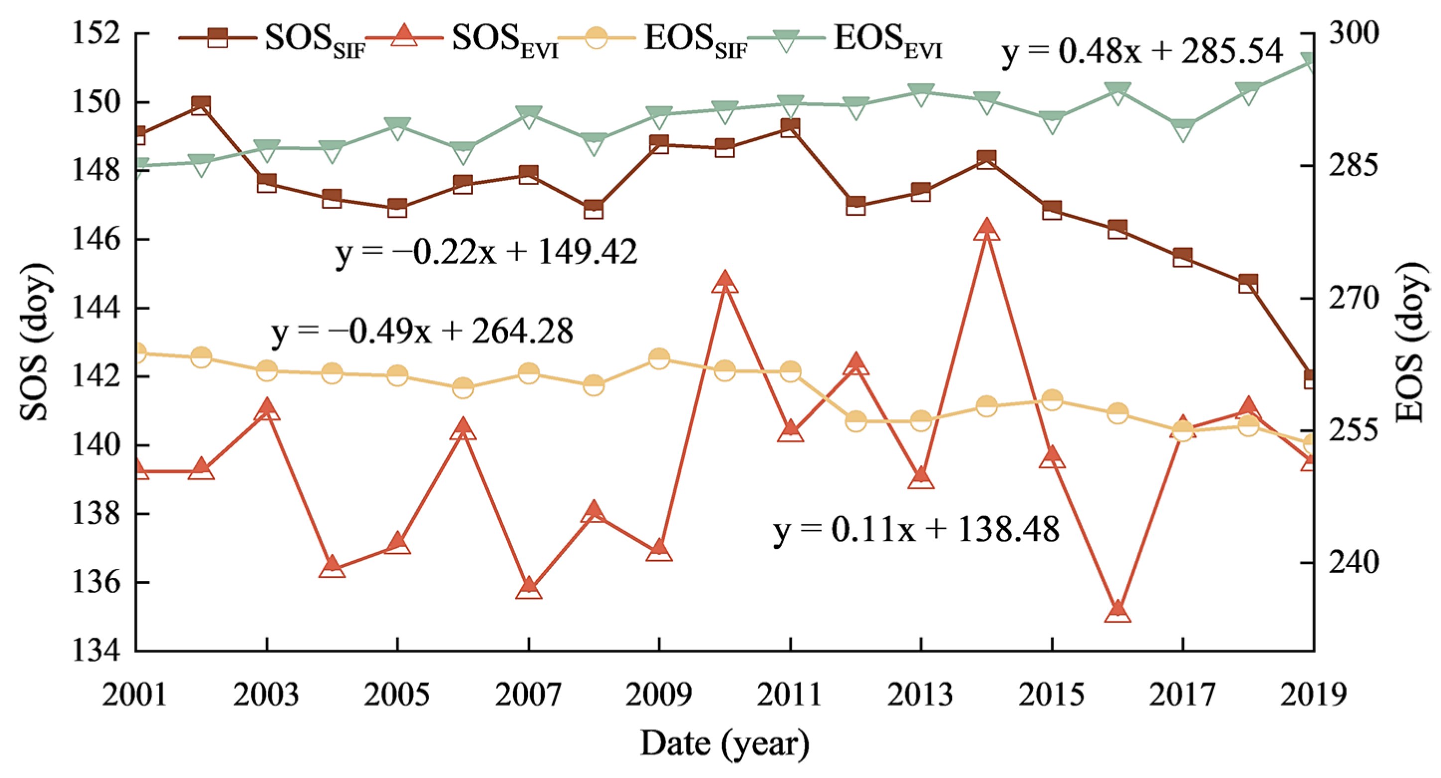
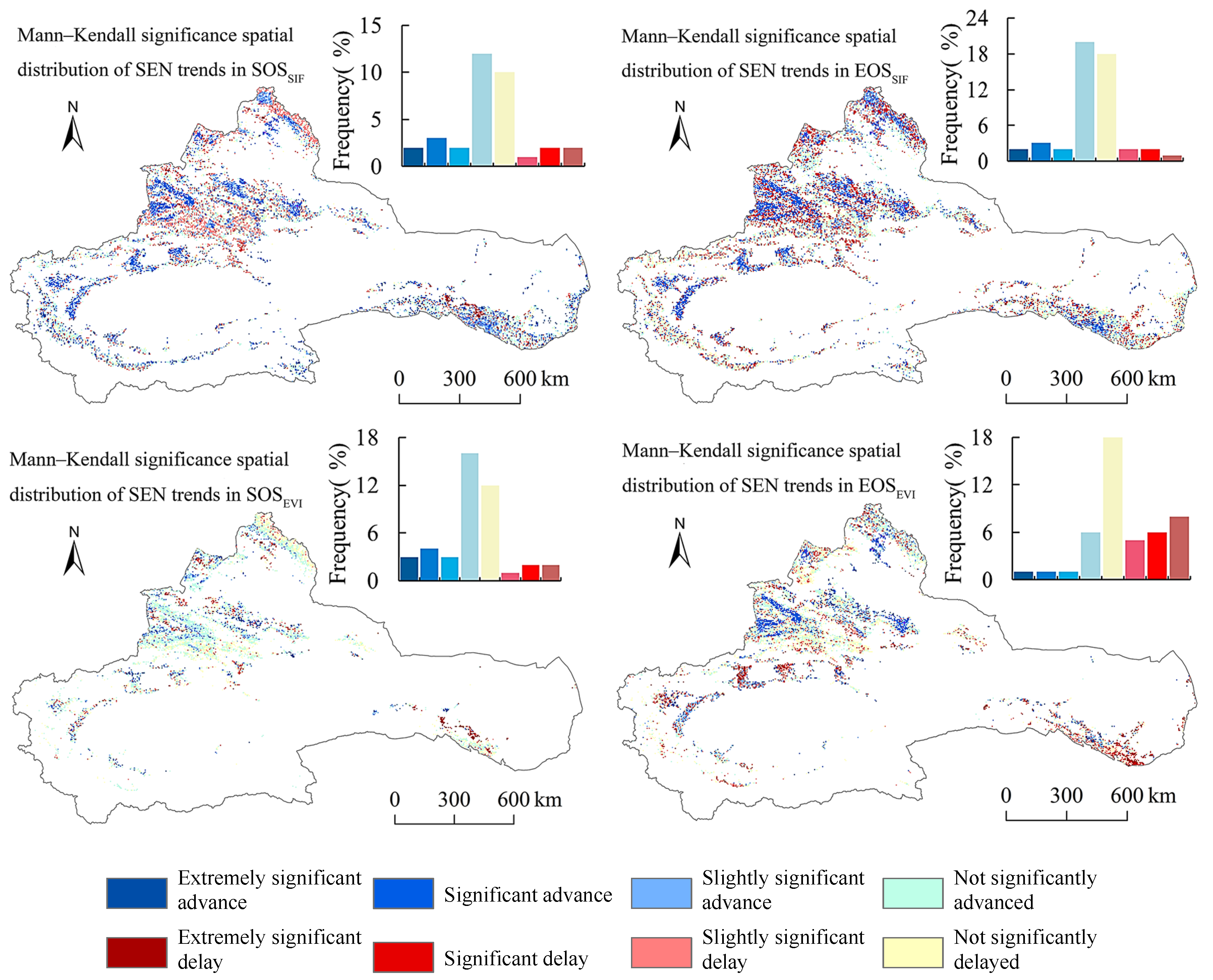
3.1.2. Temporal Trends between GOSIF- and MODIS-Based Phenology

Figure 4 presents the results of Sen trend analysis for vegetation SOS_SIF and EOS_SIF in the study area from 2001 to 2019. Both indicators demonstrated a fluctuating downward trend, with trend degrees of −0.22 and −0.49 d/yr, respectively, signifying an overall advancement in the start and end periods of vegetation growth. On the other hand, the overall SOS_EVI and EOS_EVI in the study area from 2001 to 2019 displayed a fluctuating upward trend. This indicates a delayed trend in the start and end periods of vegetation growth, with delayed trend degrees of 0.11 and 0.48 d/yr, respectively.

Figure 5 presents the MK test results for the trend analysis of vegetation phenology from 2001 to 2019. Over 27.81% of the SOS_SIF image elements displayed an advancing trend, with 9.35% being statistically significant. The significant image elements were primarily located in the Tianshan Mountains and Qilian Mountains. Similarly, more than 33.16% of the EOS_SIF image elements exhibited an advancing trend, with 7.29% being statistically significant. The significant image elements were mainly distributed in the Tian Shan, Altay Shan, Qilian Shan, and Tarim Basins.

In contrast to the SIF climatic trend, 25.79% of the image elements in the vegetation climatic SOS_EVI showed a delayed trend, with 6.96% being statistically significant. For EOS_EVI, 46.36% of the image elements displayed delayed trends, with 18.93% being statistically significant. The significant image elements were primarily situated in the Qilian Mountains and Altai Mountains.

3.2. Sensitivity of Vegetation Phenology to Environmental Factors

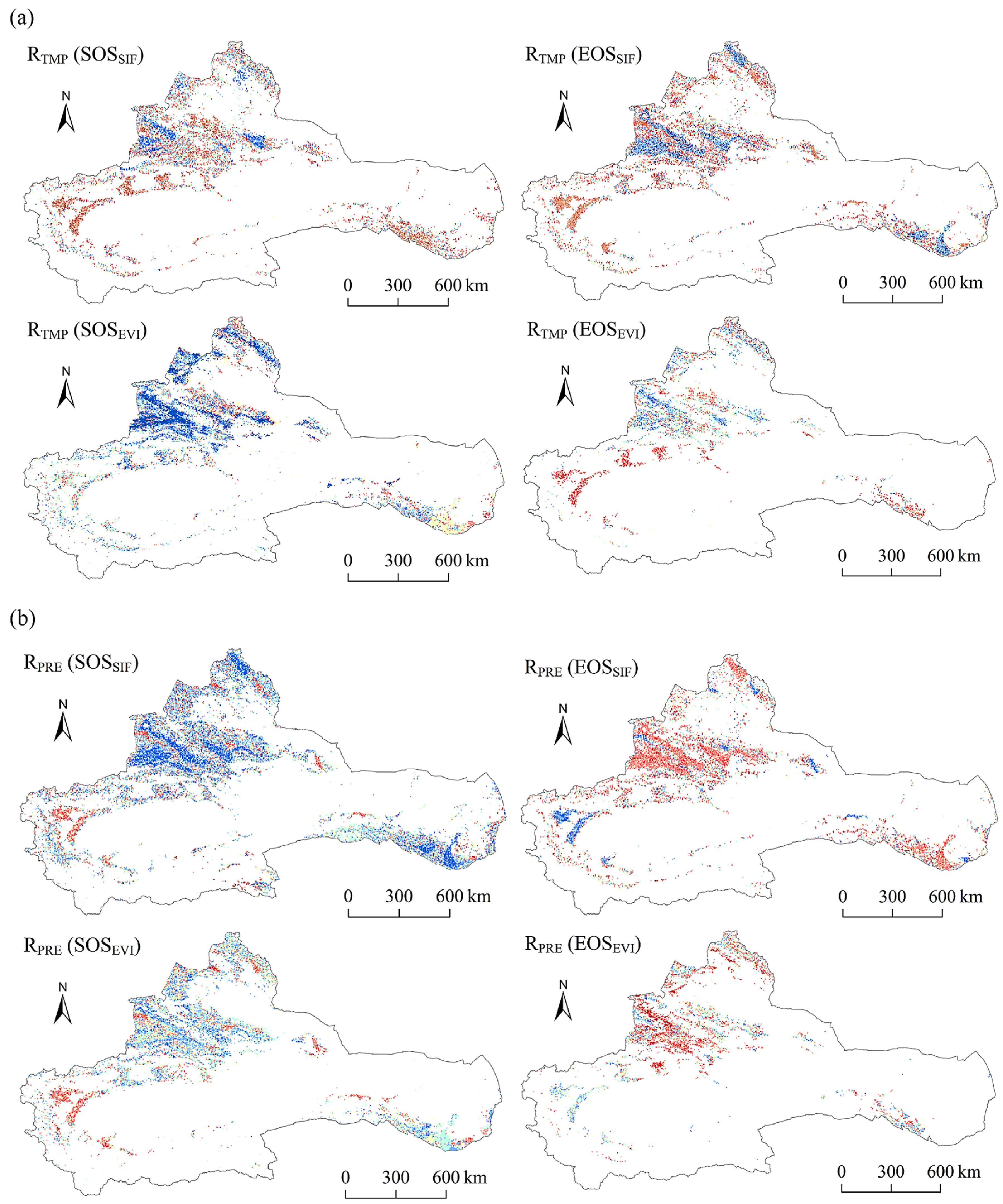
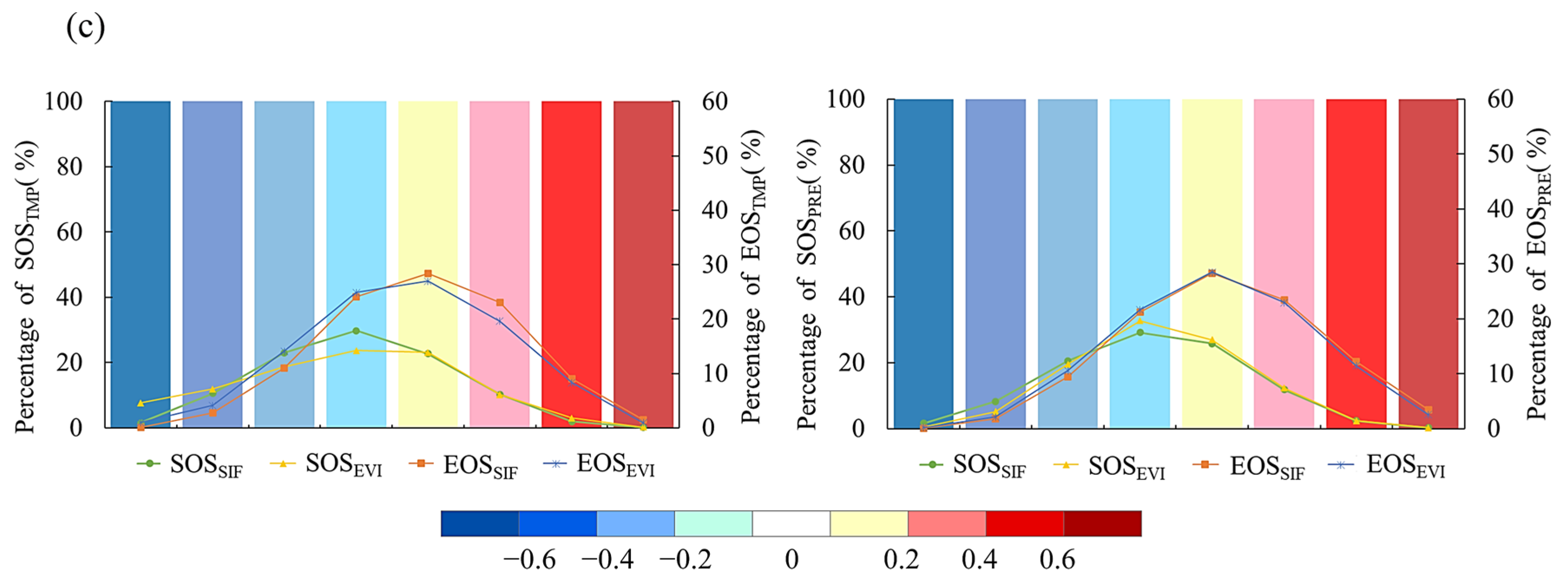
3.2.1. Sensitivity of GOSIF- and MODIS-Based Phenology to Hydrothermal Changes

The results of the bias correlation analysis between the mean temperature in March–April and the precipitation in November of the previous year with corresponding climatic parameters for the same years revealed several insights (Figure 6). The average annual mean temperature from March to April exhibited a negative correlation with both SOS_SIF and SOS_EVI. In other words, as the temperature increased, the beginning of the growing season advanced. Specifically, 64.99% of SOS_SIF pixels and 62.86% of SOS_EVI pixels in the study area were negatively correlated with temperature, with 7.10% and 5.29% of pixels showing a significant negative correlation. These significant correlations were primarily observed within the Tianshan region’s northern and southern slopes, northern Altai, and western Qilian Mountains. Additionally, the average precipitation in November of the previous year showed a negative correlation with both SOS_SIF and SOS_EVI in 59.65% and 58.03% of the pixels, respectively. These negative correlations were primarily concentrated in the Tarim Basin, the eastern Altai Mountains, and the western Qilian Mountains.

The impact of climatic factors on the termination of vegetation growth in the study area is more intricate. As indicated in Figure 6, 61.97% and 55.82% of the image elements of EOS_SIF and EOS_EVI exhibited positive correlations with the multi-year mean temperature in July and August. Additionally, 5.29% and 7.16% of the image elements had statistically significant positive correlations (Figure 7). These findings suggest that an increase in temperature leads to a delay at the end of the vegetation growth period. EOS_SIF and EOS_EVI also displayed positive correlations with 67.42% and 65.41% of the image elements with multi-year average July and August precipitation, respectively. Moreover, 7.79% and 9.11% of the image elements exhibited significant positive correlations. These findings suggest that greater precipitation is linked to a prolonged vegetation growth season. The significant image elements were primarily located in the Altay, Tianshan, and western Qilian Mountains.

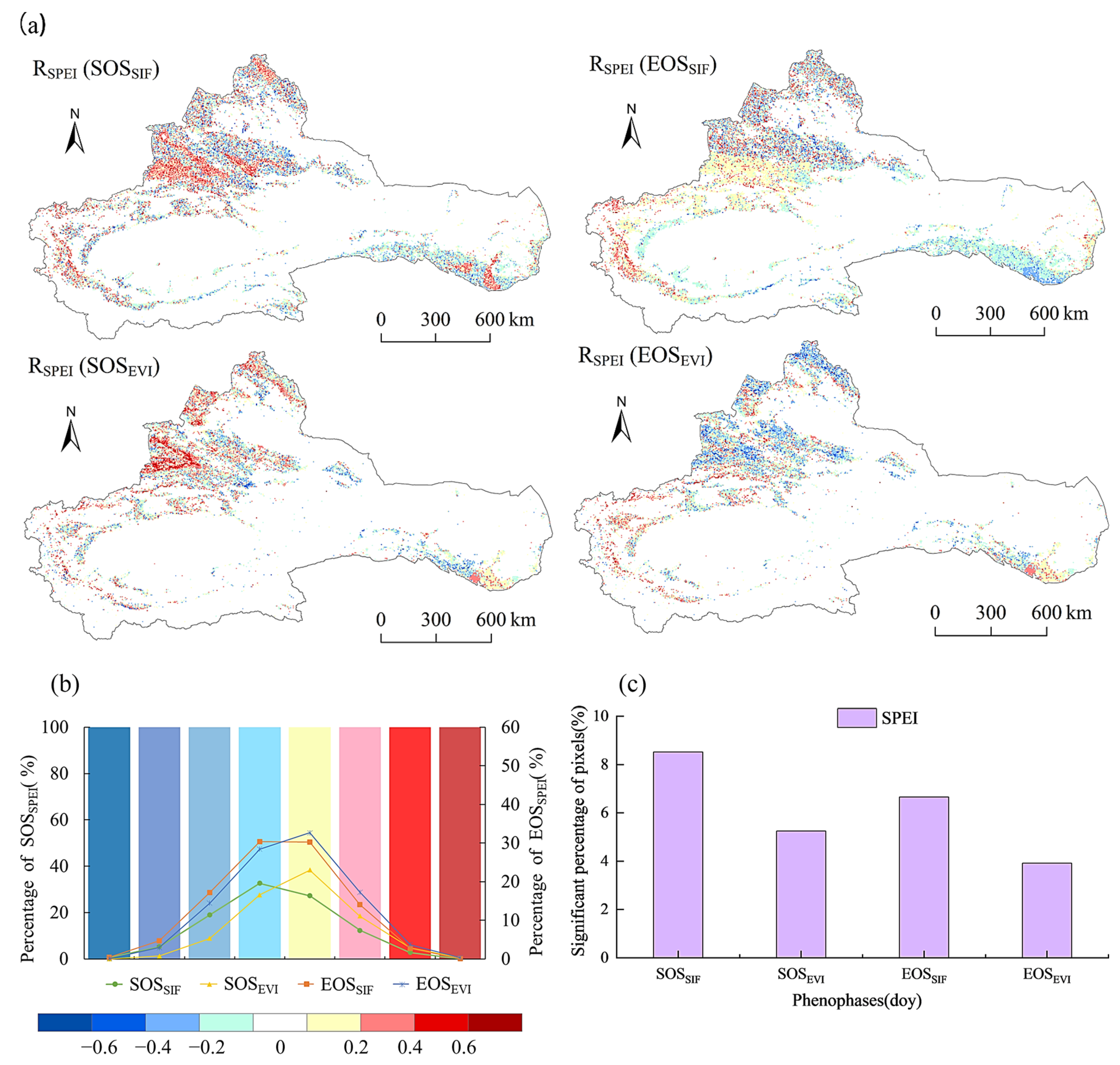
3.2.2. Sensitivity of GOSIF- and MODIS-Based Phenology to SPEI

When precipitation and temperature were constant, it was observed that in the study area, the proportion of image elements with a negative correlation between SOS_SIF and SOS_EVI and the annual mean SPEI was 59.65% and 58.03%, respectively (Figure 8). This means that, overall, with a decrease in the degree of drought, the beginning of the vegetation growth period has advanced. Of these correlations, 8.52% and 5.25% of the pixels displayed statistically significant negative correlations, primarily located in the eastern Altai Mountains, western Tianshan Mountains, Tarim Basin, and western Qilian Mountains.

Conversely, the proportions of EOS_SIF and EOS_EVI were positively correlated with the annual average drought degrees of 67.42% and 65.41%, respectively. In general, these findings suggest that the end of the vegetation growth period was delayed by a decrease in drought severity. Statistically significant positive correlations were observed in 6.66% and 3.92% of the pixels, mainly found on the southern slopes of the western Altai Mountains, Tianshan Mountains, and the Tarim Basin.

In summary, in comparison to SOS_EVI and EOS_EVI, there were more image elements with significant correlations between vegetation SOS_SIF and EOS_SIF and SPEI in the study area. This indicates that vegetation SOS_SIF and EOS_SIF in arid regions exhibited greater sensitivity to SPEI.

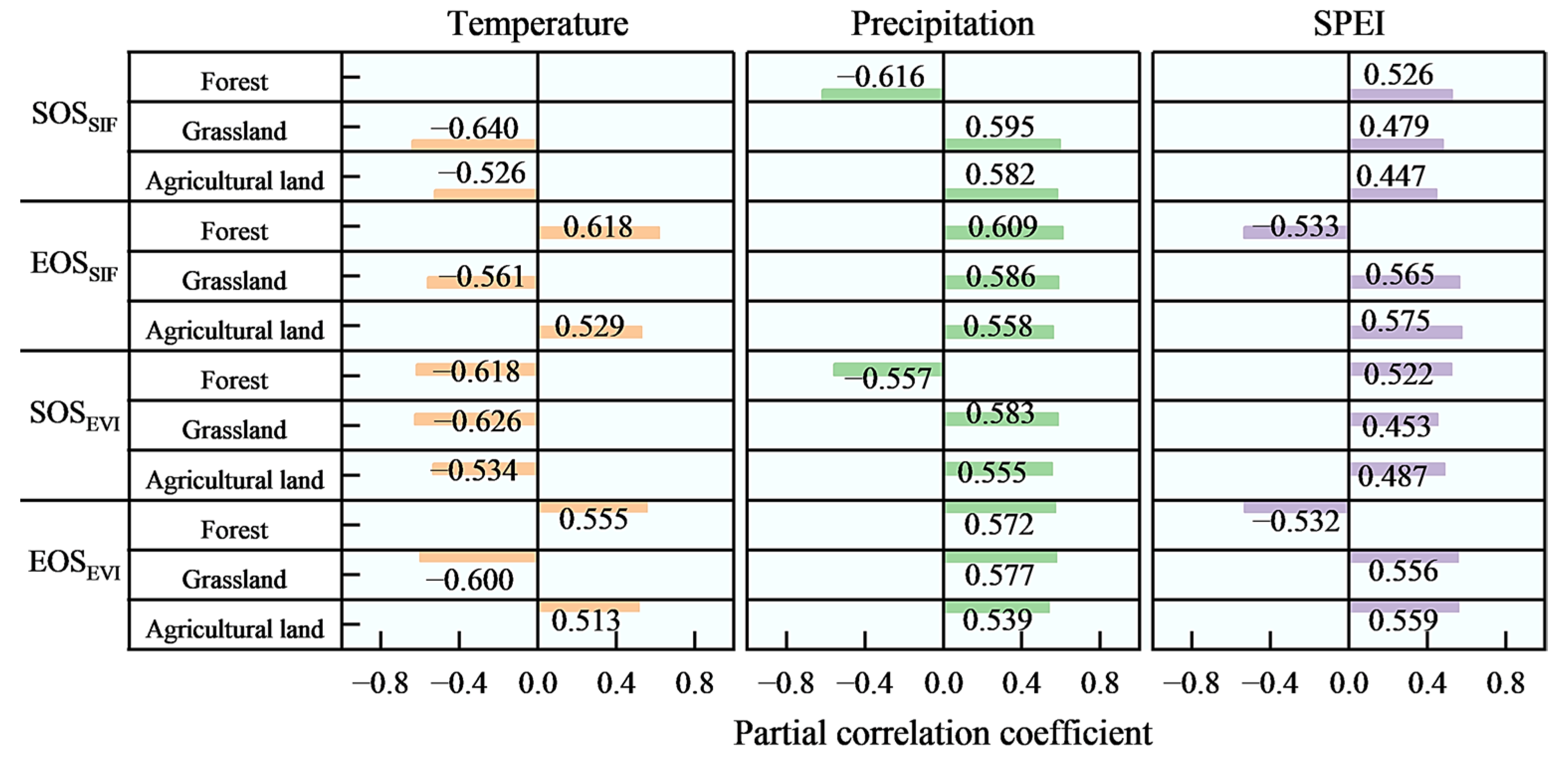
3.2.3. Phenological Response to Environmental Factors across Diverse Vegetation Types

As depicted in Figure 9, the climatic responses of the three primary vegetation types (forest, grassland, and cropland) in the study area to temperature, precipitation, and SPEI extracted from GOSIF and MODIS data were consistent across the study area. However, GOSIF-extracted vegetation demonstrated greater sensitivity to climate in comparison to MODIS-extracted vegetation.

For GOSIF-extracted forest growth, the bias correlation coefficients with climate factors were higher than those for MODIS-extracted forest growth. The difference between the bias correlation coefficients of GOSIF-extracted forest growth and climate, compared to MODIS forest growth and temperature, was most pronounced, with a difference of 0.063. This indicates that GOSIF-extracted forest growth was highly sensitive to all three climatic indicators.

In the case of croplands, the bias correlation coefficients of SOS_EVI with temperature and SPEI were higher than those of SOS_SIF. Similarly, the bias correlation coefficient of EOS_EVI with grassland temperature was greater than that of EOS_SIF, with a difference of 0.016. Furthermore, the bias correlation coefficient of SOS_SIF with cropland precipitation was larger than that of SOS_EVI, with a difference of 0.027. This means that the SOS_SIF of the croplands was more sensitive to precipitation than the SOS_EVI.

3.3. Verification of Phenological Results

As depicted in Figure 10, Field-measured climate data from the Linze, Fukang, and Celle stations was used to validate and compare the vegetation estimated by the GOSIF and MODIS climate products. The validation results of the three stations in Figure 10 show that there was an overestimation of SOS_SIF and an underestimation of SOS_EVI compared with the observed data. However, SOS_SIF was closer to the measured data. The EOS_SIF and EOS_EVI curves are distributed on both sides of the measured data curves. The SOS_SIF curves show a later time than that of SOS_EVI, while the EOS_SIF curves show a later time than that of EOS_EVI.

4. Discussion

4.1. Temporal and Spatial Differences in GOSIF- and EVI-Based Phenology

This discrepancy can be attributed to the fact that the response to precipitation primarily dominates during the growth-opening period of croplands in the study area [54]. In contrast, the growth-ending period of grassland is influenced by a combination of various climatic factors, including precipitation and SPEI, and the response to precipitation is more sensitive during the growth-ending period of grassland [54,55]. Therefore, vegetation phenology data extracted using GOSIF can enhance the accuracy of phenological responses to climate change.

Figure 3 is consistent with prior research findings [56,57]. As SIF is the fluorescence signal emitted by plant leaves during photosynthesis, EVI is mainly used to reflect factors that include vegetation cover. This timing difference can be attributed to the fact that in the early stages of the growing season, the ecosystem is still in the carbon source stage, with plants beginning to respire before the leaf spreading stage. Photosynthesis of vegetation leaves occurs later than ecosystem respiration, causing the extraction of the beginning of the growing season based on vegetation index data to be earlier than that based on GOSIF data [58,59]. Similarly, at the end of the growing season, the degradation of chlorophyll in vegetation leaves is a slower process than the decline in photosynthesis, resulting in a lag in the extraction of the end of the growing season based on EVI data compared to that based on GPP data [60].

Figure 4 depicts the spatial trends of the mean values of SOS_SIF and SOS_EVI of the multi-year vegetation. The spatial distribution was characterised by a gradual advance and then a delay from southeast to northwest. The spatial trends of vegetation EOS_SIF and EOS_EVI were mainly characterised by advancement, whereas SOS_SIF was delayed. The reason for the discrepancies in fall phenology could be attributed to the degradation of chlorophyll in leaves and the appearance of other pigments, such as carotenoids and anthocyanins, leading to changes in the reflectance of vegetation in visible and near-infrared spectra and impacting the accuracy of EVI-based fall phenology, whereas SIF-extracted fall phenology effectively avoids such spectral interference [5,45].

In addition, some studies have shown that the vegetation phenology reflected by SIF is more consistent with the wind and wave areas of the flux tower [61]. The SOS_SIF curves are shown earlier than those in EOS_EVI. This difference may be because photosynthesis starts after plant leaf unfolding and stops before leaf senescence. The similarities and differences between the phenological periods extracted from GOSIF and MODIS EVI contribute to the understanding of the mechanisms that drive ecosystem phenological periods and their carbon cycling [28]. In addition, the differences between EOS_SIF and EOS_EVI indicate the complexity of the end period of vegetation growth (i.e., fall phenology). Previous findings have shown that autumn warming leads to increased carbon loss due to enhanced respiration [62]. As shown in Figure 10, the fall phenology extracted based on GOSIF ended earlier than that based on MODIS EVI. This is likely because vegetation may have stopped absorbing photosynthetic carbon in late fall but still maintained the greenness of the leaves [63]. This further elucidates why increased autumn warming could result in a net loss of ecosystem carbon. These findings provide important insights into vegetation phenology and reveal the influence of environmental factors on phenological periods and the mechanisms by which they affect carbon cycling. However, further studies are needed to validate these observations and probe the response mechanisms of SIF and EVI to phenology under different environmental conditions.

4.2. Uncertainty Analysis

This study considered two main aspects of uncertainty. First, there is a scale effect in remote sensing of vegetation phenology. The MODIS phenology product possesses a 500 m spatial resolution, and GOSIF has a spatial resolution of 0.05° × 0.05°. Regional differences in phenology estimated from remote sensing data with different spatial resolutions have been analysed [64]. In terms of temporal resolution, the reliability of sky-scale remote sensing data is low because of the influence of the atmosphere and sensors. Furthermore, reconstruction methods for time series remote sensing data can introduce errors in the estimation of phenology. The S–G filtering method used in this study has a better effect on noise removal [65,66]. However, owing to the inability of the time series data curves of GOSIF and MODIS EVI to completely overlap, the growth cycle is not completely symmetrical, resulting in an algorithm for extracting the beginning of the vegetation growth period that is unable to extract the end of the growth period well [41].

Furthermore, while SIF is related to photosynthetic activity, photosynthesis in plants is a multifaceted physiological process affected by diverse environmental factors. Thus, accurately interpreting plant physiological states from SIF data may require the consideration of multiple factors to better understand the underlying processes [67]. This paper compares the applicability of SIF and EVI in estimating phenology in arid zones and their sensitivity to climate, so as to find the most suitable remote sensing index for estimating vegetation phenology in arid zones, and also provides a theoretical basis for responding to climate change by vegetation phenology in arid zones around the world. However, the accuracy of the results in this study was affected by the spatial resolution of the SIF and EVI. Therefore, the accuracy can be further improved using the following two methods. The first method integrates many types of new high-resolution remote sensing indices to improve the climate monitoring ability of SIF, such as VPP, PPI, and NDGI. Secondly, it is also possible to combine meteorological factors to calibrate the critical period of phenology for different vegetation types based on existing remote sensing estimations of phenology to improve the precision of phenology monitoring in SIF [68,69].

5. Conclusions

In this study, a comparative analysis was performed to examine how climatic factors affected vegetation phenology in the arid region of Northwest China from 2001 to 2019, utilising data from GOSIF and MODIS EVI. The key findings of the study are as follows:

(1)

The overall SOS_SIF of the perennial vegetation in the study area was later than the SOS_EVI, whereas the overall EOS_SIF was earlier than the EOS_EVI. Validation results indicated that SIF-based phenology estimations were more consistent with ground-truth data than those derived from MODIS EVI. The beginning and ending phases of vegetation phenology growth exhibited similar spatial patterns, but the ending phase showed more significant spatial heterogeneity compared to the beginning phase. The spatial distributions of the change trends of SOS_SIF and SOS_EVI were relatively consistent. However, the spatial trends of EOS_SIF and EOS_EVI varied; EOS_SIF mainly exhibited a trend of advancement, while SOS_SIF exhibited a trend of delay in SOS_SIF.

(2)

The vegetation phenology extracted from GOSIF was more sensitive to temperature, precipitation, and SPEI compared to that derived from MODIS EVI. Temperature, precipitation, and SPEI were negatively correlated with the initiation of the vegetation growth period, while temperature was negatively correlated with the end of the growth period. Precipitation and SPEI were positively correlated with the end of the growth period. In terms of spatial distribution, vegetation phenology showed a higher level of sensitivity to climate factors in specific regions, including the Altay Mountains, Tianshan Mountains, western Qilian Mountains, and Tarim Basin.

(3)

The vegetation phenology of forests, grasslands, and croplands extracted using GOSIF exhibited higher sensitivity to temperature, precipitation, and SPEI compared to those derived from MODIS EVI. Specifically, croplands exhibited greater sensitivity to precipitation, and the fall phenology of grasslands was primarily influenced by precipitation and SPEI. These findings indicate that employing SIF extraction to investigate the response of vegetation phenology to climate change in arid regions can yield more scientifically meaningful insights.

In summary, the study demonstrates the effectiveness of using SIF data (GOSIF) for assessing vegetation phenology and how it reacts to climatic factors in arid regions, highlighting its advantages in terms of sensitivity and accuracy compared to MODIS EVI. These findings emphasise the significance of considering SIF extraction when conducting future research on vegetation phenology in arid zones.

References

1. Piao, S.; Liu, Q.; Chen, A.; Janssens, I.A.; Fu, Y.; Dai, J.; Liu, L.; Lian, X.; Shen, M.; Zhu, X. Plant phenology and global climate change: Current progresses and challenges. Glob. Chang. Biol. 2019, 25, 1922–1940. [Google Scholar] [CrossRef]
2. Thompson, J.A.; Paull, D.J. Assessing spatial and temporal patterns in land surface phenology for the Australian Alps (2000–2014). Remote Sens. Environ. 2017, 199, 1–13. [Google Scholar] [CrossRef]
3. Kariyeva, J.; Van Leeuwen, W. Environmental drivers of NDVI-based vegetation phenology in Central Asia. Remote Sens. 2011, 3, 203–246. [Google Scholar] [CrossRef]
4. Porter, J.R.; Challinor, A.J.; Henriksen, C.B.; Howden, S.M.; Martre, P.; Smith, P. Leaf onset in the northern hemisphere triggered by daytime temperature. Nat. Commun. 2019, 6, 6911. [Google Scholar]
5. Liu, X.; Liu, L.; Hu, J.; Guo, J.; Du, S. Improving the potential of red SIF for estimating GPP by downscaling from the canopy level to the photosystem level. Agric. For. Meteorol. 2020, 281, 107846. [Google Scholar] [CrossRef]
6. Yu, H.; Luedeling, E.; Xu, J. Winter and spring warming result in delayed spring phenology on the Tibetan Plateau. Proc. Natl Acad. Sci. USA 2010, 107, 22151–22156. [Google Scholar] [CrossRef] [PubMed]
7. Araghi, A.; Martinez, C.J.; Adamowski, J.; Olesen, J.E. Associations between large-scale climate oscillations and land surface phenology in Iran. Agric. For. Meteorol. 2019, 278, 107682. [Google Scholar] [CrossRef]
8. Zhang, X.; Friedl, M.A.; Schaaf, C.B. Sensitivity of vegetation phenology detection to the temporal resolution of satellite data. Int. J. Remote Sens. 2009, 30, 2061–2074. [Google Scholar] [CrossRef]
9. Shen, X.; Liu, B.; Henderson, M.; Wang, L.; Wu, Z.; Wu, H.; Jiang, M.; Lu, X. Asymmetric effects of daytime and nighttime warming on spring phenology in the temperate grasslands of China. Agric. For. Meteorol. 2018, 259, 240–249. [Google Scholar] [CrossRef]
10. Xue, J.; Su, B. Significant remote sensing vegetation indices: A review of developments and applications. J. Sens. 2017, 2017, 1353691. [Google Scholar] [CrossRef]
11. Cui, L.; Shi, J. Evaluation and comparison of growing season metrics in arid and semi-arid areas of northern China under climate change. Ecol. Indic. 2021, 121, 107055. [Google Scholar] [CrossRef]
12. Wang, Y.; Chen, Y.; Li, P.; Zhan, Y.; Zou, R.; Yuan, B.; Zhou, X. Effect of Snow Cover on Detecting Spring Phenology from Satellite-Derived Vegetation Indices in Alpine Grasslands. Remote Sens. 2022, 14, 5725. [Google Scholar] [CrossRef]
13. Zhu, G.; Wang, X.; Xiao, J.; Zhang, K.; Wang, Y.; He, H.; Li, W.; Chen, H. Daytime and nighttime warming has no opposite effects on vegetation phenology and productivity in the northern hemisphere. Sci. Total Environ. 2022, 822, 153386. [Google Scholar] [CrossRef] [PubMed]
14. Leng, S.; Huete, A.; Cleverly, J.; Yu, Q.; Zhang, R.; Wang, Q. Spatiotemporal variations of dryland vegetation phenology revealed by satellite-observed fluorescence and greenness across the North Australian Tropical Transect. Remote Sens. 2022, 14, 2985. [Google Scholar] [CrossRef]
15. Miao, L.; Müller, D.; Cui, X.; Ma, M. Changes in vegetation phenology on the Mongolian Plateau and their climatic determinants. PLoS ONE 2017, 12, e0190313. [Google Scholar] [CrossRef] [PubMed]
16. Fang, J.; Li, X.; Xiao, J.; Yan, X.; Li, B.; Liu, F. Vegetation photosynthetic phenology dataset in northern terrestrial ecosystems. Sci. Data 2023, 10, 300. [Google Scholar] [CrossRef] [PubMed]
17. Zhang, Z.; Guanter, L.; Porcar-Castell, A.; Rossini, M.; Pacheco-Labrador, J.; Zhang, Y. Global modeling diurnal gross primary production from OCO-3 solar-induced chlorophyll fluorescence. Remote Sens. Environ. 2023, 285, 113383. [Google Scholar] [CrossRef]
18. Yang, X.; Tang, J.W.; Mustard, J.F.; Lee, J.E.; Rossini, M.; Joiner, J.; Munger, J.W.; Kornfeld, A.; Richardson, A.D. Solar-induced chlorophyll fluorescence that correlates with canopy photosynthesis on diurnal and seasonal scales in a temperate deciduous forest. Geophys. Res. Lett. 2015, 42, 2977–2987. [Google Scholar] [CrossRef]
19. Lu, X.L.; Liu, Z.Q.; Zhou, Y.Y.; Liu, Y.L.; An, S.Q.; Tang, J.W. Comparison of phenology estimated from reflectance-based indices and solar-induced chlorophyll fluorescence (SIF) observations in a temperate forest using GPP-based phenology as the standard. Remote Sens. 2018, 10, 932. [Google Scholar] [CrossRef]
20. Meng, F.; Huang, L.; Chen, A.; Zhang, Y.; Piao, S. Spring and autumn phenology across the Tibetan Plateau inferred from normalized difference vegetation index and solar-induced chlorophyll fluorescence. Big Earth Data 2021, 5, 182–200. [Google Scholar] [CrossRef]
21. Li, C.; Peng, L.; Zhou, M.; Wei, Y.; Liu, L.; Li, L.; Liu, Y.; Dou, T.; Chen, J.; Wu, X. SIF-Based GPP Is a Useful Index for Assessing Impacts of Drought on Vegetation: An Example of a Mega-Drought in Yunnan Province, China. Remote Sens. 2022, 14, 1509. [Google Scholar] [CrossRef]
22. Chen, A.; Meng, F.; Mao, J.; Ricciuto, D.; Knapp, A.K. Photosynthesis phenology, as defined by solar-induced chlorophyll fluorescence, is overestimated by vegetation indices in the extratropical Northern Hemisphere. Agric. For. Meteorol. 2022, 323, 109027. [Google Scholar] [CrossRef]
23. Sun, Y.; Frankenberg, C.; Jung, M.; Joiner, J.; Guanter, L.; Köhler, P.; Magney, T. Overview of Solar-Induced chlorophyll Fluorescence (SIF) from the Orbiting Carbon Observatory-2: Retrieval, cross-mission comparison, and global monitoring for GPP. Remote Sens. Environ. 2018, 209, 808–823. [Google Scholar] [CrossRef]
24. Xin, Q.; Li, J.; Li, Z.; Li, Y.; Zhou, X. Evaluations and comparisons of rule-based and machine-learning-based methods to retrieve satellite-based vegetation phenology using MODIS and USA National Phenology Network data. Int. J. Appl. Earth Obs. 2020, 93, 102189. [Google Scholar] [CrossRef]
25. Rad, A.M.; Ashourloo, D.; Shahrabi, H.S.; Nematollahi, H. Developing an automatic phenology-based algorithm for rice detection using sentinel-2 time-series data. IEEE J. Sel. Top. Appl. Earth Obs. Remote Sens. 2019, 12, 1471–1481. [Google Scholar] [CrossRef]
26. Bartold, M.; Kluczek, M. A Machine Learning Approach for Mapping Chlorophyll Fluorescence at Inland Wetlands. Remote Sens. 2023, 15, 2392. [Google Scholar] [CrossRef]
27. Joiner, J.; Yoshida, Y.; Vasilkov, A.P.; Schaefer, K.; Jung, M.; Guanter, L.; Zhang, Y.; Garrity, S.; Middleton, E.M.; Huemmrich, K.F.; et al. The seasonal cycle of satellite chlorophyll fluorescence observations and its relationship to vegetation phenology and ecosystem atmosphere carbon exchange. Remote Sens. Environ. 2014, 152, 375–391. [Google Scholar] [CrossRef]
28. Walther, S.; Voigt, M.; Thum, T.; Gonsamo, A.; Zhang, Y.G.; Köhler, P.; Jung, M.; Varlagin, A.; Guanter, L. Satellite chlorophyll fluorescence measurements reveal large-scale decoupling of photosynthesis and greenness dynamics in boreal evergreen forests. Glob. Chang. Biol. 2016, 22, 2979–2996. [Google Scholar] [CrossRef]
29. Lu, X.C.; Cheng, X.; Li, X.L.; Chen, J.Q.; Sun, M.M.; Ji, M.; He, H.; Wang, S.Y.; Li, S.; Tang, J.W. Seasonal patterns of canopy photosynthesis captured by remotely sensed sun-induced fluorescence and vegetation indexes in mid-to-high latitude forests: A cross-platform comparison. Sci. Total Environ. 2018, 644, 439–451. [Google Scholar] [CrossRef]
30. Zhu, W.; Pan, Y.; He, H.; Yu, D.; Hu, H. Simulation of maximum light use efficiency for some typical vegetation types in China. Chin. Sci. Bull. 2006, 51, 457–463. [Google Scholar] [CrossRef]
31. Shen, X.; Liu, B.; Xue, Z.; Jiang, M.; Lu, X.; Zhang, Q. Spatiotemporal variation in vegetation spring phenology and its response to climate change in freshwater marshes of Northeast China. Sci. Total Environ. 2019, 666, 1169–1177. [Google Scholar] [CrossRef]
32. Yao, J.; Chen, Y.; Guan, X.; Zhao, Y.; Chen, J.; Mao, W. Recent climate and hydrological changes in a mountain–basin system in Xinjiang, China. Earth-Sci. Rev. 2022, 226, 103957. [Google Scholar] [CrossRef]
33. Huo, Z.; Dai, X.; Feng, S.; Kang, S.; Huang, G. Effect of climate change on reference evapotranspiration and aridity index in arid region of China. J. Hydrol. 2013, 492, 24–34. [Google Scholar] [CrossRef]
34. Yang, H.; Mu, S.; Li, J. Effects of ecological restoration projects on land use and land cover change and its influences on territorial NPP in Xinjiang, China. Catena 2014, 115, 85–95. [Google Scholar] [CrossRef]
35. Chen, D.; Liu, W.; Huang, F.; Li, Q.; Uchenna-Ochege, F.; Li, L. Spatial-temporal characteristics and influencing factors of relative humidity in arid region of Northwest China during 1966–2017. J. Arid Land 2020, 12, 397–412. [Google Scholar] [CrossRef]
36. Li, X.; Guo, W.; Chen, J.; Ni, X.; Wei, X. Responses of vegetation green-up date to temperature variation in alpine grassland on the Tibetan Plateau. Ecol. Indic. 2019, 104, 390–397. [Google Scholar] [CrossRef]
37. Gray, J.; Sulla-Menashe, D.; Friedl, M.A. User Guide to Collection 6 Modis Land Cover Dynamics (mcd12q2) Product; NASA EOSDIS Land Processes DAAC: Missoula, MT, USA, 2019; Volume 6, pp. 1–8. [Google Scholar]
38. Peng, S.; Ding, Y.; Liu, W.; Li, Z. 1 km monthly temperature and precipitation dataset for China from 1901 to 2017. Earth Syst. Sci. Data 2019, 11, 1931–1946. [Google Scholar] [CrossRef]
39. Tian, S.; Zhang, X.; Tian, J.; Sun, Q. Random forest classification of wetland landcovers from multi-sensor data in the arid region of Xinjiang, China. Remote Sens. 2016, 8, 954. [Google Scholar] [CrossRef]
40. Keskin, M.; Çatay, B.; Laporte, G. A simulation-based heuristic for the electric vehicle routing problem with time windows and stochastic waiting times at recharging stations. Comput. Oper. Res. 2021, 125, 105060. [Google Scholar] [CrossRef]
41. Zeng, L.; Wardlow, B.D.; Xiang, D.; Hu, S.; Li, D. A review of vegetation phenological metrics extraction using time-series, multispectral satellite data. Remote Sens. Environ. 2020, 237, 111511. [Google Scholar] [CrossRef]
42. Liu, J.; Osadchy, M.; Ashton, L.; Foster, M.; Solomon, C.J.; Gibson, S.J. Deep convolutional neural networks for Raman spectrum recognition: A unified solution. Analyst 2017, 142, 4067–4074. [Google Scholar] [CrossRef]
43. Huang, W.L.; Zhang, Q.; Kong, D.D.; Gu, X.H.; Sun, P.; Hu, P. Response of vegetation phenology to drought in Inner Mongolia from 1982 to 2013. Acta Ecol. Sin. 2019, 39, 4953–4965. [Google Scholar]
44. Tashayo, B.; Honarbakhsh, A.; Azma, A.; Akbari, M. Combined fuzzy AHP–GIS for agricultural land suitability modeling for a watershed in southern Iran. Environ. Manag. 2020, 66, 364–376. [Google Scholar] [CrossRef] [PubMed]
45. Wang, X.; Chen, J.M.; Ju, W. Photochemical reflectance index (PRI) can be used to improve the relationship between gross primary productivity (GPP) and sun-induced chlorophyll fluorescence (SIF). Remote Sens. Environ. 2020, 246, 111888. [Google Scholar] [CrossRef]
46. Gocic, M.; Trajkovic, S. Analysis of changes in meteorological variables using Mann-Kendall and Sen’s slope estimator statistical tests in Serbia. Glob. Planet. Chang. 2013, 100, 172–182. [Google Scholar] [CrossRef]
47. Hussain, M.; Mahmud, I. pyMannKendall: A python package for non parametric Mann Kendall family of trend tests. J. Open Source Softw. 2019, 4, 1556. [Google Scholar] [CrossRef]
48. Henderi, H.; Wahyuningsih, T.; Rahwanto, E. Comparison of min-max normalization and Z-score Normalization in the K-nearest neighbor (kNN) Algorithm to Test the Accuracy of Types of Breast Cancer. Int. J. Inform. Inf. Syst. 2021, 4, 13–20. [Google Scholar] [CrossRef]
49. Kim, H.J.; Baek, J.W.; Chung, K. Associative knowledge graph using fuzzy clustering and min-max normalization in video contents. IEEE Access 2021, 9, 74802–74816. [Google Scholar] [CrossRef]
50. Epskamp, S.; Fried, E.I. A tutorial on regularized partial correlation networks. Psychol. Methods 2018, 23, 617–634. [Google Scholar] [CrossRef]
51. Williams, D.R.; Rast, P. Back to the basics: Rethinking partial correlation network methodology. Br. J. Math. Stat. Psychol. 2020, 73, 187–212. [Google Scholar] [CrossRef]
52. Zhang, X.; Tarpley, D.; Sullivan, J.T. Diverse responses of vegetation phenology to a warming climate. Geophys. Res. Lett. 2007, 34, 19. [Google Scholar] [CrossRef]
53. Kang, W.; Wang, T.; Liu, S. The response of vegetation phenology and productivity to drought in semi-arid regions of Northern China. Remote Sens. 2018, 10, 727. [Google Scholar] [CrossRef]
54. Tao, Z.; Wang, H.; Liu, Y.; Xu, Y.; Dai, J. Phenological response of different vegetation types to temperature and precipitation variations in northern China during 1982–2012. Int. J. Remote Sens. 2017, 38, 3236–3252. [Google Scholar] [CrossRef]
55. Yuan, Z.; Tong, S.; Bao, G.; Chen, J.; Yin, S.; Li, F.; Sa, C.; Bao, Y. Spatiotemporal variation of autumn phenology responses to preseason drought and temperature in alpine and temperate grasslands in China. Sci. Total Environ. 2023, 859, 160373. [Google Scholar] [CrossRef] [PubMed]
56. Jeong, S.-J.; Ho, C.-H.; Gim, H.-J.; Brown, M.E. Phenology shifts at start vs. end of growing season in temperate vegetation over the Northern Hemisphere for the period 1982–2008. Glob. Chang. Biol. 2011, 17, 2385–2399. [Google Scholar] [CrossRef]
57. Wen, L.; Guo, M.; Yin, S.; Huang, S.; Li, X.; Yu, F. Vegetation phenology in permafrost regions of Northeastern China based on MODIS and solar-induced chlorophyll fluorescence. Chin. Geogr. Sci. 2021, 31, 459–473. [Google Scholar] [CrossRef]
58. Karkauskaite, P.; Tagesson, T.; Fensholt, R. Evaluation of the plant phenology index (PPI), NDVI and EVI for start-of-season trend analysis of the Northern Hemisphere boreal zone. Remote Sens. 2017, 9, 485. [Google Scholar] [CrossRef]
59. Chang, Q.; Xiao, X.; Jiao, W.; Wu, X.; Doughty, R.; Wang, J.; Du, L.; Zou, Z.; Qin, Y. Assessing consistency of spring phenology of snow-covered forests as estimated by vegetation indices, gross primary production, and solar-induced chlorophyll fluorescence. Agric. For. Meteorol. 2019, 275, 305–316. [Google Scholar] [CrossRef]
60. Shi, H.; Li, L.; Eamus, D.; Huete, A.; Cleverly, J.; Tian, X.; Yu, Q.; Wang, S.; Montagnani, L.; Magliulo, V.; et al. Assessing the ability of MODIS EVI to estimate terrestrial ecosystem gross primary production of multiple land cover types. Ecol. Indic. 2017, 72, 153–164. [Google Scholar] [CrossRef]
61. Qiu, R.; Li, X.; Han, G.; Xiao, J.; Ma, X.; Gong, W. Monitoring drought impacts on crop productivity of the U.S. Midwest with solar-induced fluorescence: GOSIF outperforms GOME-2 SIF and MODIS NDVI, EVI, and NIRv. Agric. For. Meteorol. 2022, 323, 109038. [Google Scholar] [CrossRef]
62. Suseela, V.; Conant, R.T.; Wallenstein, M.D.; Dukes, J.S. Effects of soil moisture on the temperature sensitivity of heterotrophic respiration vary seasonally in an old-field climate change experiment. Glob. Chang. Biol. 2012, 18, 336–348. [Google Scholar] [CrossRef]
63. Baldocchi, D.D.; Ryu, Y.; Dechant, B.; Eichelmann, E.; Hemes, K.; Ma, S.; Sanchez, C.R.; Shortt, R.; Szutu, D.; Valach, A.; et al. Outgoing near-infrared radiation from vegetation scales with canopy photosynthesis across a spectrum of function, structure, physiological capacity, and weather. JGR Biogeosci. 2020, 125, e2019. [Google Scholar] [CrossRef]
64. Li, C.; Zou, Y.; He, J.; Zhang, W.; Gao, L.; Zhuang, D. Response of vegetation phenology to the interaction of temperature and precipitation changes in Qilian mountains. Remote Sens. 2022, 14, 1248. [Google Scholar] [CrossRef]
65. Li, X.; Xiao, J. A global, 0.05-degree product of solar-induced chlorophyll fluorescence derived from OCO-2, MODIS, and reanalysis data. Remote Sens. 2019, 11, 517. [Google Scholar] [CrossRef]
66. Liu, Y.; Dang, B.; Li, Y.; Lin, H.; Ma, H. Applications of savitzky-golay filter for seismic random noise reduction. Acta Geophys. 2016, 64, 101–124. [Google Scholar] [CrossRef]
67. Bo, Y.; Li, X.; Liu, K.; Wang, S.; Zhang, H.; Gao, X.; Zhang, X. Three decades of gross primary production (GPP) in China: Variations, trends, attributions, and prediction inferred from multiple datasets and time series modeling. Remote Sens. 2022, 14, 2564. [Google Scholar] [CrossRef]
68. Xie, Z.; Zhu, W.; He, B.; Qiao, K.; Zhan, P.; Huang, X. A background-free phenology index for improved monitoring of vegetation phenology. Agric. For. Meteorol. 2022, 315, 108826. [Google Scholar] [CrossRef]
69. Fan, C.; Yang, J.; Zhao, G.; Dai, J.; Zhu, M.; Dong, J.; Liu, R.; Zhang, G. Mapping Phenology of Complicated Wetland Landscapes through Harmonizing Landsat and Sentinel-2 Imagery. Remote Sens. 2023, 15, 2413. [Google Scholar] [CrossRef]
Figure 1. Overview map of the study area.
Forests 14 02310 g001
Figure 2. Spatial distribution map of vegetation phenology for SIF and MODIS.
Forests 14 02310 g002
Figure 3. Time series curves of month-by-month SIF, EVI, and GPP averages from 2001 to 2019.
Forests 14 02310 g003
Figure 4. Time series of SEN trend of vegetation phenology in the arid zone.
Forests 14 02310 g004
Figure 5. Spatial characteristics of Mann–Kendall significance test for SEN trend of vegetation phenology in the arid zone.
Forests 14 02310 g005
Figure 6. (a) Spatial representation of the bias correlation between vegetation phenology and temperature. (b) Spatial depiction of the bias correlation between vegetation phenology and precipitation. (c) Frequency plot of the bias correlation coefficient among vegetation phenology, temperature, and precipitation.
Forests 14 02310 g006aForests 14 02310 g006b
Figure 7. Frequency plot of significantly biased correlation of vegetation phenology with temperature and precipitation.
Forests 14 02310 g007
Figure 8. Bias correlation analysis between SIF- and MODIS-based phenology with SPEI changes in the arid zone. (a) Spatial pattern of bias correlation coefficients between vegetation phenology and SPEI. (b) Frequency plot displaying bias correlation coefficients between vegetation phenology and SPEI. (c) Frequency distribution of image elements with a significant bias correlation between vegetation phenology and SPEI.
Forests 14 02310 g008
Figure 9. Partial correlation coefficients of phenological response to climate for different vegetation types. The orange, green and mauve colours in the figure indicate the correlation of phenology with temperature, precipitation and SPEI, respectively, for different vegetation types.
Forests 14 02310 g009
Figure 10. Validation of physical weather results based on site data.
Forests 14 02310 g010