Abstract
Forest biomass is a foundation for evaluating the contribution to the carbon cycle of forests, and improving biomass estimation accuracy is an urgent problem to be addressed. Terrestrial laser scanning (TLS) enables the accurate restoration of the real 3D structure of forests and provides valuable information about individual trees; therefore, using TLS to accurately estimate aboveground biomass (AGB) has become a vital technical approach. In this study, we developed individual tree AGB estimation models based on TLS-derived parameters, which are not available using traditional methods. The height parameters and crown parameters were extracted from the point cloud data of 1104 trees. Then, a stepwise regression method was used to select variables for developing the models. The results showed that the inclusion of height parameters and crown parameters in the model provided an additional 3.76% improvement in model estimation accuracy compared to a DBH-only model. The optimal linear model included the following variables: diameter at breast height (DBH), minimum contact height (Hcmin), standard deviation of height (Hstd), 1% height percentile (Hp1), crown volume above the minimum contact height (CVhcmin), and crown radius at the minimum contact height (CRhcmin). Comparing the performance of the models on the test set, the ranking is as follows: artificial neural network (ANN) model > random forest (RF) model > linear mixed-effects (LME) model > linear (LN) model. Our results suggest that TLS has substantial potential for enhancing the accuracy of individual-tree AGB estimation and can reduce the workload in the field and greatly improve the efficiency of estimation. In addition, the model developed in this paper is applicable to airborne laser scanning data and provides a novel approach for estimating forest biomass at large scales.
1. Introduction
Forest biomass is one of the basic attributes of forest ecosystems. It can be used as a key indicator for calculating forest carbon stocks, assessing forest health, estimating forest productivity, and studying climate change and material cycles [1,2]. Accurate estimation of forest biomass is of great significance for forest resource monitoring and forestry production. Therefore, it is urgent to develop a high-precision biomass estimation model for individual trees. Traditionally, destructive sampling has been used to obtain data to develop AGB models for individual trees [3,4,5,6]. However, this approach provides data related to very limited number of variables for developing models. LiDAR, as a 3D scanning technology, can be used to accurately restore the 3D structure of individual trees [7], and there is a correlation between the point cloud feature variables derived from LiDAR information and the biomass of individual trees [8]. Therefore, developing biomass models based on LiDAR data has become an interesting approach to estimating the AGB of individual trees.
AGB allometric growth models for individual trees generally use diameter at breast height (DBH) as the fundamental variable [9,10,11], which can be easily and quickly obtained with tree calipers and mobile phones [12]. However, these simple allometric growth models may have been characterized by lower precision than more complex models. Thus, some researchers have added variables to allometric growth models. The crown structure of a tree affects its photosynthetic and assimilative capacity and the accumulation of trunk biomass, making it a key variable to consider in anisotropic biomass growth models [13,14]. Some researchers have directly introduced the crown volume, projected crown area, crown width, and crown length into allometric biomass growth models [15,16,17,18,19,20,21]. The results have demonstrated the potential of using crown structures to improve the accuracy of biomass estimation. Not the whole crown, however, contributes to trunk biomass accumulation. Li [22] defines the part of the crown that plays a major role in the growth of the trunk as an ‘effective crown’. Zheng and Wang [23,24] et al. demonstrated that the effective crown structure has an important influence on estimates of individual tree biomass. Traditional forest investigation methods are time-consuming and labor intensive; additionally, they require extensive field work and lack the ability to make detailed measurements of crown structures. Thus, a challenging problem that arises in this context is determining how to extract crown structure information in an efficient and accurate way.
In recent decades, the rapid development of LiDAR has enriched the tools for forest resource investigation. LiDAR is an active remote sensing technology that provides detailed 3D information for scanned objects by emitting laser energy and receiving the return signal to obtain high-precision point cloud data [25]. Airborne laser scanning (ALS) can be used to estimate the AGB over a large area and is more accurate than two-dimensional remote sensing techniques for estimating the AGB [26,27]. One of the limitations of ALS is that the measured tree height tends to be slightly lower than the actual tree height from field measurements since laser pulses are not always reflected from the top of the tree; as a result, ALS cannot acquire complete information regarding the vertical distribution of the crown [28]. Terrestrial laser scanning (TLS) works in a bottom-up manner; therefore, it provides accurate information about the forest understory and the detailed vertical structure of the canopy [29,30] for forestry science research. Moreover, TLS enables the accurate and fast acquisition of the 3D parameters of standing trees in a nondestructive way. TLS has been applied in research involving data extraction for individual trees, mainly focusing on DBH, tree height, crown width, and individual tree position detection [31,32,33,34,35], and this information can be directly used to estimate the trunk curve, trunk volume, and 3D crown structure [36,37,38,39,40,41]. TLS has also displayed great potential for forest biomass estimation, and there are two ways to estimate biomass with TLS. In the first approach, the volume is measured with TLS data through the geometric reconstruction of standing trees; then, the biomass is calculated from the volume multiplied by the density of the trees [42,43,44,45]. The second approach involves developing a regression model to estimate biomass based on individual tree parameters or point cloud feature variables extracted by TLS [24,46,47]. Wang et al. [24] proposed a novel parameter, the LiDAR biomass index (LBI), based on the crown structure parameters extracted with TLS and added the LBI to an allometric biomass growth model. They observed that the LBI-based allometric biomass growth model could better predict individual tree biomass. Clearly, the crown contributes a major role in biomass growth [22]; however, currently, scholars focus on the effect of the whole crown on AGB, and few studies have discussed the role of effective crown effects on AGB. Moreover, even fewer studies have applied TLS to obtain effective crown information and add it to biomass prediction models.
The selection and optimization of models is another crucial step in improving biomass estimation models. Biomass models traditionally encompass mainly linear, nonlinear, and mixed-effects models [11,48,49,50], which often require certain statistical assumptions to be met in their application, such as data independence, normal distribution, and equal variance. Based on continuous observation and multilevel forest growth data, the above assumptions are rarely satisfied [51].
For this reason, alternative models are urgently needed. Recently, some scholars have started to apply random forest (RF) models and artificial neural network (ANN) models to estimate biomass [52,53,54]. RF and ANN models are nonparametric models that enable the more efficient approximation of arbitrary nonlinear relationships than traditional parametric models do. Additionally, they have no requirement regarding data structure and are not limited by data covariance and heteroskedasticity issues. Previous studies [52,55] have demonstrated that ANN models have better potential for estimation than traditional allometric growth models, and RF models are mainly applied to estimate forest biomass at large scales [53,56]. However, to date, few researchers have explored the estimation of individual-tree AGB using RF models.
To summarize, TLS as a remote sensing tool has unparalleled capabilities in obtaining detailed individual tree crown structures that conventional methods do not provide. This has contributed additional information to improve the estimation accuracy of individual-tree AGB models. In this study, the overall objective was to develop an individual-tree AGB estimation model based on TLS data by combining point cloud height parameters and crown parameters at different heights to improve the accuracy of planted Korean pine AGB estimation. The specific objectives were as follows: (1) to extract the crown parameters and height parameters from point clouds of 1104 trees, (2) to select variables using stepwise regression and then develop linear (LN), linear mixed-effects (LME), random forest (RF), and artificial neural network (ANN) models for individual-tree AGB estimation, and (3) to compare and analyze the differences in AGB estimates among the four models and identify the most suitable model.
2. Materials and Methods
2.1. Study Area
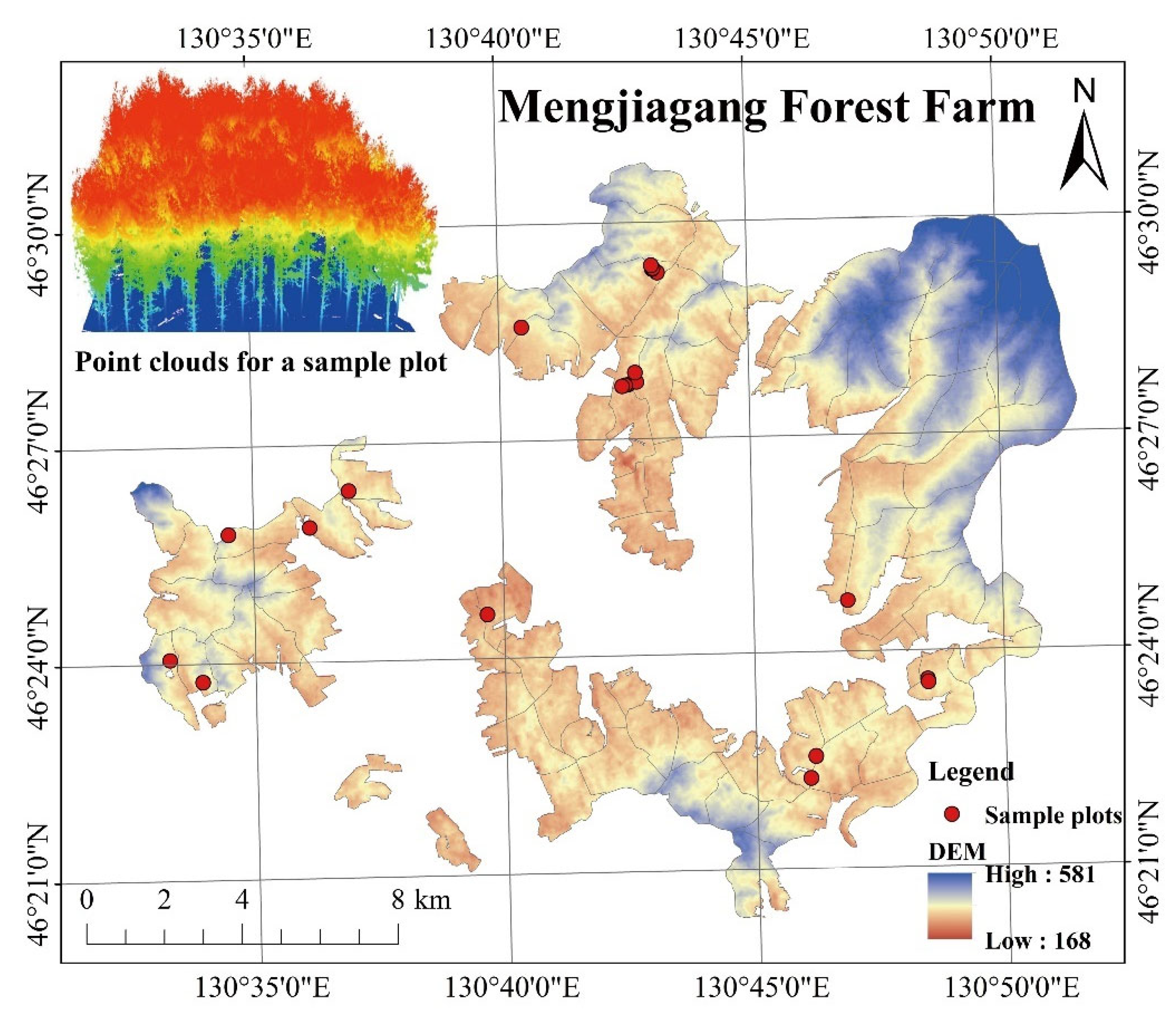
The study area is located in Mengjiagang Forest Farm, Jiamusi City, Heilongjiang Province, China (130°32′~130°52′ E, 46°20′~46°30′ N) (Figure 1), at the western foot of the Wanda Mountains. The landscape in this area is mainly low hills, and the slope is gradual, with an average elevation of 250 m. The area is characterized by an East Asian continental monsoon climate. The annual average temperature is 2.7 °C, and annual precipitation totals 550–670 mm. The soil type at this forest farm is primarily typical dark brown loam. Artificial forests cover 2/3 of the farm area, and the remaining 1/3 is covered with natural secondary forests. The study area has a forest coverage of 81.7%.
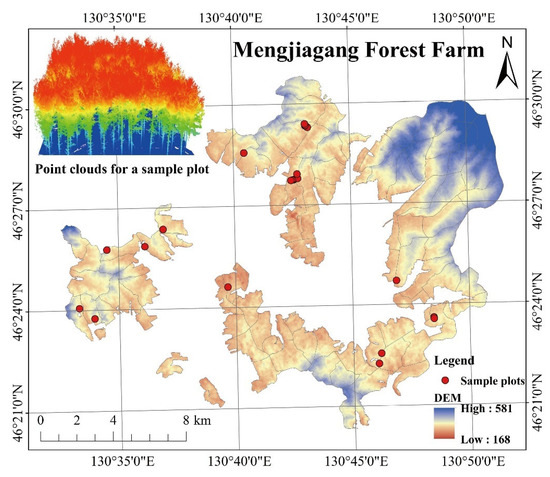
Figure 1.
Sample plots distribution map of Mengjiagang Forest Farm.
2.2. Field Measurements
In April 2020, we investigated 21 planted Korean pine plots (Table 1) at the Mengjiagang forest farm (Figure 1), each with different stand qualities, ages, and densities. All plots except plot 7 and 9 (0.09 ha) had an area of 0.06 ha. The center point coordinates of the plots were recorded using a GPS (GPSmap 621sc, GARMIN), and positioning accuracy was 3 m. Per-tree measurements were obtained for tree height, DBH, crown width, and first live branch height. An altimeter (Vertex IV, Haglöf Sweden, Sweden) was used to measure the trees’ height, a diameter tape was used to measure DBH, and a steel tape was used to measure crown width.

Table 1.
Sample plots information.
Jenkins et al. [57] noted that published biomass equations are available for the large-scale estimation of AGB. Therefore, our AGB reference values are calculated from Dong’s equation [58].
AGB = 0.2064 × DBH2.1169
2.3. Collecting TLS Data
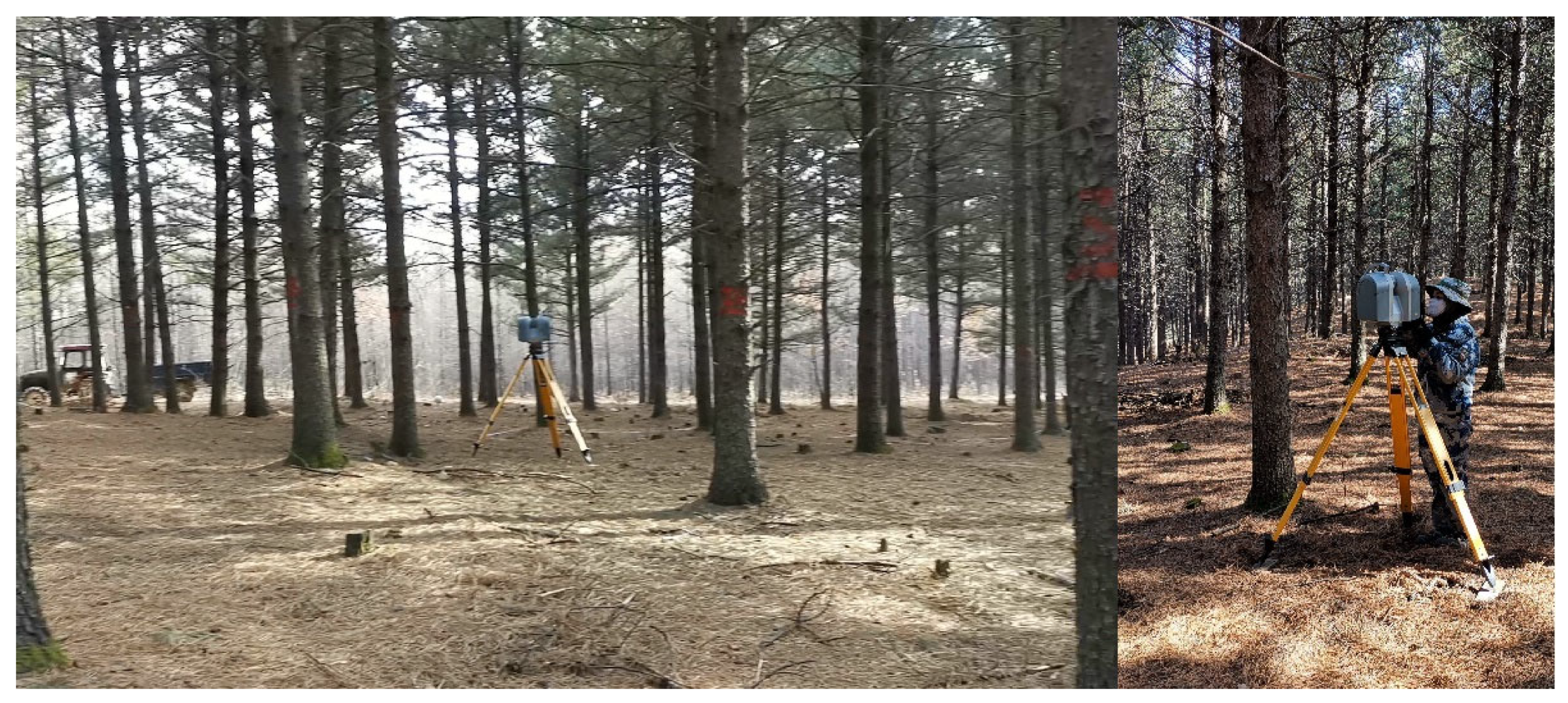
We obtained the point cloud data for 21 plots with a Trimble TX8 (Trimble, CA, USA). To ensure the comprehensiveness of the point cloud information for all trees in the plots, we performed scans with five stations in each plot. For more detail, one station was placed at the center of the plot and the scanning time set to 10 min. Four stations were placed at each of the four corners of the plot, and the scanning time was set to 3 min. Figure 2 depicts the details of the scanned plots.

Figure 2.
Picture of the TLS scan sample plots.
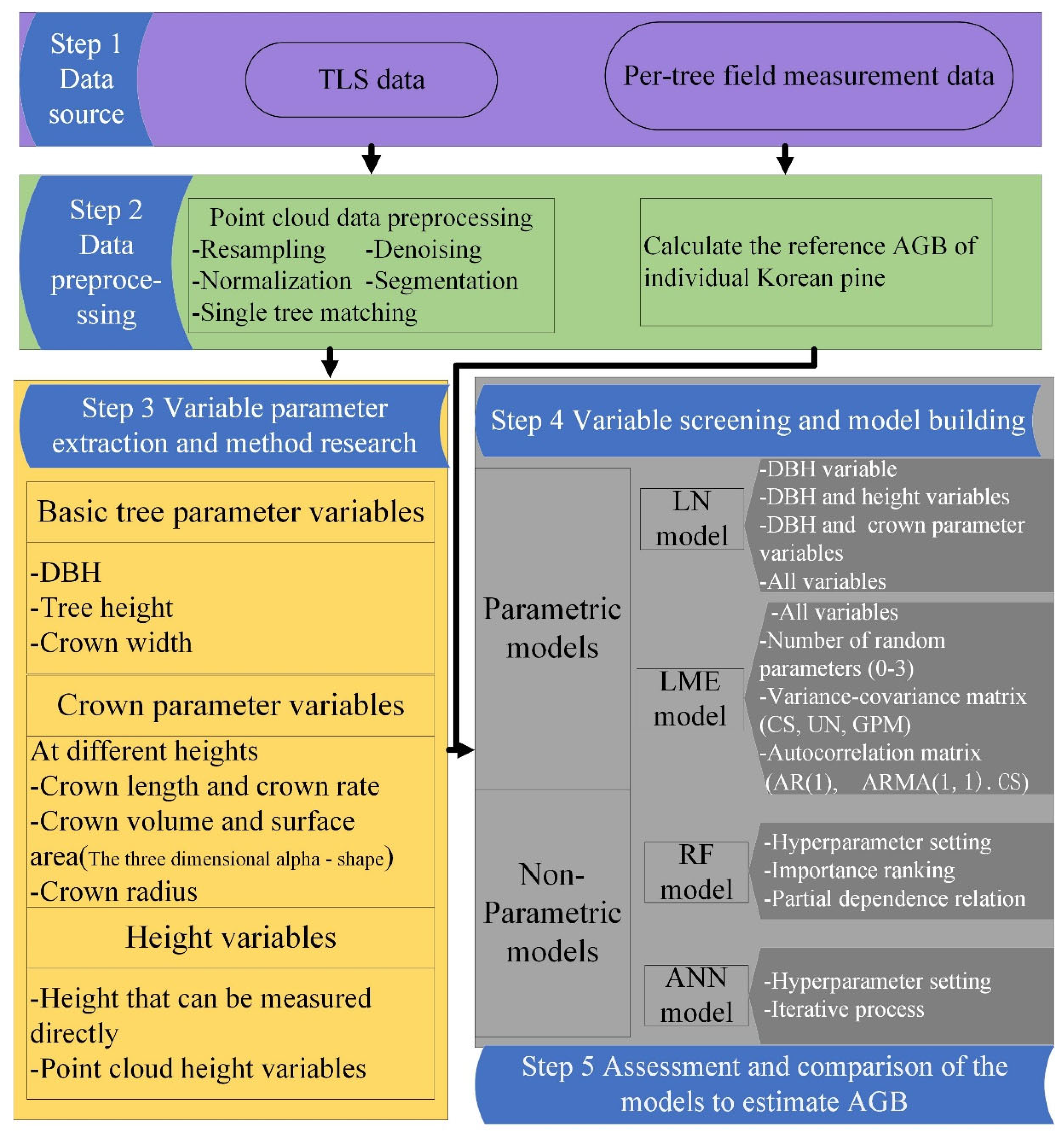
The point cloud data from multiple sites were input into Trimble RealWorks 11.2 (Trimble, CA, USA) software, and the target spheres were used as the marker for point cloud coregistration for each plot. Finally, the collocated point clouds were output in .las format. The point cloud density of each sample plot ranged from 20,000 points/m2 to 40,000 points/m2. More detailed processing was performed in LiDAR360 (Beijing Digital Green soil Technology Co., Ltd., Beijing, China) software. These processing tasks were as follows: point cloud cropping at the plot scale, point cloud resampling, denoising, point cloud data normalization, individual tree segmentation, and individual tree matching. Finally, we obtained the point cloud data of 1104 trees and divided them randomly into training and testing datasets in the ratio of 4:1. The specific process details of this study are shown in Figure 3.
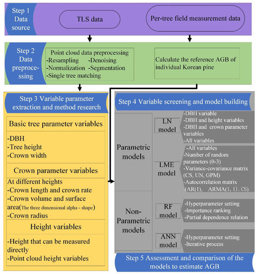
Figure 3.
Flow chart of this study.
2.4. Variable Extraction
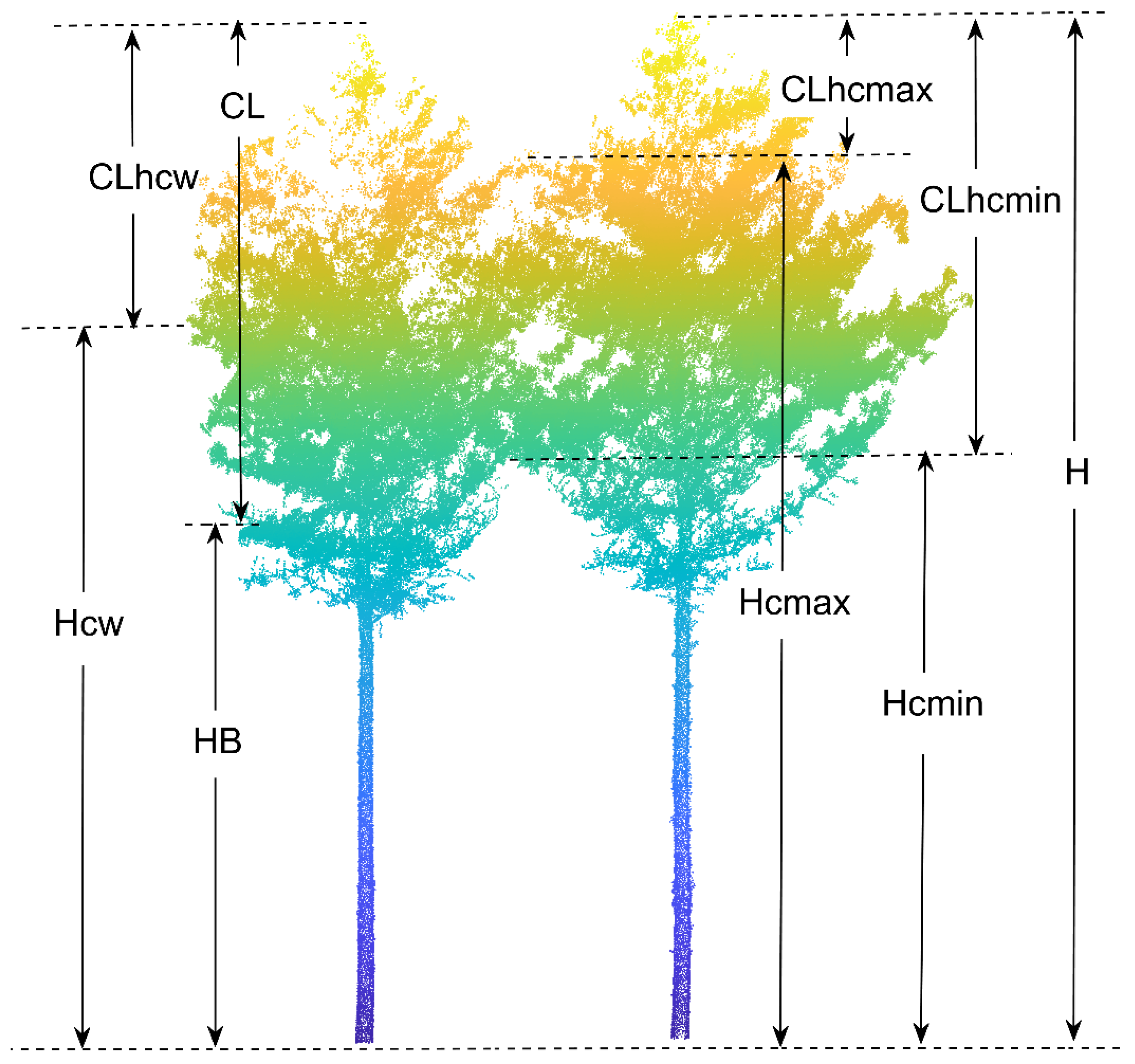
Both the waveform and point cloud data from TLS can visually and quantitatively reflect the vertical structure of forest stands. A more general approach toward estimating biomass is to develop regression relationships between variables such as point cloud height and field-measured stand height for large-scale extrapolation [59,60]. In this study, we extracted the height parameters from the normalized point cloud data for individual trees. Notably, data were obtained for parameters such as height percentile (Hp), mean height (Hmean), standard deviation of height (Hstd), variance of height (Hvar), median of height (Hmed), coefficient of variation of height (Hcv), interquartile spacing of height (Hiq), and skewness of height (Hskew). DBH, tree height, and crown width (CW) were also among the extracted variables. In addition, we extracted the first live branch height (HB), minimum contact height (Hcmin), maximum contact height (Hcmax), and height of crowns’ maximum width (Hcw) from the point clouds of individual trees based on a visual interpretation process (Figure 4). Moreover, the mean contact height (Hcmean), crown length (CL), crown length above the minimum contact height (CLhcmin), crown length above the maximum contact height (CLhcmax), crown length above the point of the maximum crown width (CLcw), and crown length ratio (CLr) were indirectly calculated with the above variables. A classification of the variables is given in Table 2, and a more detailed interpretation of the variables is provided in Table A1.
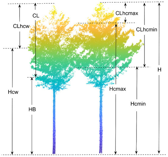
Figure 4.
Illustration of extracted variables. H is tree height, Hcmin is the minimum contact height, Hcmax is the maximum contact height, HB is the first living branch height, Hcw is the height of the maximum crown width, CLhcmin is the crown length above the minimum contact height, CLhcmax is the crown length above the maximum contact height, CL is crown length, and CLhcw is the crown length above the height of the maximum crown width.
Table 2.
List of variables extracted from TLS data.
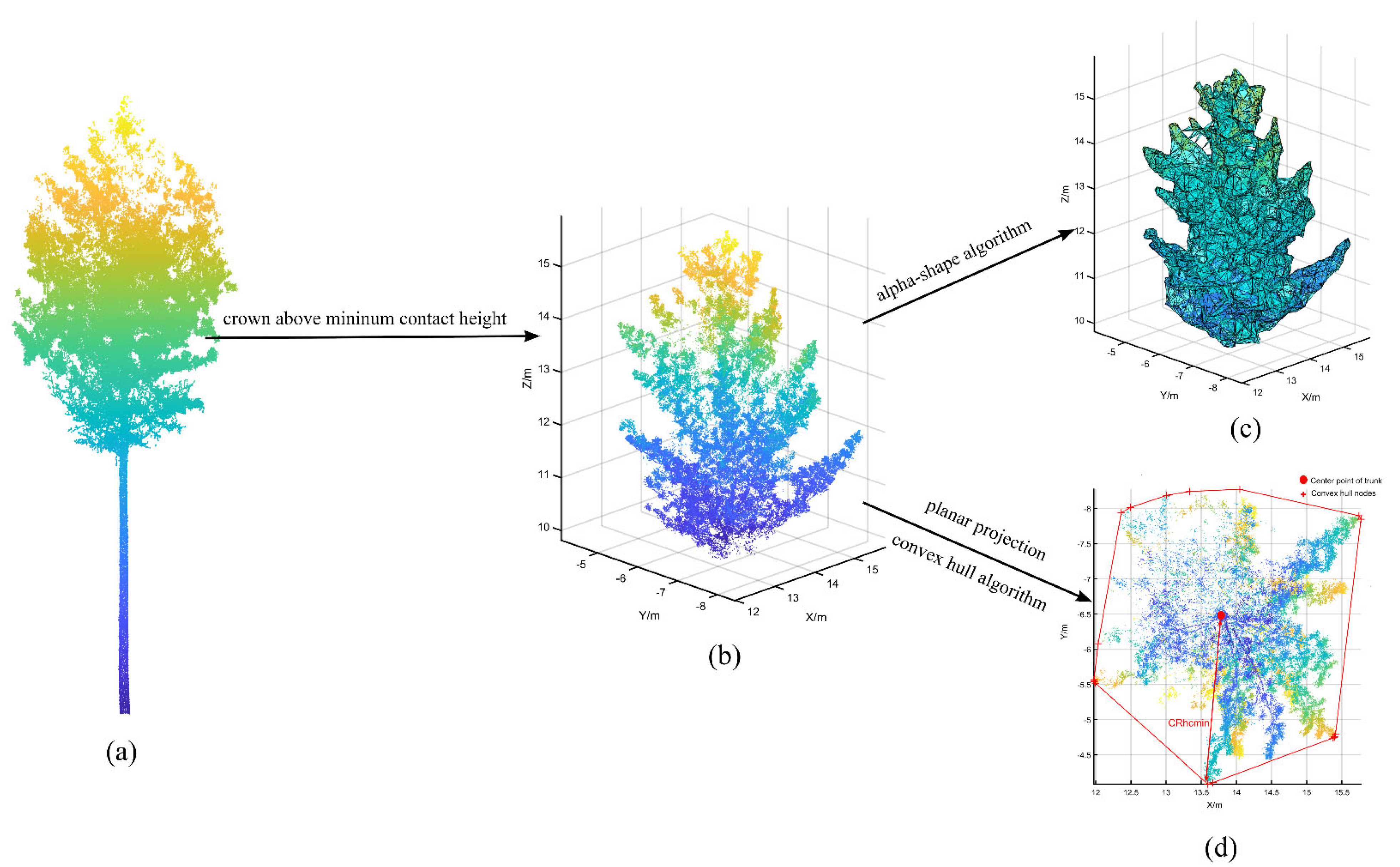
Crown structures above different contact heights can affect the AGB estimates for individual trees [23]. We extracted crown parameters for individual trees above different heights, such as the crown volume, crown surface area, and maximum crown radius above different contact heights. All crown parameters were extracted automatically in MATLAB R2020b (MathWorks, Natick, MA, USA) software. Notably, we automatically cropped the required crown point cloud (Figure 5b) according to the different height values and then applied the alpha-shape algorithm to reconstruct the crown surface (Figure 5c) and obtain the crown volume and surface area. The alpha-shape algorithm, first proposed by Edelsbrunner [61,62], is a classic edge detection algorithm that can be used to enhance or blur boundaries through parameter adjustments. Additionally, we performed a 2-D projection of the crown point cloud and applied the convex hull algorithm [63] to calculate the boundary points of the crown projection, which was useful for calculating the maximum crown radius at different heights (Figure 5d).
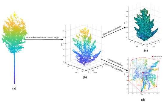
Figure 5.
Detailed process of crown parameter extraction above different heights; (a) is the complete point cloud for an individual Korean pine, (b) is the crown point cloud above the minimum contact height, (c) is the crown above the minimum contact height reconstructed with the alpha-shape algorithm, and (d) is the crown projection used to calculate the maximum crown radius.
2.5. Model Development
2.5.1. Linear Model
When establishing AGB equations based on the obtained TLS data, we used height parameters and crown parameters as independent variables and AGB calculated from field measurements as the dependent variable and selected the optimal explanatory variables in stepwise regression [64,65]. Four LN models were considered: one with DBH as the only independent variable (model 1); one with DBH and height parameters as independent variables (model 2); one with DBH and crown parameters as independent variables (model 3); and one in which all the extracted parameters were used as independent variables (model 4). SAS 9.4 (SAS Campus Drive, Cary, NC, USA.) software was used to run stepwise regressions. F tests were performed after each independent variable was introduced, and t tests were performed on each of the previously selected independent variables (t value was set to 0.05 in this study). Additionally, independent variables with variance inflation factors (VIF) greater than 10 were removed to limit the effect of independent variable collinearity on the modeling results.
2.5.2. Mixed-Effects Model
The mixed-effects model is suitable for studying the relationship between dependent and independent variables in grouped data, and its strong point is the flexibility in accounting for both the average trend in overall variations and the differences among individuals [66]. Our data were obtained from 1104 trees in 21 different plots and are very suitable for developing a mixed-effects model that can account for not only the average trends in individual-tree AGB across the study area but also the differences in individual-tree AGB among different plots with random effects. This approach can significantly enhance the accuracy of subsequent prediction models. An LME model of AGB at the plot level was developed based on the optimal LN model developed in Section 2.5.1. The LME model can be expressed as follows:
where is the observed AGB of the -th individual tree in the -th plot, is the model error term, is the number of plots, is the number of trees in each plot, and are known design matrices, is random-effects vector, and is fixed-effects vector. Model fitting was achieved with the ‘nlme’ package (https://cran.r-project.org/package=nlme, accessed on 10 January 2023) in R software.
2.5.3. Random Forest Model
A random forest (RF) is an integrated algorithm with a decision tree as the base learner [67]. In regression problems, RF models output a weighted average of the results obtained from all decision tree predictions as the final result [68]. In this study, an RF algorithm was applied to develop an individual-tree AGB estimation model with the selected optimal variables as inputs. We performed an automatic optimization search for the four hyperparameters considered most important in the RF algorithm: the number of decision trees (n_estimators), the minimum split sample size (min_samples_split), the minimum sample number of leaf nodes (min_samples_leaf), and the maximum number of separating features (max_features). Moreover, to avoid overfitting the trained model, the out-of-bag (OOB) error rate was used to verify the generalization ability of the model.
2.5.4. Artificial Neural Network Model
An artificial neural network (ANN) is a multilayered network consisting of several basic units connected by certain rules. In this study, an ANN model was developed with the Kears [69] deep learning framework to estimate the individual-tree AGB. We selected a 4-layer ANN with full connectivity between layers; the input layer included the filtered optimal variables, the middle two layers were hidden layers, and the output layer was the AGB of individual trees. The mean square error (MSE) was considered in the loss function. Rectified linear units (ReLUs) were applied in the activation function because the sigmoid function is influenced by extensive saturation, making gradient-based learning difficult; however, ReLUs display nearly linear behavior, leading to enhanced optimization and performance in most cases [70,71]. Moreover, to prevent overfitting, we applied an early termination strategy and set the maximum number of iterations in the model to 3000.
2.6. Model Evaluation
We evaluated the fitting and predictive abilities of the model based on independent test data with the coefficient of determination (R2), the absolute value of the mean relative error (RMAE), the root mean square error (RMSE), and the mean absolute error (MAE):
where is the observed value, is the predicted value, is the number of samples, and is the average of all the observed values.
3. Results
3.1. Linear Model of Individual-Tree AGB Based on TLS-Derived Parameters
The variables finally selected for each LN model and the coefficients of the variables are shown in Table 3. With DBH as the only independent variable in the model 1, it yields a lowest R2 for the test set. For the case with DBH and point cloud height parameters (model 2), DBH, Hp50, Hiq, and Hcmin were the final independent variables selected, and the R2 of model 2 is improved relative to model 1. For the case with DBH and crown structure parameters (model 3), DBH, CL, CLrhcmin, and Cscmin were selected as the independent variables, and model 3 produces the same results as model 2. In the fourth case, DBH, Hcmin, Cvcmin, Hstd, Crhcmin, and Hp1 were the selected variables (model 4), and model 4 performed best based on the test set. With detailed analysis, the independent variables of model 4 included not only crown structure parameters describing canopy information but also height parameters reflecting crown height information, which can better explain the changes in individual-tree AGB and be more accurately used to estimate individual-tree AGB than can other variables. Therefore, we finally chose model 4 as the optimal LN model for estimating individual-tree AGB.
Table 3.
Fitting results of linear models based on different variables.
3.2. Mixed-Effects Model for Individual-Tree AGB Based on TLS-Derived Parameters
Different combinations of random-effect parameter forms in model 4 were fitted using the ‘nlme’ package in R software. We selected the best random parameter combination form by comparing the fitness of each model considering the corresponding AIC, BIC, log likelihood, and R2 values. We also performed a likelihood ratio test (LRT) to avoid the problem of overparameterization. Significance tests were applied in this study and verified significant differences among the models when p < 0.05, as shown in Table 4 for the fitting results.
Table 4.
Fitting accuracy of the linear mixed-effects model based on different combinations of random-effect parameters.
Based on the results in Table 4, with the addition of random effects, the AIC and BIC of the model decreased compared to those of the LN model, and both the R2 and log likelihood values improved, which indicates that the LME model provides a better fit. The model 4–3 with random effects for a0, a1, and a3 yielded the minimum AIC and BIC, and both the log likelihood and R2 values of this model were maximums. The LRT results indicated significant differences among the models. Therefore, we finally selected model 4–3 as the optimal LME model for individual-tree AGB.
Table 5 shows the detailed results for each parameter in the optimal LN model and LME model for individual-tree AGB as well as the corresponding fitting statistics. AR (1) is the optimal matrix for describing the autocorrelation structure in the LME model.
Table 5.
Fitting results for the optimal linear model and linear mixed-effects models.
3.3. Random Forest Model for Individual-Tree AGB Based on TLS-Derived Parameters
3.3.1. Optimal Hyperparameters
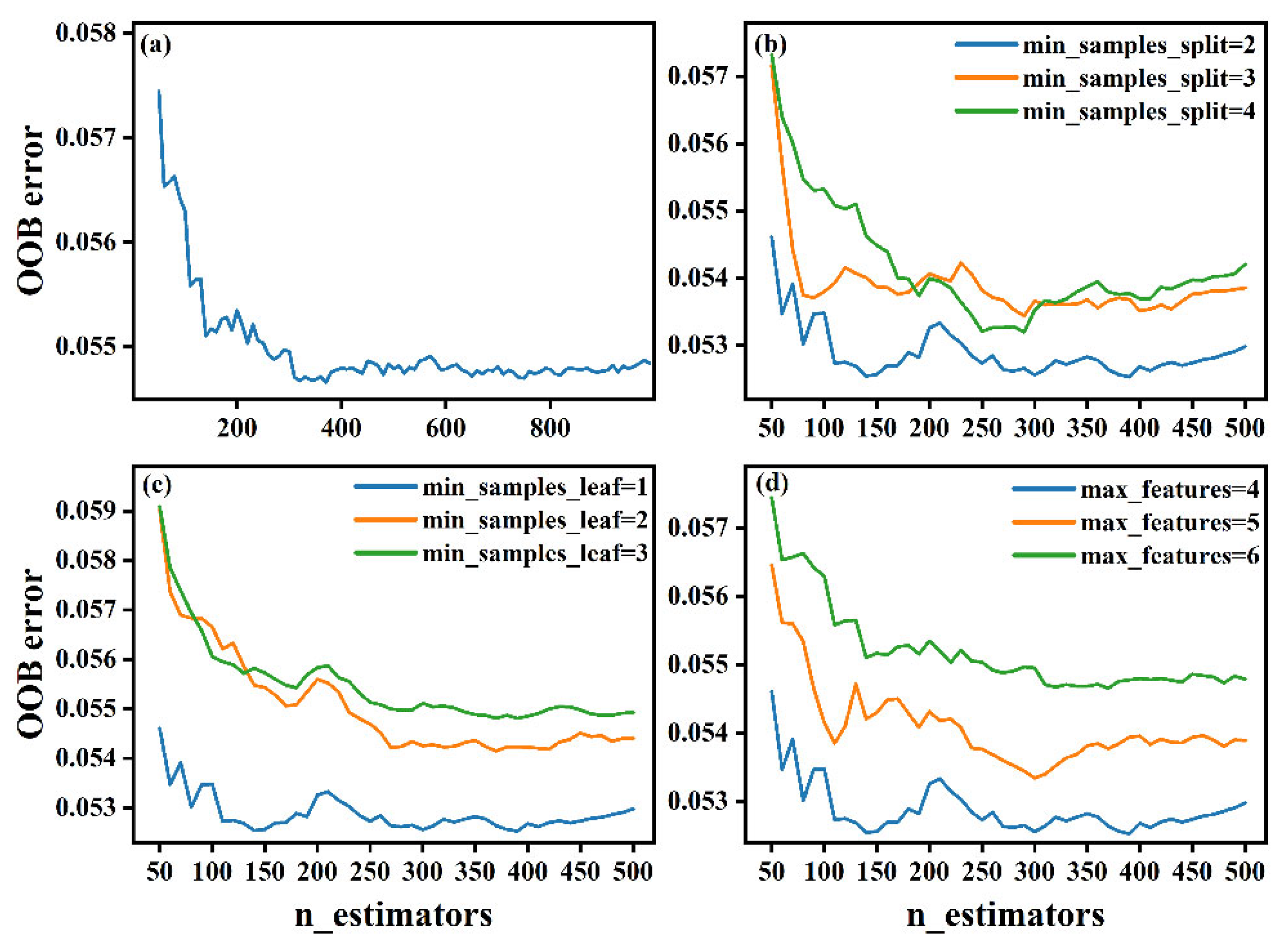
Figure 6a shows the effect of n_estimators on the OOB error; notably, the model yields the minimum OOB error when n_estimators is equal to 390. The effects of min_samples_split, min_samples_leaf, and max_features on the OOB error are shown in Figure 6b–d, respectively. Finally, the optimal hyperparameters of the RF model are chosen as n_estimators = 390, min_samples_split = 2, min_samples_leaf = 1, and max_features = 4.
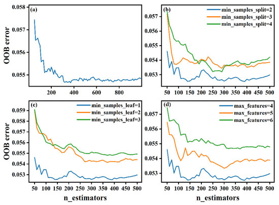
Figure 6.
Graph of the OOB error for the RF model with different hyperparameter combinations. (a) none, (b) min_samples_split, (c) min_samples_leaf, (d) max_features.
3.3.2. Relative Importance and Partial Dependence
The RF model can be used to determine the relative importance of the independent variables and to produce a partial dependence plot for the dependent variable [67] driven by the independent variables, which are crucial elements in enhancing the interpretability of RF results. Partial dependence plots aid in visualizing the dependence of the outcome on the independent variables. One point worth emphasizing is that we cannot ignore the effects of other variables on the dependent variable when calculating dependence and instead should consider the average effect of all variables on the dependent variable.
Figure 7 illustrates the relative importance of the effects of each independent variable on the individual-tree AGB. It is obvious that DBH is the primary factor influencing AGB, with a relative importance of 66.47%. Height parameters and crown structure parameters also have some effect on individual-tree AGB, with a total relative importance of 33.53%. The relative importance of each variable in relation to individual-tree AGB is ranked as follows: DBH > Hcmin > Hstd > Cvcmin > Crhcmin > Hp1.
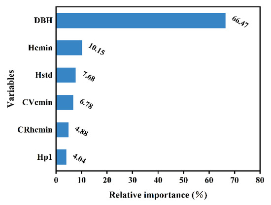
Figure 7.
Relative importance of each independent variable in the RF model.
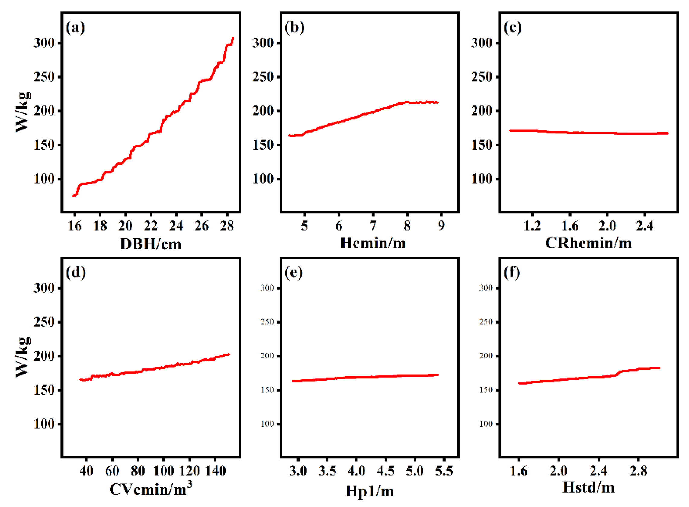
The partial dependence of individual-tree AGB on each independent variable is plotted in Figure 8. There was a strong dependence between individual-tree AGB and DBH, as also observed for the relative importance of variables in Figure 7. Hcmin, Hstd, and Cvcmin also display dependence relations with individual-tree AGB. Additionally, for Crhcmin and Hp1, only very weak dependence relations with AGB are observed, as shown in Figure 8.
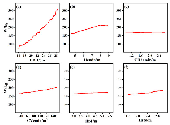
Figure 8.
Partial dependence plots of each independent variable affecting individual-tree AGB change. (a) DBH, (b) Hcmin, (c) CRhcmin, (d) CVcmin, (e) Hp1, (f) Hstd.
3.4. Artificial Neural Network Model for Individual-Tree AGB Based on TLS-Derived Parameters
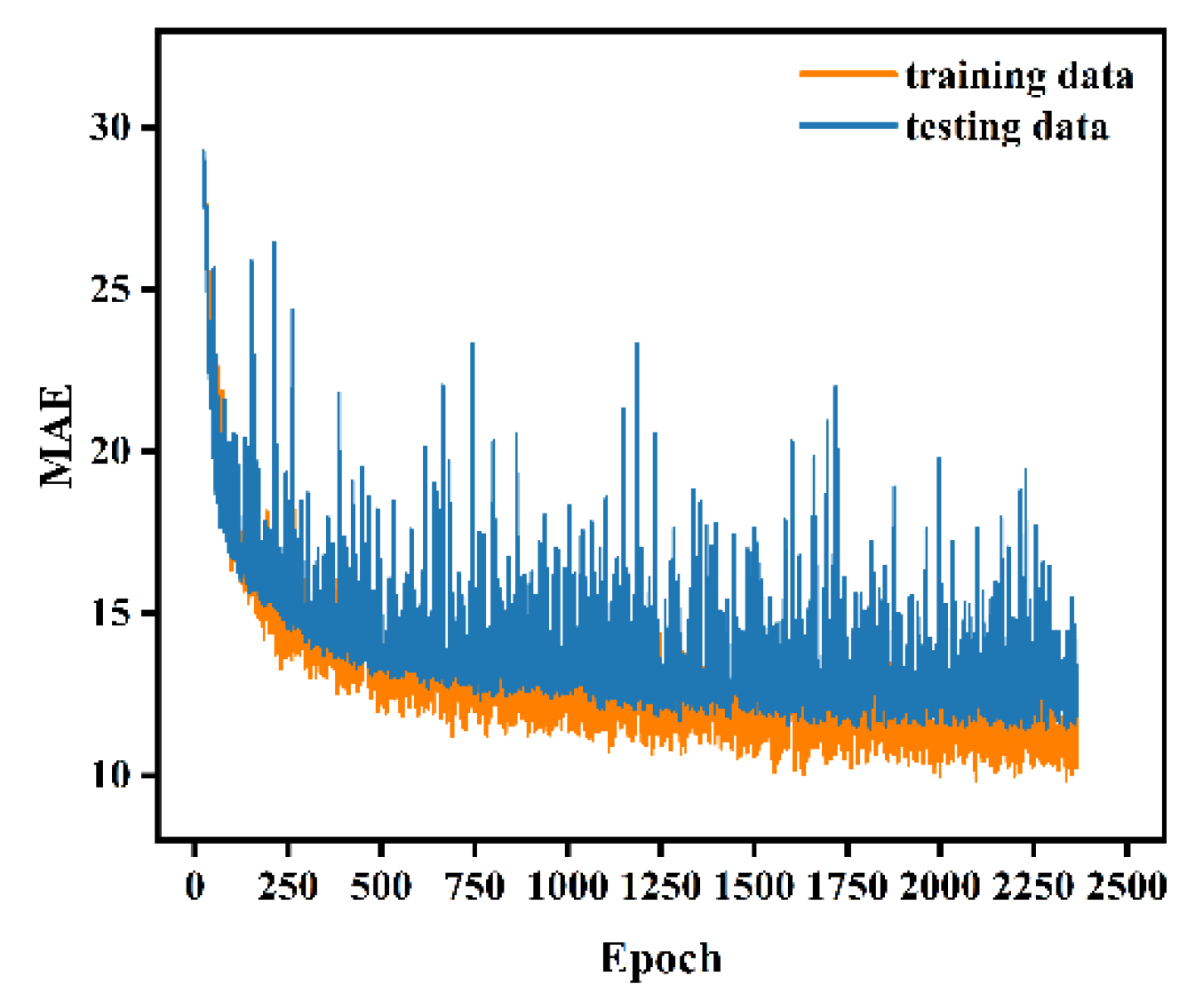
The ANN model was built with the variables DBH, Hcmin, Cvcmin, Hstd, Crhcmin, and Hp1 in the input layer. The variable in the output layer was the individual-tree AGB, the number of neurons in each hidden layer was set to 64, and the layers were fully connected to each other. Other parameters of the model were set as follows: initial learning rate was 0.001, dropout was 0.02, batch size was 32, and maximum number of iterations was 3000. The iterative process of fitting the ANN model is illustrated in Figure 9. Notably, the fitting effect of the model for the training set is not much different than that for the test set, which suggests that no overfitting occurs. Additionally, the model achieves the optimal fitting effect at epoch 2369. The ANN model yields an R2 of 0.969 and an RMSE of 16.161 kg for the training set and an R2 of 0.952 and an RMSE of 15.897 kg for the test set.
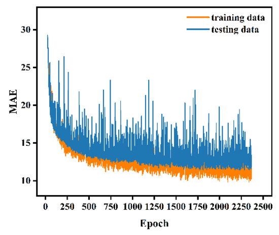
Figure 9.
Iterative process of the ANN model.
3.5. Model Comparison
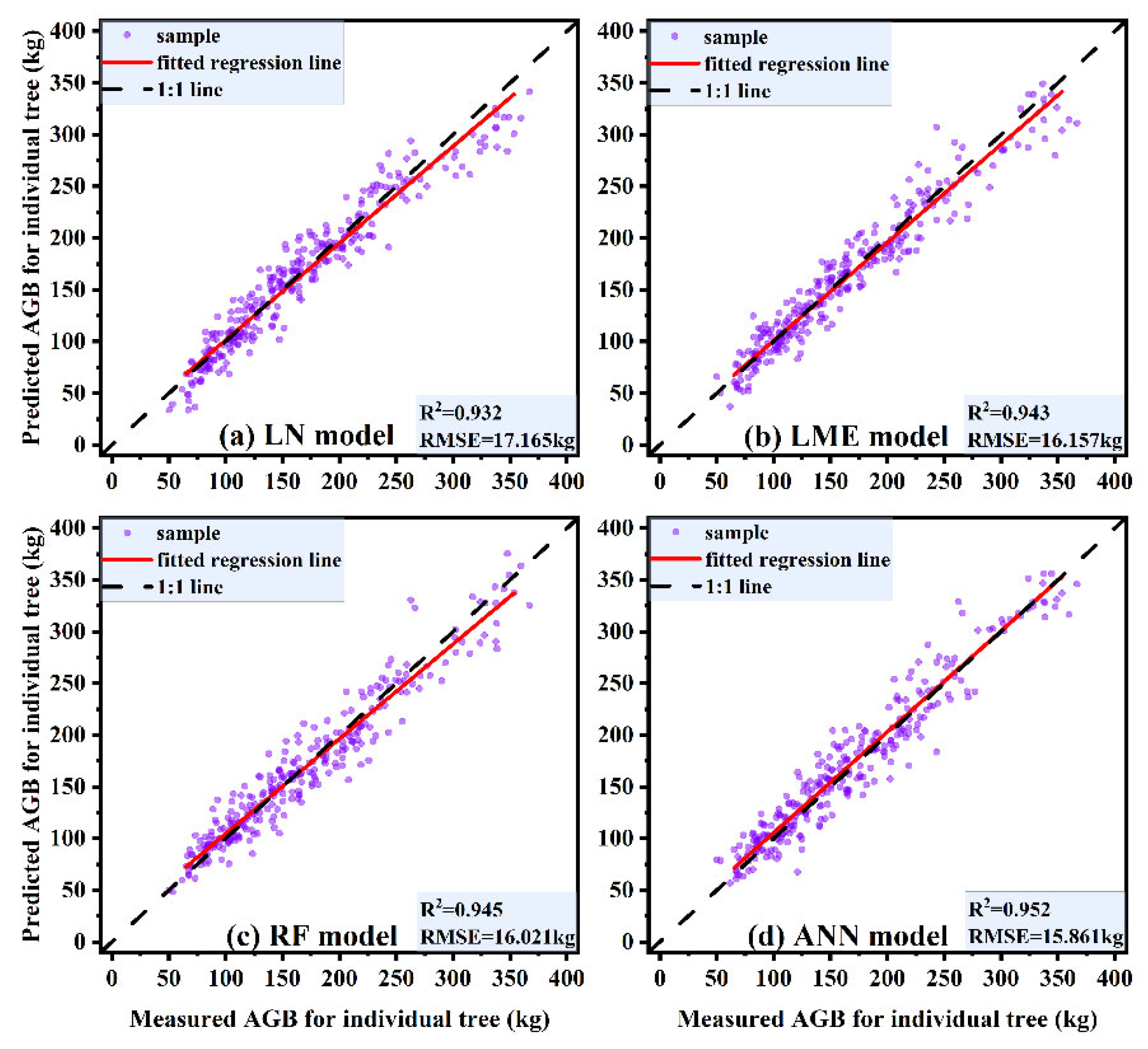
Table 6 shows the fitting results of each model for the training set and the prediction results for the independent test set. It is obvious that the evaluation indexes of the models do not differ significantly for different data sets, which suggests that none of the models are influenced by overfitting. All models provide acceptable prediction ability, with R2 values above 0.932 and RMSEs below 17.165 kg. The ANN model provides the best prediction ability. Compared with the other three models, the ANN model yields R2 improvements of 2.15%, 0.95%, and 0.74%, the RMSE is reduced by 5.06%, 3.55%, and 2.77%, and the MAE is reduced by 6.58%, 4.31%, and 0.45%, respectively. The predictive accuracy of each model can be ranked as follows: ANN model > RF model > LME model > LN model.
Table 6.
Fitting and prediction abilities of the optimal models.
4. Discussion
Information about tree crowns above different contact heights was extracted in this study from TLS, and such information is generally not provided by traditional methods. After analysis, we concluded that adding crown information above different contact heights to an individual-tree AGB model can improve the estimation accuracy of the model, which is consistent with the results of Zheng et al. [23]. One limitation is that in this paper, a visual interpretation method was applied to extract the crown contact height; therefore, determining how to automatically extract the contact heights of different individual trees is an urgent problem that must be addressed in future research. We applied the 3D alpha-shape algorithm to reconstruct the crown above different contact heights, and the parameters were adjusted to make the crown boundary more detailed and unaffected by the point cloud density inside the crown. Therefore, the crown volume extracted using the 3D alpha-shape algorithm was closer to the true value [72] than the extraction results obtained would be with the convex-hull algorithm [73,74] or fixed-size voxel method [75,76].
The waveform or point cloud data from TLS can visually and quantitatively reflect the vertical structure of the forest community. A more general approach to estimating AGB is to establish regression relationships between variables such as the height of point clouds and the field-measured forest community height for large-scale extrapolation [68,77], and few studies have reported AGB estimates at the individual-tree scale based on the height parameters from point clouds. We extracted the height parameters from the normalized point cloud data for individual trees and revealed that they can be considered independent variables in individual-tree AGB prediction models after a stepwise regression method is applied to select variables. Our results show that TLS can provide valuable variable information for developing individual-tree AGB models without destroying trees as a way to improve the accuracy of individual-tree AGB estimates. Consequently, a valid proposal is that in future research, we should fully utilize the nondestructive data acquisition capability of TLS to provide additional valuable information for the development of forest biomass and carbon stock prediction models as a way to strengthen the predictions of forest biomass and carbon stock models.
In some recent studies, individual-tree AGB models have been developed with TLS-derived parameters [46,78,79,80], and these authors concluded that considering crown parameters and height parameters can improve the accuracy of individual-tree AGB estimation. In this paper, we developed four individual-tree AGB LN models using the parameters derived from TLS (Table 3). The results showed that: the models incorporating height parameters (model 2) or crown parameters (model 3) performed better than those with only DBH as the independent variable (model 1); the models incorporating height parameters (model 2) offered better predictions than those incorporating crown parameters (model 3); and the highest prediction accuracy was achieved when both height parameters and crown parameters were included in the model (model 4), in accordance with the results of previous research. However, the crown parameters included in the individual-tree AGB models of other researchers were typically crown volume [78], crown surface area [46], and crown diameter, which are all from the whole crown [79,80]. In contrast, the crown parameters included in the optimal individual-tree AGB LN model (model 4) developed in our study are Cvcmin and Crhcmin, representing the crown information above the minimum contact height. Zheng et al. [23] reported a strong correlation between larch crown parameters above the minimum contact height and individual-tree AGB. Wang et al. [24] proposed a new physical parameter, the LBI, and obtained robust individual-tree AGB estimates by combining the LBI with the traditional allometric growth equation. It is worth emphasizing that the LBI includes crown information above different contact heights. The results of all of these works suggest that considering crown information above different contact heights contributes to improving estimates of individual-tree AGB, and therefore, developing AGB models based on crown information above the contact height of individual trees is certainly scientifically reasonable. In addition, ALS takes a top-down approach, which is less capable of acquiring information from the lower part of the canopy, while it can accurately acquire information from the upper part of the canopy [81]. Thus, the individual-tree AGB prediction model we developed that includes crown information above the minimum contact height is also applicable to ALS data, and our model provides a novel approach to estimating individual-tree AGB at large scales using ALS.
Different models could have a certain impact on the prediction accuracy of individual-tree AGB. Parametric models are commonly used in traditional approaches for individual-tree AGB prediction [11,48,50], and they can clearly and intuitively reflect the relationship between AGB and each independent variable; however, parametric models are usually not highly accurate. Scholars have applied machine learning methods in conjunction with individual-tree AGB models [52,53] and developed nonparametric models for estimating individual-tree AGB, such models include RF and ANN models, among others. The use of nonparametric models can improve the accuracy of AGB prediction to some extent; nevertheless, it is difficult to explain the relationship between independent variables and AGB. In this paper, we compared the estimation of individual-tree AGB based on parametric models (LN and LME models) and nonparametric models (RF and ANN models). The 1:1 scatter plot of the predicted and measured values of individual-tree AGB (Figure 10) clearly displays the results, with the predictive ability of each model ranked as follows: ANN model > RF model > LME model > LN model. The LN model, as the most commonly applied biomass prediction model, is simple and can be used to efficiently determine the extent to which AGB is influenced by the relevant independent variables. The average trend of the overall individual-tree AGB within a region can be inferred using an LN model, but the differences among separate small areas within a region are ignored, and the prediction accuracy is often limited. The LME model is divided into two parts: fixed effects and random effects [66]. Fixed effects can describe the average trend of overall individual-tree AGB in the region, while random effects can complement the description of the differences in individual-tree AGB among various small areas in the region, making the LME model very flexible and providing comparatively accurate predictions of individual-tree AGB. There are also drawbacks to the LME model; notably, the random-effects parameters and variance structure must be properly set. Consequently, the model is computationally complex and not easy to apply in practical cases. RF and ANN models, as two of the currently popular nonparametric models available, have been relatively well established for forestry applications [52,53,55,56]. Based on the comparison, we can conclude that these two nonparametric models have improved the accuracy of individual-tree AGB prediction more than have traditional parametric models. Moreover, nonparametric models have simple data structure requirements, and the algorithms are flexible and efficient, making them ideal for practical applications. The ANN model yielded the highest accuracy in individual-tree AGB prediction in this study, followed by the RF model. However, the ANN model is based on a ‘black box’ operation when making individual-tree AGB predictions, and the prediction process cannot be clearly visualized; therefore, we cannot fully assess the accuracy of the prediction results. Although the RF model produces lower prediction accuracy than the ANN model, the RF results are much more interpretable. Specifically, relative importance plots and partial dependence plots of the independent variables can be easily produced. Therefore, overall, we recommend the RF model as the optimal individual-tree AGB prediction model for practical applications.
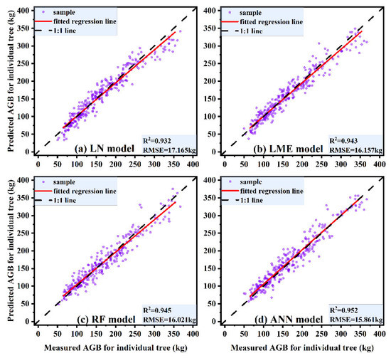
Figure 10.
1:1 scatter plots of estimated and measured values of individual-tree AGB for different models. (a) LN model, (b) LME model, (c) RF model, (d) ANN model.
5. Conclusions
TLS is playing an ever more critical role in forestry applications as an active remote sensing technology. In this paper, we show that TLS can be used to accurately estimate individual-tree AGB. We extracted height parameters and crown structure parameters at different heights from the point clouds of 1104 planted Korean pine and introduced these variables into an individual-tree AGB estimation model. The results showed that the predictive ability of the model was improved with this approach, especially by adding the crown structure parameters above the minimum contact height. This finding verifies that the crown above the minimum contact height is an important factor in individual-tree AGB estimation, and it may be related to the effective crown. In addition, TLS is used to obtain crown structure parameters and is nondestructive, precise, and repeatable; therefore, it can be considered in future research to monitor plots over multiple periods and achieve the dynamic monitoring of forest biomass and carbon stock changes.
Finally, we compared the ability of the LN, LME, RF, and ANN models to estimate individual-tree AGB. Overall, the predictive ability of the models was ranked as follows: ANN model > RF model > mixed-effects model > linear model. This result demonstrated that the nonparametric models performed better than the other models in individual-tree AGB prediction. Nonparametric models are based on flexible algorithms and have no data structure requirements; thus, they are widely used in forestry. In this paper, both ANN and RF models yielded accurate estimates of individual-tree AGB. The ANN model uses a ‘black box’ operation in the prediction process, but the RF model provides more interpretable results; therefore, we recommend the RF model as the optimal model for estimating individual-tree AGB.
Author Contributions
Conceptualization, F.W., Y.S. and W.J.; methodology, F.W.; software, F.W.; validation, F.W., Y.S. and D.L.; formal analysis, F.W.; investigation, W.Z., H.G., Y.T. and X.Z.; data curation, F.W. and Y.T.; writing—original draft preparation, F.W.; writing—review and editing, F.W. and W.J.; supervision, W.J.; project administration, W.J.; funding acquisition, W.J. All authors have read and agreed to the published version of the manuscript.
Funding
This research was funded by the Regional Innovation and Development of the National Natural Science Foundation of China (Grant No. U21A20244), Special Fund Project for Basic Research in Central Universities (Grant No. 2572019CP08) and the Natural Science Foundation of China (Grant No. 31870622).
Data Availability Statement
Not applicable.
Conflicts of Interest
The authors declare no conflict of interest.
Appendix A
Table A1.
Detailed interpretation of the crown parameters.
Table A1.
Detailed interpretation of the crown parameters.
| Variables | Interpretation |
|---|---|
| CL | Crown length |
| CLr | Crown ratio (CL/H) |
| CLcw | The length of crown above the height where maximum crown width is measured |
| CLrcw | The ratio of crown above the height where maximum crown width is measured (CLcw/H) |
| CLhcmin | The length of crown above the minimum height of the target crown contact with the adjacent crown |
| CLrhcmin | The ratio of crown above the minimum height of the target crown contact with the adjacent crown (CLhcmin/H) |
| CLhcmean | The length of crown above the mean height of the target crown contact with the adjacent crown |
| CLrhcmean | The ratio of crown above the mean height of the target crown contact with the adjacent crown (CLhcmean/H) |
| CLhcmax | The length of crown above the maximum height of the target crown contact with the adjacent crown |
| CLrhcmax | The ratio of crown above the maximum height of the target crown contact with the adjacent crown (CLhcmax/H) |
| CVcw | The volume of crown above the height where maximum crown width is measured |
| CScw | The surface area of crown above the height where maximum crown width is measured |
| CVhcmin | The volume of crown above the minimum height of the target crown contact with the adjacent crown |
| CShcmin | The surface area of crown above the minimum height of the target crown contact with the adjacent crown |
| CVhcmean | The volume of crown above the mean height of the target crown contact with the adjacent crown |
| CShcmean | The surface area of crown above the mean height of the target crown contact with the adjacent crown |
| CVhcmax | The volume of crown above the maximum height of the target crown contact with the adjacent crown |
| CShcmax | The surface area of crown above the maximum height of the target crown contact with the adjacent crown |
| CW | Maximum crown width |
| CRhcmin | Crown radius at minimum height of the target crown contact with the adjacent crown |
| CRhcmean | Crown radius at mean height of the target crown contact with the adjacent crown |
| CRhcmax | Crown radius at maximum height of the target crown contact with the adjacent crown |
| HB | Height of first live branch |
| Hcw | Height where the maximum crown width is measured |
| Hcmin | Minimum height of the target crown contact with the adjacent crown |
| Hcmean | Mean height of the target crown contact with the adjacent crown |
| Hcmax | maximum height of the target crown contact with the adjacent crown |
| Hp1~Hp99 | Percentile of height in normalized point cloud (1%, 5%, 10%, 20%, 25%, 30%, 40%, 50%, 60%, 70%, 75%, 80%, 90%, 95%, 99%) |
| Hmax | Maximum value of height in the normalized point cloud |
| Hmean | Mean value of height in the normalized point cloud |
| Hmin | Maximum value of height in the normalized point cloud |
| Hmed | Median of height in the normalized point cloud |
| Hstd | Standard deviation of height in the normalized point cloud |
| Hvar | Variance of height in the normalized point cloud |
| Hcv | Coefficients of variation of height in the normalized point cloud |
| Hskew | Skewness of height in the normalized point cloud |
| Hiq | Interquartile spacing of height percentile in the normalized point cloud |
References
- Dong, L.H.; Li, F.R. Stand-level biomass estimation models for the tree layer of main forest types in East Daxing’an Mountains, China. Chin. J. Appl. Ecol. 2018, 29, 2825–2834. [Google Scholar]
- Asrat, Z.; Eid, T.; Gobakken, T.; Negash, M. Aboveground tree biomass prediction options for the Dry Afromontane forests in south-central Ethiopia. For. Ecol. Manag. 2020, 473, 118335. [Google Scholar] [CrossRef]
- Ter-Mikaelian, M.T.; Korzukhin, M.D. Biomass equations for sixty-five North American tree species. For. Ecol. Manag. 1997, 97, 1–24. [Google Scholar] [CrossRef]
- Wang, J.; Zhang, L.; Feng, Z. Allometric Equations for the Aboveground Biomass of Five Tree Species in China Using the Generalized Method of Moments. For. Chron. 2018, 94, 7. [Google Scholar]
- Roxburgh, S.H.; Paul, K.I.; Clifford, D.; England, J.R.; Raison, R.J. Guidelines for constructing allometric models for the prediction of woody biomass: How many individuals to harvest? Ecosphere 2015, 6, 1–27. [Google Scholar] [CrossRef]
- Repola, J. Biomass equations for Scots pine and Norway spruce in Finland. Silva Fenn. 2009, 43, 184. [Google Scholar] [CrossRef]
- Lefsky, M.A. Application of Lidar Remote Sensing to the Estimation of Forest Canopy and Stand Structure; UMI: Ann Arbor, MI, USA, 1997. [Google Scholar]
- Musthafa, M.; Singh, G. Forest above-ground woody biomass estimation using multi-temporal space-borne LiDAR data in a managed forest at Haldwani, India. Adv. Space Res. 2022, 69, 3245–3257. [Google Scholar] [CrossRef]
- Pastor, J.; Aber, J.D.; Melillo, J.M. Biomass prediction using generalized allometric regressions for some northeast tree species. For. Ecol. Manag. 1984, 7, 265–274. [Google Scholar] [CrossRef]
- Kuyah, S.; Dietz, J.; Muthuri, C.; van Noordwijk, M.; Neufeldt, H. Allometry and partitioning of above- and below-ground biomass in farmed eucalyptus species dominant in Western Kenyan agricultural landscapes. Biomass-Bioenergy 2013, 55, 276–284. [Google Scholar] [CrossRef]
- Huy, B.; Kralicek, K.; Poudel, K.P.; Phuong, V.T.; Van Khoa, P.; Hung, N.D.; Temesgen, H. Allometric equations for estimating tree aboveground biomass in evergreen broadleaf forests of Viet Nam. For. Ecol. Manag. 2016, 382, 193–205. [Google Scholar] [CrossRef]
- Täll, K. Accuracy of Mobile Forest Inventory Application KatamTM Forest. Second Cycle, A2E; Southern Swedish Forest Research Centre, SLU: Alnarp, Sweden, 2020. [Google Scholar]
- Mankou, G.S.; Ligot, G.; Panzou, G.J.L.; Boyemba, F.; Loumeto, J.J.; Ngomanda, A.; Obiang, D.; Rossi, V.; Sonke, B.; Yongo, O.D.; et al. Tropical tree allometry and crown allocation, and their relationship with species traits in central Africa. For. Ecol. Manag. 2021, 493, 119262. [Google Scholar] [CrossRef]
- Kükenbrink, D.; Gardi, O.; Morsdorf, F.; Thürig, E.; Schellenberger, A.; Mathys, L. Above-ground biomass references for urban trees from terrestrial laser scanning data. Ann. Bot. 2021, 128, 709–724. [Google Scholar] [CrossRef]
- Feng, Z.; Luo, X.; Ma, Q.Y.; Hao, X.Y.; Chen, X.X.; Zhao, L.G. An estimation of tree canopy biomass based on 3D laser scanning imaging system. J. Beijing For. Univ. 2007, 29, 52–56. [Google Scholar]
- Evangelista, P.; Kumar, S.; Stohlgren, T.J.; Crall, A.W.; Newman, G.J. Modeling Aboveground Biomass of Tamarix Ramosissima in the Arkansas River Basin of Southeastern Colorado, USA. West. N. Am. Nat. 2007, 67, 503–509. [Google Scholar] [CrossRef]
- Zhang, H.R.; Tang, S.Z.; Wang, F.Y. Study on Estabilish and Estimate Method of Biomass Model Compatible with Volume. For. Res. 1999, 12, 56–62. [Google Scholar]
- Huang, X.Z.; Sun, X.M.; Zhang, S.G.; Chen, D. Compatible Biomass Models for Larix kaempferi in Mountainous Area of Eastern Liaoning. For. Res. 2014, 27, 142–148. [Google Scholar] [CrossRef]
- Goodman, R.C.; Phillips, O.L.; Baker, T.R. The importance of crown dimensions to improve tropical tree biomass estimates. Ecol. Appl. 2014, 24, 680–698. [Google Scholar] [CrossRef]
- Wang, M.; Im, J.; Zhao, Y.; Zhen, Z. Multi-Platform LiDAR for Non-Destructive Individual Aboveground Biomass Estimation for Changbai Larch (Larix olgensis Henry) Using a Hierarchical Bayesian Approach. Remote Sens. 2022, 14, 4361. [Google Scholar] [CrossRef]
- Wang, M.; Liu, Q.; Fu, L.; Wang, G.; Zhang, X. Airborne LIDAR-Derived Aboveground Biomass Estimates Using a Hierarchical Bayesian Approach. Remote Sens. 2019, 11, 1050. [Google Scholar] [CrossRef]
- Li, F.R.; Wang, Z.F.; Wang, B.S. Studies on the effective crown development of larix olgensis (I)-determination of the effective crown. J. Northeast For. Univ. 1996, 24, 1–8. [Google Scholar]
- Zheng, Y.; Jia, W.; Wang, Q.; Huang, X. Deriving Individual-Tree Biomass from Effective Crown Data Generated by Terrestrial Laser Scanning. Remote Sens. 2019, 11, 2793. [Google Scholar] [CrossRef]
- Wang, Q.; Pang, Y.; Chen, D.; Liang, X.; Lu, J. Lidar biomass index: A novel solution for tree-level biomass estimation using 3D crown information. For. Ecol. Manag. 2021, 499, 119542. [Google Scholar] [CrossRef]
- Disney, M.I.; Vicari, M.B.; Burt, A.; Calders, K.; Lewis, S.L.; Raumonen, P.; Wilkes, P. Weighing trees with lasers: Advances, challenges and opportunities. Interface Focus 2018, 8, 20170048. [Google Scholar] [CrossRef]
- Hudak, A.T.; Strand, E.K.; Vierling, L.A.; Byrne, J.C.; Eitel, J.U.; Martinuzzi, S.; Falkowski, M.J. Quantifying aboveground forest carbon pools and fluxes from repeat LiDAR surveys. Remote Sens. Environ. 2012, 123, 25–40. [Google Scholar] [CrossRef]
- Ahmed, R.; Siqueira, P.; Hensley, S. A study of forest biomass estimates from lidar in the northern temperate forests of New England. Remote Sens. Environ. 2013, 130, 121–135. [Google Scholar] [CrossRef]
- Lim, K.; Treitz, P.; Wulder, M.; St-Onge, B.; Flood, M. LiDAR remote sensing of forest structure. Prog. Phys. Geogr. Earth Environ. 2003, 27, 88–106. [Google Scholar] [CrossRef]
- Dassot, M.; Constant, T.; Fournier, M. The use of terrestrial LiDAR technology in forest science: Application fields, benefits and challenges. Ann. For. Sci. 2011, 68, 959–974. [Google Scholar] [CrossRef]
- Fernández-Sarría, A.; Martínez, L.; Velázquez-Martí, B.; Sajdak, M.; Estornell, J.; Recio, J. Different methodologies for calculating crown volumes of Platanus hispanica trees using terrestrial laser scanner and a comparison with classical dendrometric measurements. Comput. Electron. Agric. 2012, 90, 176–185. [Google Scholar] [CrossRef]
- Maas, H.-G.; Bienert, A.; Scheller, S.; Keane, E. Automatic forest inventory parameter determination from terrestrial laser scanner data. Int. J. Remote Sens. 2008, 29, 1579–1593. [Google Scholar] [CrossRef]
- Olofsson, K.; Holmgren, J.; Olsson, H. Tree Stem and Height Measurements using Terrestrial Laser Scanning and the RANSAC Algorithm. Remote Sens. 2014, 6, 4323–4344. [Google Scholar] [CrossRef]
- Srinivasan, S.; Popescu, S.; Eriksson, M.; Sheridan, R.; Ku, N.-W.J.R.S. Terrestrial Laser Scanning as an Effective Tool to Retrieve Tree Level Height, Crown Width, and Stem Diameter. Remote Sens. 2015, 7, 1877–1896. [Google Scholar] [CrossRef]
- Moskal, L.M.; Zheng, G. Retrieving Forest Inventory Variables with Terrestrial Laser Scanning (TLS) in Urban Heterogeneous Forest. Remote Sens. 2012, 4, 1–20. [Google Scholar] [CrossRef]
- Bogdanovich, E.; Perez-Priego, O.; El-Madany, T.S.; Guderle, M.; Pacheco-Labrador, J.; Levick, S.R.; Moreno, G.; Carrara, A.; Martín, M.P.; Migliavacca, M. Using terrestrial laser scanning for characterizing tree structural parameters and their changes under different management in a Mediterranean open woodland. For. Ecol. Manag. 2021, 486, 118945. [Google Scholar] [CrossRef]
- Saarinen, N.; Kankare, V.; Vastaranta, M.; Luoma, V.; Pyörälä, J.; Tanhuanpää, T.; Liang, X.; Kaartinen, H.; Kukko, A.; Jaakkola, A.; et al. Feasibility of Terrestrial laser scanning for collecting stem volume information from single trees. ISPRS J. Photogramm. Remote Sens. 2017, 123, 140–158. [Google Scholar] [CrossRef]
- Liang, X.; Kankare, V.; Yu, X.; Hyyppa, J.; Holopainen, M. Automated stem curve measurement using terrestrial laser scanning. IEEE Trans. Geosci. Remote 2014, 52, 1739–1748. [Google Scholar] [CrossRef]
- Luoma, V.; Saarinen, N.; Kankare, V.; Tanhuanpää, T.; Kaartinen, H.; Kukko, A.; Holopainen, M.; Hyyppä, J.; Vastaranta, M. Examining Changes in Stem Taper and Volume Growth with Two-Date 3D Point Clouds. Forests 2019, 10, 382. [Google Scholar] [CrossRef]
- Zhu, Z.; Kleinn, C.; Nölke, N. Towards Tree Green Crown Volume: A Methodological Approach Using Terrestrial Laser Scanning. Remote Sens. 2020, 12, 1841. [Google Scholar] [CrossRef]
- Han, T.; Sánchez-Azofeifa, G.A. Extraction of Liana Stems Using Geometric Features from Terrestrial Laser Scanning Point Clouds. Remote Sens. 2022, 14, 4039. [Google Scholar] [CrossRef]
- Zhou, L.; Li, X.; Zhang, B.; Xuan, J.; Gong, Y.; Tan, C.; Huang, H.; Du, H. Estimating 3D Green Volume and Aboveground Biomass of Urban Forest Trees by UAV-Lidar. Remote Sens. 2022, 14, 5211. [Google Scholar] [CrossRef]
- Rahman, M.Z.A.; Abu Bakar, A.; Razak, K.A.; Rasib, A.W.; Kanniah, K.D.; Kadir, W.H.W.; Omar, H.; Faidi, A.; Kassim, A.R.; Latif, Z.A. Non-Destructive, Laser-Based Individual Tree Aboveground Biomass Estimation in a Tropical Rainforest. Forests 2017, 8, 86. [Google Scholar] [CrossRef]
- Stovall, A.E.; Vorster, A.G.; Anderson, R.S.; Evangelista, P.H.; Shugart, H.H. Non-destructive aboveground biomass estimation of coniferous trees using terrestrial LiDAR. Remote Sens. Environ. 2017, 200, 31–42. [Google Scholar] [CrossRef]
- Brede, B.; Calders, K.; Lau, A.; Raumonen, P.; Bartholomeus, H.M.; Herold, M.; Kooistra, L. Non-destructive tree volume estimation through quantitative structure modelling: Comparing UAV laser scanning with terrestrial LIDAR. Remote Sens. Environ. 2019, 233, 111355. [Google Scholar] [CrossRef]
- Gao, L.; Chai, G.; Zhang, X. Above-Ground Biomass Estimation of Plantation with Different Tree Species Using Airborne LiDAR and Hyperspectral Data. Remote Sens. 2022, 14, 2568. [Google Scholar] [CrossRef]
- Kankare, V.; Holopainen, M.; Vastaranta, M.; Puttonen, E.; Yu, X.; Hyyppä, J.; Vaaja, M.; Hyyppä, H.; Alho, P. Individual tree biomass estimation using terrestrial laser scanning. ISPRS J. Photogramm. Remote Sens. 2013, 75, 64–75. [Google Scholar] [CrossRef]
- Yao, T.; Yang, X.; Zhao, F.; Wang, Z.; Zhang, Q.; Jupp, D.; Lovell, J.; Culvenor, D.; Newnham, G.; Ni-Meister, W.; et al. Measuring forest structure and biomass in New England forest stands using Echidna ground-based lidar. Remote Sens. Environ. 2011, 115, 2965–2974. [Google Scholar] [CrossRef]
- Fehrmann, L.; Lehtonen, A.; Kleinn, C.; Tomppo, E. Comparison of linear and mixed-effect regression models and a k-nearest neighbour approach for estimation of single-tree biomass. Can. J. For. Res. 2008, 38, 1–9. [Google Scholar] [CrossRef]
- Fehrmann, L.; Kleinn, C. General considerations about the use of allometric equations for biomass estimation on the example of Norway spruce in central Europe. For. Ecol. Manag. 2006, 236, 412–421. [Google Scholar] [CrossRef]
- Cienciala, E.; Černý, M.; Tatarinov, F.; Apltauer, J.; Exnerová, Z. Biomass functions applicable to Scots pine. Trees 2006, 20, 483–495. [Google Scholar] [CrossRef]
- Ashraf, I.; Zhao, Z.; Bourque, C.P.-A.; MacLean, D.; Meng, F.-R. Integrating biophysical controls in forest growth and yield predictions with artificial intelligence technology. Can. J. For. Res. 2013, 43, 1162–1171. [Google Scholar] [CrossRef]
- Özçelik, R.; Diamantopoulou, M.J.; Eker, M.; Gürlevik, N. Artificial Neural Network Models: An Alternative Approach for Reliable Aboveground Pine Tree Biomass Prediction. For. Sci. 2017, 63, 291–302. [Google Scholar] [CrossRef]
- Purohit, S.; Aggarwal, S.P.; Patel, N.R. Estimation of forest aboveground biomass using combination of Landsat 8 and Sentinel-1A data with random forest regression algorithm in Himalayan Foothills. Trop. Ecol. 2021, 62, 288–300. [Google Scholar] [CrossRef]
- Dong, L.; Du, H.; Han, N.; Li, X.; Zhu, D.; Mao, F.; Zhang, M.; Zheng, J.; Liu, H.; Huang, Z.; et al. Application of Convolutional Neural Network on Lei Bamboo Above-Ground-Biomass (AGB) Estimation Using Worldview-2. Remote Sens. 2020, 12, 958. [Google Scholar] [CrossRef]
- Vahedi, A.A. Artificial neural network application in comparison with modeling allometric equations for predicting above-ground biomass in the Hyrcanian mixed-beech forests of Iran. Biomass-Bioenergy 2016, 88, 66–76. [Google Scholar] [CrossRef]
- Li, X.; Du, H.; Mao, F.; Zhou, G.; Chen, L.; Xing, L.; Fan, W.; Xu, X.; Liu, Y.; Cui, L.; et al. Estimating bamboo forest aboveground biomass using EnKF-assimilated MODIS LAI spatiotemporal data and machine learning algorithms. Agric. For. Meteorol. 2018, 256–257, 445–457. [Google Scholar] [CrossRef]
- Jenkins, J.C.; Chojnacky, D.C.; Heath, L.S.; Birdsey, R.A. National-Scale Biomass Estimators for United States Tree Species. For. Sci. 2003, 49, 12–35. [Google Scholar] [CrossRef]
- Dong, L.H.; Li, F.R.; Jia, W. Development of tree biomass model for Pinus koraiensis plantation. J. Beijing For. Univ. 2012, 34, 16–22. [Google Scholar] [CrossRef]
- Boudreau, J.; Nelson, R.F.; Margolis, H.A.; Beaudoin, A.; Guindon, L.; Kimes, D.S. Regional aboveground forest biomass using airborne and spaceborne LiDAR in Québec. Remote Sens. Environ. 2008, 112, 3876–3890. [Google Scholar] [CrossRef]
- Asner, G.P.; Mascaro, J. Mapping tropical forest carbon: Calibrating plot estimates to a simple LiDAR metric. Remote Sens. Environ. 2014, 140, 614–624. [Google Scholar] [CrossRef]
- Edelsbrunner, H.; Kirkpatrick, D.; Seidel, R. On the shape of a set of points in the plane. IEEE Trans. Inf. Theory 1983, 29, 551–559. [Google Scholar] [CrossRef]
- Edelsbrunner, H. Smooth Surfaces for Multi-Scale Shape Representation. In Proceedings of the Foundations of Software Technology and Theoretical Computer Science; Thiagarajan, P.S., Ed.; Springer: Berlin/Heidelberg, Germany, 1995; pp. 391–412. [Google Scholar]
- Melkman, A.A. On-line construction of the convex hull of a simple polyline. Inf. Process. Lett. 1987, 25, 11–12. [Google Scholar] [CrossRef]
- Chen, M.; Qiu, X.; Zeng, W.; Peng, D. Combining Sample Plot Stratification and Machine Learning Algorithms to Improve Forest Aboveground Carbon Density Estimation in Northeast China Using Airborne LiDAR Data. Remote Sens. 2022, 14, 1477. [Google Scholar] [CrossRef]
- Sun, G.; Ranson, K.J.; Guo, Z.; Zhang, Z.; Montesano, P.; Kimes, D. Forest biomass mapping from lidar and radar synergies. Remote Sens. Environ. 2011, 115, 2906–2916. [Google Scholar] [CrossRef]
- Li, Y.C.; Tang, S.Z. Establishment of Tree Height Growth Model Based on Mixed and Nlmixed of SAS. For. Res. 2004, 17, 279–283. [Google Scholar]
- Random Forests. Available online: https://www.semanticscholar.org/paper/Random-Forests-Breiman/13d4c2f76a7c1a4d0a71204e1d5d263a3f5a7986 (accessed on 12 September 2022).
- Hu, T.; Su, Y.; Xue, B.; Liu, J.; Zhao, X.; Fang, J.; Guo, Q. Mapping Global Forest Aboveground Biomass with Spaceborne LiDAR, Optical Imagery, and Forest Inventory Data. Remote Sens. 2016, 8, 565. [Google Scholar] [CrossRef]
- Ketkar, N. Introduction to Keras. In Deep Learning with Python; APress: New York, NY, USA, 2017; pp. 95–109. ISBN 978-1-4842-2765-7. [Google Scholar]
- Heaton, J. Ian Goodfellow, Yoshua Bengio, and Aaron Courville: Deep Learning; The MIT Press: Cambridge, MA, USA, 2016; 800p, ISBN 0-262-03561-8. [Google Scholar]
- Sun, Y.; Ao, Z.; Jia, W.; Chen, Y.; Xu, K. A geographically weighted deep neural network model for research on the spatial distribution of the down dead wood volume in Liangshui National Nature Reserve (China). iForest—Biogeosci. For. 2021, 14, 353–361. [Google Scholar] [CrossRef]
- Cheng, G.; Wang, J.; Yang, J.; Zhao, Z.; Wang, L. Calculation Method of 3D Point Cloud Canopy Volume Based on Improved α-shape Algorithm. Trans. Chin. Soc. Agric. Mach. 2021, 52, 175–183. [Google Scholar]
- Fernández-Sarría, A.; Velázquez-Martí, B.; Sajdak, M.; Martínez, L.; Estornell, J. Residual biomass calculation from individual tree architecture using terrestrial laser scanner and ground-level measurements. Comput. Electron. Agric. 2013, 93, 90–97. [Google Scholar] [CrossRef]
- Xu, W.-H.; Feng, Z.-K.; Su, Z.-F.; Xu, H.; Jiao, Y.-Q.; Deng, O. An automatic extraction algorithm for individual tree crown projection area and volume based on 3D point cloud data. Spectrosc. Spectr. Anal. 2014, 34, 465–471. [Google Scholar]
- Wei, X.; Wang, Y.; Zheng, J.; Wang, M.; Feng, Z. Tree Crown Volume Calculation Based on 3-D Laser Scanning Point Clouds Data. Trans. Chin. Soc. Agric. Mach. 2013, 44, 235–240. [Google Scholar]
- Hosoi, F.; Nakai, Y.; Omasa, K. 3-D voxel-based solid modeling of a broad-leaved tree for accurate volume estimation using portable scanning lidar. ISPRS J. Photogramm. Remote Sens. 2013, 82, 41–48. [Google Scholar] [CrossRef]
- Su, Y.; Guo, Q.; Xue, B.; Hu, T.; Alvarez, O.; Tao, S.; Fang, J. Spatial distribution of forest aboveground biomass in China: Estimation through combination of spaceborne lidar, optical imagery, and forest inventory data. Remote Sens. Environ. 2016, 173, 187–199. [Google Scholar] [CrossRef]
- Fernández-Sarría, A.; López-Cortés, I.; Estornell, J.; Velázquez-Martí, B.; Salazar, D. Estimating residual biomass of olive tree crops using terrestrial laser scanning. Int. J. Appl. Earth Obs. Geoinf. 2019, 75, 163–170. [Google Scholar] [CrossRef]
- Lau, A.; Calders, K.; Bartholomeus, H.; Martius, C.; Raumonen, P.; Herold, M.; Vicari, M.; Sukhdeo, H.; Singh, J.; Goodman, R.C. Tree Biomass Equations from Terrestrial LiDAR: A Case Study in Guyana. Forests 2019, 10, 527. [Google Scholar] [CrossRef]
- Srinivasan, S.; Popescu, S.C.; Eriksson, M.; Sheridan, R.D.; Ku, N.-W. Multi-temporal terrestrial laser scanning for modeling tree biomass change. For. Ecol. Manag. 2014, 318, 304–317. [Google Scholar] [CrossRef]
- Quan, Y.; Li, M.; Zhen, Z.; Hao, Y.; Wang, B. The Feasibility of Modelling the Crown Profile of Larix olgensis Using Unmanned Aerial Vehicle Laser Scanning Data. Sensors 2020, 20, 5555. [Google Scholar] [CrossRef]

Disclaimer/Publisher’s Note: The statements, opinions and data contained in all publications are solely those of the individual author(s) and contributor(s) and not of MDPI and/or the editor(s). MDPI and/or the editor(s) disclaim responsibility for any injury to people or property resulting from any ideas, methods, instructions or products referred to in the content. |
© 2023 by the authors. Licensee MDPI, Basel, Switzerland. This article is an open access article distributed under the terms and conditions of the Creative Commons Attribution (CC BY) license (https://creativecommons.org/licenses/by/4.0/).