A Fast Instance Segmentation Technique for Log End Faces Based on Metric Learning

Abstract

The diameter of the logs on a vehicle is a critical part of the logistics and transportation of logs. However, the manual size-checking method is inefficient and affects the efficiency of log transportation. The example segmentation methods can generate masks for each log end face, which helps automate the check gauge of logs and improve efficiency. The example segmentation model uses rectangle detection to identify each end face and then traverses the rectangular boxes for mask extraction. The traversal of rectangular boxes increases the time consumption of the model and lacks separate handling of the overlapping areas between rectangular boxes, which causes a decline in mask extraction accuracy. To address the above problems, we propose a fast instance segmentation method for further improving the efficiency and accuracy of log-checking diameter. The method uses a convolutional neural network to extract the mask image, rectangular frame prediction image, and embed the vector image from the input image. The mask image is used to extract the log end face region, and the rectangular frame prediction image generates an enveloping rectangular frame for each log, which in turn divides the log end face region into instances. For the overlapping regions of rectangular boxes, a metric learning paradigm is used to increase the embedding vector distance between pixels located in different logs and decrease the embedding vector distance between pixels of the same log, and finally the mask pixels of the overlapping regions of rectangular boxes are instantiated according to the pixel embedding vectors. This method avoids repeated calls to the contour extraction algorithm for each rectangular box and enables fine delineation of pixels in the overlapping rectangular box region. To verify the efficiency of the proposed algorithm, the log working pile is photographed in different scenes using a smartphone to obtain the end face recognition database and divide the training set, validation set, and test set according to 8:1:1. Secondly, the proposed model is used to obtain log end face masks, and the log end face ruler diameter is determined by an edge-fitting algorithm combined with a ruler. Finally, the practicality of the algorithm is evaluated by calculating the check-rule diameter error, running speed, and the error of wood volume calculation under different national standards. The proposed method has 91.2% and 50.2 FPS of mask extraction accuracy and running speed, respectively, which are faster and more accurate than the mainstream instance segmentation model. The relative error of the proposed method is −4.62% for the check-rule diameter and −4.25%, −5.02%, −6.32%, and −5.73% for the wood volume measurement under the Chinese, Russian, American, and Japanese raw wood volume calculation standards, respectively. Among them, the error of the calculated timber volume according to our standard is the smallest, which indicates that the model in this paper is more suitable for application in domestic log production operations.

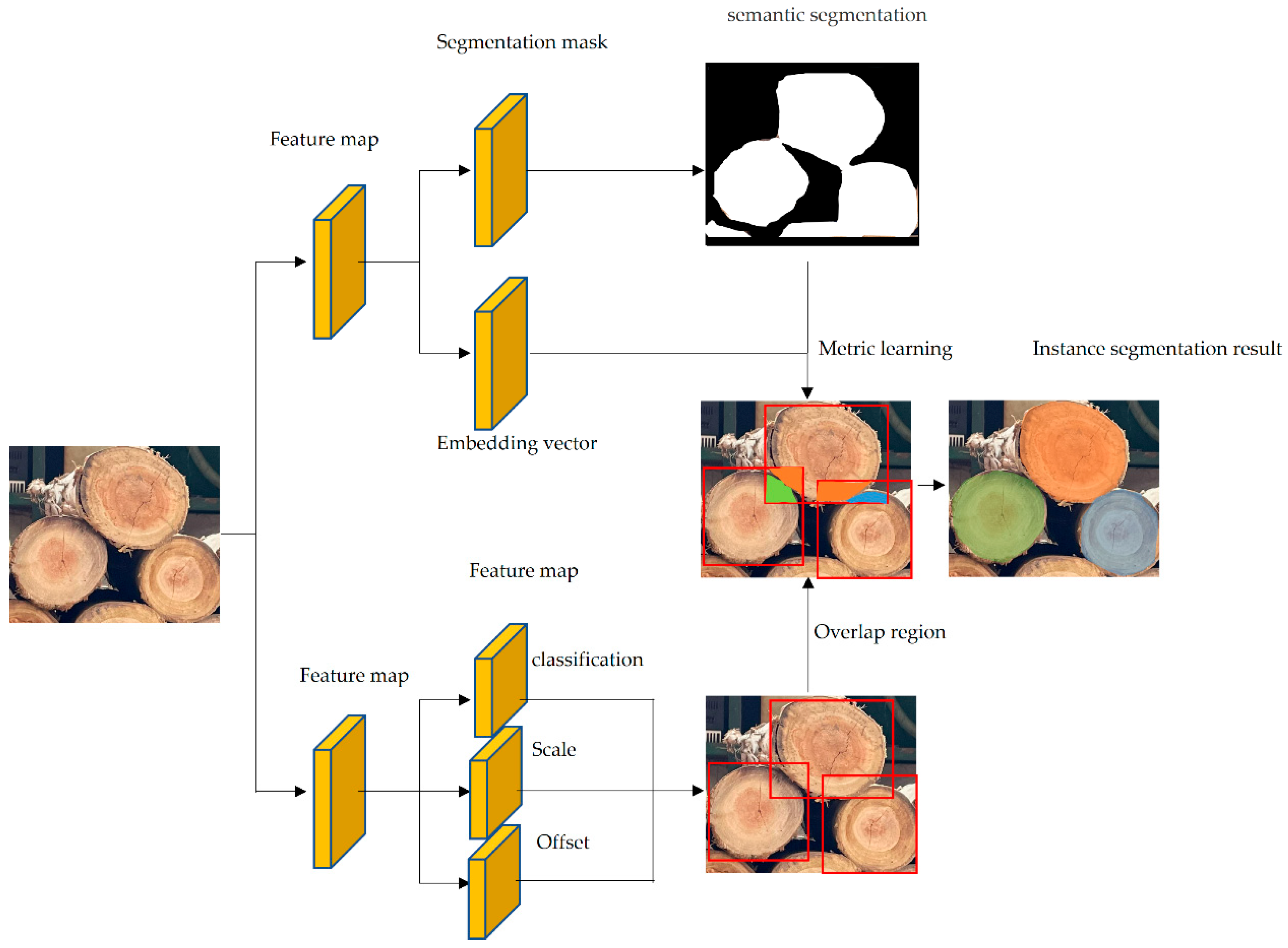
1. Introduction

The forest area in China is 220 million hectares, accounting for 5.4% of the global proportion, or a forest coverage rate of 23% [1]. With the rapid economic development in China, the consumption of forest resources is increasing, in response to which the state has increased its control over the use of forest resources and strictly controlled the transportation of logs through timber inspection [2]. The issue of transportation costs in log logistics transportation is a decisive factor affecting the development of forestry [3]. Therefore, it is of practical significance to improve the efficiency of car-mounted log ruler operations and speed up the transportation process.

Currently, most car-mounted log inspection operations in China are manual inspections, and the operational efficiency needs to be improved. With the development of computer vision technology, it has brought the possibility of automatic measurement of log inspection diameter. Hua Bei [4] extracted the outline of the log end face from the color image by a hole filling algorithm, then fitted the end face outline by Hough circle detection and took the fitted circular diameter as the log end gauge diameter. Cheng-Li [5] implemented on-vehicle log target detection based on the YCbCr and Hough transforms. Yang Pan [6] segmented the detection of logs of each size based on an optimized Mask R-CNN instance segmentation model in a dense stacking scene, and the true detection rate reached 97.99%. Tang Hao [7] first extracted the chromatic aberration features of the image and segmented the features with a clustering algorithm, which could obtain a binary mask of log end faces, thus achieving a recall rate of 91.88%. The development of deep learning has further improved the recall rate of end face extraction. For instance, the SSD model has a 94.87% recall rate for log end face detection [8], YOLOv4 achieves a 93.3% recall rate [9], and the targeted optimized YOLOv3-tiny breaks 98.79%. However, the above traditional image processing algorithms and machine learning processing algorithms need to fine-tune the initial parameters according to different images before detection, and the adjustment of the initial parameters requires expertise in image processing. Therefore, these methods cannot be effectively used in real-world operational scenarios.

Mask-RCNN [10], a method that first performs rectangular frame detection and then traverses the rectangular frame for image segmentation, is also known as the two-stage method. It can be observed that the reason for the inefficiency of the two-stage based instance segmentation method is that the two-stage method requires binary classification (i.e., segmentation) of all pixels within the detection frame. On the one hand, the target box detection and segmentation actions in this method are serial, and each target needs to be detected in order to classify the pixels in the target box. On the other hand, traversing each target frame and classifying all pixels within it increases the invocation overhead of the segmentation model.

In order to improve the performance of the instance segmentation method in the log check path, a fast instance segmentation method based on metric learning is proposed in this paper. As shown in Figure 1, the method extracts the mask image, rectangular box prediction map, and embedding vector map of the image using a convolutional neural network. The mask image is used to extract log end regions, and the rectangular frame prediction image generates an enveloping rectangular frame for each log, which in turn divides the log end regions into instances. For the overlapping regions of the rectangular box, a metric learning paradigm is used to increase the embedding vector distance between pixels located in different logs and decrease the embedding vector distance between pixels of the same log. Finally, the mask pixels of the overlapping regions of the rectangular box are instantiated according to the pixel embedding vectors to obtain the end face mask of each log. The contribution of this paper is summarized as follows:

(1)

Different from mainstream methods like Mask-RCNN, our approach uses a novel parallel architecture for object detection and segmentation, which improves the speed of extracting the end faces of logs.

(2)

By using the metric learning paradigm to distinguish the overlapping areas of adjacent logs, a higher quality of log end face instance segmentation is achieved in this paper.

(3)

In this paper, we use least squares to fit the mask contour, combine it with the true size of the scale to obtain the log ruler diameter, and finally achieve intelligent and fast log ruler diameter measurement.

2. Fast Instance Segmentation Method Based on Metric Learning

2.1. Network Structure of Instance Segmentation Model

The metric learning semantic segmentation method proposed in this paper consists of a backbone network and five model output heads for specific tasks, as exhibited in Figure 2. The backbone convolutional neural network adopts the structure of ResNet50 [11] and is initialized through training on the ImageNet [12] dataset.

The semantic mask regression head is responsible for generating a predictive value for each pixel that represents the probability that the pixel belongs to wood, thus achieving the function of discriminating whether certain regions in the image are wood or not. For the embedding vector regression head, its task is to generate an embedding vector for each pixel, which is used to subsequently distinguish different wood individuals. The three modules, classification header, bounding box regression header, and bounding offset header, are responsible for jointly generating target detection frames that are able to frame different woods and thus roughly segment them. Finally, by performing metric learning, the pixels located within the intersection region of the bounding box will be distinguished according to the embedding vector feature map, and finally the function of instance segmentation is completed.

The proposed model is divided into two parallel branches, which are the detection branch and the segmentation branch. Given an image $I\in R^{w\times h\times 3}$, the detection branch is able to generate three feature maps. They are the center feature map $center\in R^{\frac{w}{4}\times \frac{h}{4}\times 1}$, the scale feature map $scale\in R^{\frac{w}{4}\times \frac{h}{4}\times 2}$, and the offset feature map $offset\in R^{\frac{w}{4}\times \frac{h}{4}\times 2}$. They capture the class of the bounding box, the center position, the box size, and the offset of the object, respectively.

As shown in Figure 2, the detection model generates feature maps with 1/4 of the size of the original image through stacked convolution operations, following the design of CenterNet [13]. This means that each pixel in the feature map represents a 4 × 4 area in the original image. This paper refers to each pixel in the feature map generated by the detection model as a detection point, which is generated uniformly in the original image with a step size of 4 pixels. The value of each detection point can be obtained by $center\in R^{\frac{w}{4}\times \frac{h}{4}\times 1}$. The size of the detection point represents the probability that the point belongs to the center of the log end face. The values in the offset feature map $offset\in R^{\frac{w}{4}\times \frac{h}{4}\times 2}$ represent the displacement vector of each detection point that deviate from the true center position of the log end face. The size of the final detection box can be determined by the scale feature map $scale\in R^{\frac{w}{4}\times \frac{h}{4}\times 2}$, which represents the length and width of the rectangular frame. With the three feature maps generated by the detection branch, the detection boxes of each log end face in the image can be obtained, and thus each log can be detected and distinguished from the others.

For the segmentation branch, given an image $I\in R^{w\times h\times 3}$, it can generate two feature maps. They are the mask map $mask\in R^{w\times h\times 1}$ and the embedding vector map $embedding\in R^{w\times h\times 4}$, respectively. They can be used to obtain the class-level mask of an object and the embedding vector of each pixel. Specifically, the size of any pixel value in the mask map represents the probability of whether the pixel point lies within the log end plane or not. Based on the mask map, a semantic segmentation result for the log end face can then be generated in the image, but it cannot distinguish which log the pixel belongs to. In contrast, each pixel in the embedding vector map stores an embedding vector, which can be used to distinguish different logs and thus finally achieve instance segmentation of log end faces.

2.2. Instance Segmentation Model Loss Function

This section describes the optimization strategies for the detection header and segmentation header, including the center map, scale map, offset map, mask map, and embedding vector map. In addition, there are definitions containing the true labels (center map label, scale map label, offset map label, mask label, and embedding vector label) and loss functions.

The detection branch refers to the well-known model CenterNet [13], which defines three true labels: the classification map label $C\in R^{\frac{w}{4}\times \frac{h}{4}\times 1}$, the scale map label $S\in R^{\frac{w}{4}\times \frac{h}{4}\times 2}$, and the offset map label $O\in R^{\frac{w}{4}\times \frac{h}{4}\times 2}$. These three true labels are used to compare with the center, scale, and offset maps to calculate the model loss, which results in the classification loss of the center feature, the scale loss $L_{scale}$ of the center corresponding detection box, and the offset loss $L_{offset}$ of the bounding box.

To balance the losses, CenterNet adopts weighted loss. Therefore, the total loss of the detection branch is:

$$L_d={\lambda }_{cls}{L}_{cls}+{\lambda }_{scale}{L}_{scale}+{\lambda }_{offset}{L}_{offset}$$

(1)

where ${\lambda }_{cls}$, ${\lambda }_{scale}$, and ${\lambda }_{offset}$ are the weights of the three losses.

The semantic segmentation branch loss function refers to the well-known model SFnet [14], which defines the mask label $M_{ask}\in R^{w\times h\times c}$ to calculate the loss between the segmentation mask and the true segmentation label. In comparison with SFnet, this paper adds a branch to predict the embedding vector of pixels, which is obtained by optimization through metric learning. The loss function of the semantic segmentation branch is shown as follows:

$$L_{seg}={\lambda }_{mask}{L}_{mask}+{\lambda }_{inst}{L}_{inst}$$

(2)

where $L_{seg}$ is the total loss function of the segmentation branch, ${\lambda }_{mask}$ and $L_{inst}$ are the weights of each loss. $L_{mask}$ is the difference between the segmentation mask and the true segmentation label, and its specific details can be found in the original SFnet paper. $L_{inst}$ is the loss of the embedding vector, which will be highlighted in the subsequent sections of this paper. The loss function of the entire model is:

$$L_{total}=L_d+L_{seg}$$

(3)

2.3. Metric Learning Representation

Conventional object detection and semantic segmentation can get the bounding box and mask image of an object. The mask obtained by semantic segmentation is specific to a category and cannot distinguish individual instances (e.g., it can identify the end faces of logs in a whole image but cannot effectively distinguish each individual log). In this paper, we add a branch to the head of semantic segmentation, which produces an embedding vector for each pixel in the image. In this paper, all pixels from each instance are considered to be of the same class, while pixels from different instances are of different classes. Then, metric learning is applied to optimize intra-class compactness and inter-class differences. When applying metric learning to optimize the embedding vectors of all pixels, a large amount of computational resources are required. Three pieces of prior knowledge can be obtained based on the bounding box and mask of an instance. (1). The mask of an instance is in the bounding box. (2). If the bounding box of an instance does not intersect the bounding boxes of other instances, the mask in the bounding box is the mask of that instance. (3). If the bounding box of an instance intersects the bounding boxes of other instances, it is necessary to determine from which instance the mask of the intersecting region comes. Therefore, only the pixels of the intersection region need to be optimized by metric learning, which greatly reduces the computational resources.

Based on the above part, the embedding vector of each pixel in the intersection region needs to be optimized. The implementation steps are as follows: there are many instances in a picture, and each instance is treated as an anchor instance. If there is an intersection region between the bounding boxes of an anchor instance and the bounding box of another instance, an instance pair $\left\{I_i,O_{ij}\right\}$ is formed. Here, $I_i$ represents the i-th anchor instance, and $O_{ij}$ represents the j-th instance whose bounding box intersects with the i-th anchor instance. Through the above calculation, all instance pairs in an image can be obtained and represented as follows: $\left\{I_1,O_{11}\right\}$, $\left\{I_1,O_{12}\right\}$, …, $\left\{I_2,O_{21}\right\}$, $\left\{I_2,O_{22}\right\}$, …, $\left\{I_i,O_{ij}\right\}$, …, $\left\{I_i,O_{ij}\right\}$. Taking $\left\{I_i,O_{ij}\right\}$ as an example, if the pixels belong to the instance pairs and lie in the intersection region, the embedding vectors of these pixels need to be optimized. In this paper, we propose the following optimization strategy: 1. The embedding vectors of the centroids of the instance pairs $\left\{I_i,O_{ij}\right\}$ are defined as $e_I$ and $e_O$, respectively. If a pixel is in the intersection area $\left\{I_i,O_{ij}\right\}$ and belongs to instance $I_i$, its embedding vector is defined as $e_{I,i}$. If the pixel in $\left\{I_i,O_{ij}\right\}$ belongs to $O_{ij}$, it is defined as $e_{O,i}$. 2. The optimization of the embedding vector is divided into two parts. In the first part, $e_{I,i}$ is made closer to $e_I$ while being farther away from $e_O$. Similarly, in the second part, $e_{O,i}$ is made closer to $e_O$ while being farther away from $e_I$. In summary, the function can be written as:

$$L_{ij}^1=\left\{\begin{array}{cc}\hfill \frac{1}{N}{\displaystyle \sum _{i=1}^N}\max \left(0,\Phi +{\left|e_I-e_{I,i}\right|}_2^2-{\left|e_O-e_{I,i}\right|}_2^2\right),& N>0\hfill \\ \hfill 0,& \mathrm{else}\hfill \end{array}\right.$$

(4)

$$L_{ij}^2=\left\{\begin{array}{cc}\hfill \frac{1}{M}{\displaystyle \sum _{i=1}^M}\max \left(0,\Phi +{\left|e_O-e_{O,i}\right|}_2^2-{\left|e_I-e_{O,i}\right|}_2^2\right),& M>0\hfill \\ \hfill 0,& \mathrm{else}\hfill \end{array}\right.$$

(5)

where $L_{ij}^1$ represents the loss of instance $I_i$, and $L_{ij}^2$ represents the loss of instance $O_{ij}$. N refers to the number of pixels belonging to instance $I_i$ and in the intersection area $\left\{I_i,O_{ij}\right\}$, while M refers to the number of pixels belonging to an instance $O_{ij}$ and in the intersection area $\left\{I_i,O_{ij}\right\}$. $\Phi$ is the hyperparameter, which is set here to 0.5. By using the above method, the loss $L_P=L_{ij}^1+L_{ij}^2$ is achieved. Since $L_P$ here represents the loss of $\left\{I_i,O_{ij}\right\}$, thereby the losses of all instance pairs need to be summed up. However, when an image has a large number of instance pairs, there may be many embedding vectors to be optimized, which requires a large amount of computational resources. Therefore, a random sampling method is designed to randomly select a few instance pairs from the image to calculate the loss. The unselected instance pairs are not involved in the loss calculation. The above method greatly reduces the demand on computational resources. The designed loss function is as follows:

$$L_{inst}=\left\{\begin{array}{cc}\hfill \frac{1}{K}{\displaystyle \sum _{i=1}^K}{\mathrm{r}\mathrm{a}\mathrm{n}\mathrm{d}\mathrm{o}\mathrm{m}}_i\left(L_P\right),& P>K\hfill \\ \hfill \frac{1}{P}{\displaystyle \sum _{p=1}^P}{L}_P,& \mathrm{else}\hfill \end{array}\right.$$

(6)

where $L_{inst}$ is the final metric loss, K is set to represent randomly selecting K instance pairs for calculation in this paper.

2.4. Training Methods for Instance Segmentation Models

In order to train and validate the instance segmentation model, the collection and labeling of the end-face instance segmentation dataset are required. The experimental data were collected from Gaofeng Forest Farm in Xixiangtang District, Nanning, Guangxi, using a Huawei P30 as the image acquisition device. A total of 1000 operational images were collected for this paper by shooting at different distances for different operational piles (which were able to obtain log end faces with different shapes and sizes). In addition, the Labelme image annotation software was used to annotate the log ends in the images with contours, and the original images and the annotated JSON files were batch processed to generate a dataset, which was divided into training, validation, and test sets in the ratio of 8:1:1.

In this paper, the average precision (AP) of segmentation masks was utilized as the evaluation metric for the model’s performance.

$$\mathrm{A}\mathrm{P}=\sum _{i=1}^n\frac{1}{n}\times \frac{\mathrm{T}\mathrm{P}}{\mathrm{T}\mathrm{P}+\mathrm{F}\mathrm{P}}$$

(7)

For $I_i$, true positive $\left(\mathrm{T}\mathrm{P}\right)$ represents the number of pixels correctly segmented, and a false positive $\left(\mathrm{F}\mathrm{P}\right)$ represents the number of pixels wrongly predicted to belong to that instance. Additionally, $n$ denotes the number of instances in the dataset. The model’s segmentation accuracy on logs of different sizes was measured using scale-related $\mathrm{AP}$ values of $\mathrm{A}{\mathrm{P}}_{\mathrm{l}\mathrm{a}\mathrm{r}\mathrm{g}\mathrm{e}}$, $\mathrm{A}{\mathrm{P}}_{\mathrm{m}\mathrm{i}\mathrm{d}}$, and $\mathrm{A}{\mathrm{P}}_{\mathrm{s}\mathrm{m}\mathrm{a}\mathrm{l}\mathrm{l}}$ to validate the segmentation accuracy of the model on instances of different sizes. All instances in the dataset were sorted based on their actual end-face sizes to divide the instances into $large$, $mid$, and $small$ categories.

Furthermore, the model’s frames per second (FPS) on a Windows system with an i7 chip and an NVIDIA GTX1060 graphics card was used as the performance metric in this paper to demonstrate the model’s inference speed.

2.5. Application of Proposed Instance Segmentation Model for Log End Detection

The proposed fast log end-face instance segmentation technique based on metric learning can be used in real-world operational scenarios. In order to verify the size-checking performance of the diameter, images were all taken of eucalyptus logs of three different sizes (large: log ruler diameter above 14 cm, medium: log ruler diameter between 10 cm and 14 cm, small: log ruler diameter between 6 cm and 10 cm) at Gaofeng Forest Farm, Xixiangtang District, Nanning, Guangxi. Each log was checked by professional workers to get the true value for comparison and analysis. The images were collected with a Huawei P30 smartphone between 2 p.m. and 3 p.m. Before image collection, the logs were loaded onto a truck to make the experimental scene closer to the real operational scenario.

To make the model applicable to the log ruler inspection operation. First, the images were segmented by instances to get the end face mask of each log, and the edge contour of the log end face was extracted by a convex wrapping algorithm. Then, in order to get the scaling ratio between the real world and the image, the inner diameter of the truck’s rear wheel was selected as a reference, and the scaling factor was calculated based on its real length and its length in the image. Finally, in order to meet the operational criteria of the actual check-rule operation, the log end face was fitted using the least-squares ellipse fitting principle. First, the coordinate points of the edge contour are calculated according to the log end face mask image then, the contour center coordinates are derived according to the form center calculation formula, and finally, the ellipse minimized with the boundary coordinate distance metric is found according to the Euclidean distance formula. The actual diameter of the log was obtained by multiplying the length of the minor axis of the ellipse by the scaling factor of the image.

3. Results and Analysis of the Instance Segmentation Model

Results of Log End-Face Mask Extraction Using Instance Segmentation Model

The parameters involved in this paper primarily comprise the weights of various loss functions, ${\lambda }_{cls}$, ${\lambda }_{scale}$, ${\lambda }_{offset}$, ${\lambda }_{mask}$, ${\lambda }_{inst}$, and the number of randomly selected instance pairs, $K$, in metric learning. In this paper, ${\lambda }_{cls}+{\lambda }_{scale}+{\lambda }_{offset}=1$, and ${\lambda }_{mask}+{\lambda }_{inst}=1$. Concerning the weights used in the loss functions, a brute force approach was adopted to search for the optimal combination of weights by continuously trying different weight values to achieve the best performance of the model on the validation set. The top five parameter combinations for the AP values on the test set are listed in

Table 1. Performance Comparison of Loss Function Weights.

${\mathit{\lambda }}_{\mathit{c}\mathit{l}\mathit{s}}$	${\mathit{\lambda }}_{\mathit{s}\mathit{c}\mathit{a}\mathit{l}\mathit{e}}$	${\mathit{\lambda }}_{\mathit{o}\mathit{f}\mathit{f}\mathit{s}\mathit{e}\mathit{t}}$	${\mathit{\lambda }}_{\mathit{m}\mathit{a}\mathit{s}\mathit{k}}$	${\mathit{\lambda }}_{\mathit{i}\mathit{n}\mathit{s}\mathit{t}}$	$\mathbf{A}\mathbf{P}$
0.3	0.4	0.3	0.5	0.5	0.912
0.2	0.5	0.3	0.4	0.6	0.910
0.4	0.3	0.3	0.5	0.5	0899
0.5	0.3	0.2	0.6	0.4	0.897
0.2	0.3	0.5	0.3	0.7	0.896

.

This study revealed that a larger K (the number of randomly collected instance pairs in metric learning) led to better model performance but at the cost of significantly slower training speed. Besides, the training speeds under different K values (100 epochs of iteration) were compared, and the experimental results are provided in

Table 2. Training Time for 200 Epochs Under Different K Values.

K	Training Time	$\mathbf{A}\mathbf{P}$
1	32 min	0.902
3	56 min	0.905
3	1 h 20 min	0.912
4	2 h 50 min	0.913
5	5 h 12 min	0.925

:

When K was set to 3, a relatively good value of AP was achieved without excessively long training time. Subsequent experiments were conducted based on the parameters in the first row of Table 1, and K = 3. The iteration curve of the loss function is illustrated in Figure 3.

The proposed model was compared with several well-known models, including Mask-RCNN, FCIS [15], MEinst [16], PersonLab [17], EmbedMask [18], and SparseInst [19], to validate its performance. The experimental results are presented in

Table 3. Comparison of Overall Performance of Different Models.

Models	$\mathbf{A}\mathbf{P}$	${\mathbf{A}\mathbf{P}}_{\mathbf{l}\mathbf{a}\mathbf{r}\mathbf{g}\mathbf{e}}$	${\mathbf{A}\mathbf{P}}_{\mathbf{m}\mathbf{i}\mathbf{d}}$	${\mathbf{A}\mathbf{P}}_{\mathbf{s}\mathbf{m}\mathbf{a}\mathbf{l}\mathbf{l}}$	FPS
Mask-RCNN	0.842	0.878	0.838	0.810	8.6
FCIS	0.827	0.848	0.831	0.803	8.1
MEinst	0.835	0.852	0.835	0.820	4.2
PersonLab	0.818	0.844	0.821	0.791	24.7
EmbedMask	0.864	0.881	0.862	0.851	16.7
SparseInst	0.714	0.810	0.579	0.753	44.6
Our	0.912	0.912	0.911	0.913	50.2

.

The experimental results show that the proposed model has a faster processing speed and a higher segmentation accuracy. In addition, Table 3 shows that the segmentation accuracy of the comparison method decreases as the scale of the target instances decreases. However, as shown in the fifth column of Table 3, the proposed model can segment log end faces of smaller scales better. Therefore, it can be seen that the proposed model can be more flexible, automated, and intelligent in its actual production.

The analysis of the visualization results can more intuitively demonstrate the advantages of the proposed method. Figure 4 shows the segmentation results of the proposed algorithm model. As shown in the figure, the proposed method can effectively deal with the situation where the logs are masked to each other during the shooting process, as can be seen in this paper where the orange corresponding logs mask part of the blue logs. In the second column, the third column, Mask-RCNN and EmbedMask, cannot handle the occlusion situation properly, and the model will recognize the orange logs as blue logs, which cannot handle the occlusion situation well.

4. Model Detection Diameter Results and Analysis

To verify the effectiveness of the proposed model, it was compared with Mask-RCNN and EmbedMask for the effect of log ruler diameter detection performance. As shown in

Table 4. Model Performance Comparison.

Model	Mean Relative Error/%	Standard Deviation/%	Frame Rate/FPS
Mask-RCNN	−5.13	5.81	8.6
EmbedMask	−5.09	5.78	16.7
Ours	−4.62	5.16	50.2

, an analysis of the detected dimensions of the model with the true values can be obtained. The average relative error of the proposed model is −4.62% and the standard deviation is 5.16%. Mask-RCNN has an average relative error of −5.13% and a standard deviation of 5.81%. EmbedMask has an average relative error and standard deviation of −5.09% and 5.78%, respectively. In terms of processing speed, the proposed model’s processing speed is about three times faster than that of EmbedMask and about five times faster than that of Mask-RCNN. Figure 5 shows the performance of the model in vehicular scenarios in this paper.

To verify the effect of shooting distance on the performance of the model, front-facing images were captured at distances of 1 m, 2 m, 3 m, 4 m, and 5 m from the transport vehicle.

Table 5. Average Diameter Measurement Error at Various Distances.

Distance/m	Mean Absolute Error/mm	Mean Relative Error/%
1	−4.13	−4.81
2	−4.09	−4.78
3	−4.01	−4.62
4	−5.40	−6.18
5	−8.79	−8.14

shows the average diameter measurement error of the model at different distances. As seen from Table 5, the error does not vary much when the acquisition distance is 0~3 m. The average absolute errors are all less than −4.13 mm, and the average relative errors are all less than −4.81%. As can be seen from Table 5, when the shooting distance is less than 3 m, the measurement error slightly increases. We suspect that this is caused by uneven focusing due to the close distance. When the distance becomes larger, the error increases significantly. When the capture distance is 5 m, the average absolute error reaches −8.79 mm, and the average relative error reaches −8.14%. As the distance increases, the number of pixels on the end face of each log in the image decreases significantly, which increases the segmentation difficulty of the example segmentation model and therefore the error increases significantly. Finally, it can be seen from Table 5 that the best results for the check-rule diameter are obtained when the acquisition distance is 3 m. The average absolute error and the average relative error at this time are −4.01 mm and −4.62%, respectively.

To verify the influence of different shooting heights on the model’s performance, we conducted frontal shootings of the transport vehicle at heights of 1.6 m, 1.8 m, 2.0 m, and 2.2 m, respectively. Photographs of the end surfaces were taken at distances of 3 m from the transport vehicle.

Table 6. Average Diameter Measurement Error at Various Distances.

Height/m	Mean Absolute Error/mm	Mean Relative Error/%
1.6	−4.01	−4.62
1.8	−3.98	−4.60
2.0	−4.04	−4.63
2.2	−4.06	−4.64

shows the average diameter measurement error of the model at different shooting heights. From Table 6, we can observe that the performance is fairly consistent across the different shooting heights, with the average absolute error ranging from −4.01 mm to −4.06 mm and the average relative error ranging from −4.60% to −4.64%. This suggests that the model is robust to changes in shooting height and can make accurate predictions regardless of the height at which the images are taken. However, it has been observed that the model performs at its best when the shooting height is 1.8 m. The analysis presented in this paper suggests that this is due to the fact that as the shooting position approaches the center of gravity of the log pile, the image quality improves significantly. Moreover, capturing images at the height of the load center reduces the overlap error.

To further investigate the performance of the model under different scenarios, photographs of the end surfaces were taken at distances of 3 m from the transport vehicle in seven different positions: head-on, leftward at 10, 20, and 30 degrees, and rightward at 10, 20, and 30 degrees.

Table 7. Average Diameter Measurement Error at Different Viewing Angles.

Angle	Mean Absolute Error/mm	Mean Relative Error/%
30 degrees to the left	−12.51	−13.98
20 degrees to the left	−9.49	−10.83
10 degrees to the left	−5.21	−6.35
Is on	−4.01	−4.62
10 degrees to the right	−5.23	−6.36
20 degrees to the right	−9.53	−10.85
30 degrees to the right	−12.79	−14.02

shows the average diameter measurement error of the model at different angles. It can be seen that different viewing angles caused different degrees of influence on the model’s performance. When the viewing angle deviates from the direction of the front-to-side end face, the accuracy of the ruler diameter check decreases. The average absolute error and the average relative error are the largest when the shooting viewpoint deviates from the orthogonal end direction by 30 degrees, which are −12.79 mm and −14.02%, respectively. The relationship between the degree of deviation from the head-on direction and the size of the error shows that the further the shooting angle is deviated from the right direction, the larger the error is. As shown above, the method of checking the diameter of the logs based on the example segmentation requires a high degree of head-on alignment during data collection of the end face of the log.

In this paper, volume measurement of logs was further carried out using volume measurement standards of different countries based on the results of the check-measure diameter. In this paper, Chinese, American, Russian, and Japanese standards were selected for volume measurement. The Russian measurement standard is the look-up table method, and the other three countries use a formula calculation method. Since the volume calculation of logs requires knowledge of the length of the log ruler, and since the local timber collection operation in Guangxi is conducted at a fixed length, with each log segment having a fixed length of 1.27 m, this study used 1.27 m as the final measuring length.

Table 8. Comparison of Volume Calculations Using Standards from Different Countries.

Nation	Method	True Volume/m3	Measure Volume/m3	Error/%
China	$V=0.8L{\left(D+0.5L\right)}^2÷\mathrm{10,000}$	4.87	4.66	−4.25
Russia	none	4.63	4.39	−5.02
The U.S.	$V=\frac{\left(D^2-3D\right)L}{5}$	5.32	4.98	−6.32
Japan	$V=\frac{D^{2}L}{\mathrm{10,000}}$	4.28	4.03	−5.73

shows the volume calculation errors of the model using standards from different countries. It can be seen that the model has the smallest error of 4.25% in volume measurement under the Chinese standard. Due to the use of English units in the US standard and the fact that the gradation of the ruler diameter differs greatly from other countries, the largest error was observed when using the US standard. In summary, the model proposed in this study for log ruler application has high accuracy and detection speed.

5. Conclusions

The bottleneck of the existing instance segmentation-based log end face inspection ruler diameter technique is its low computational speed. Therefore, a fast instance segmentation technique for log end face detection and semantic segmentation based on metric learning is proposed to parallelize the semantic segmentation of target detection. Unlike existing instance segmentation methods, the proposed method is able to perform end face detection and semantic segmentation of images in parallel. Since semantic segmentation of the entire image would confuse the adjacent log end faces, this paper proposes a metric learning-based instance segmentation algorithm that reclassifies the pixels in the overlapping area according to the metric learning framework and thus achieves fast instance segmentation. By comparing with existing methods, the proposed fast instance segmentation method is able to improve the accuracy by 7% while simultaneously increasing the inference speed by 43 FPS.

The proposed instance segmentation method can be effectively applied to the log ruler diameter measurement. The experimental results show that the computational error of the proposed model is −4.62% for the log check gauge, which is more accurate than the existing methods. By varying the distance and angle, the measurement of the pile of logs was found to have the smallest error of −4.01 mm when the model was measured at a distance of 3 m and facing the end of the log. In addition, the volume measurement error calculated by the proposed model according to the domestic volume calculation standard is −4.25%, which fully demonstrates the practicality of the proposed method.

The proposed model is expected to improve the efficiency of timber measurement and potentially reduce the transportation cost of timber. This article presents opportunities for further research. Specifically, the performance of the model was observed to decrease significantly when the shooting distance was too far or the shooting angle was tilted. We have considered that the main reasons for the performance degradation of the model in the above-mentioned scenarios are difficulties in detecting small and densely packed targets. In future work, we will draw on small object detection models [20,21,22,23,24] and dense object detection models [25,26,27,28,29] to further improve this paper. Additionally, exploring how to apply the model to other modalities, such as thermal imaging [30], is an important research direction to pursue.

References

- National Bureau of Statistics of China. China Statistical Yearbook (2020); China Statistics Press: Beijing, China, 2020. [Google Scholar]
- Jiang, W. Lumber Inspection and Its Importance in Lumber Shipping Inspection. Jiangxi Agric. 2019, 4, 92–93. [Google Scholar]
- Li, M. Research on Optimal Algorithm of Logistics System for Timber Transportation in Forest Area; Beijing Forestry University: Beijing, China, 2016. [Google Scholar]
- Hua, B.; Cao, P.; Huang, R.W. Research on log volume detection method based on computer vision. J. Henan Inst. Sci. Technol. Nat. Sci. Ed. 2022, 50, 64–69. [Google Scholar]
- Chen, G.H.; Zhang, Q.; Chen, M.Q.; Li, J.W.; Yin, H.Y. Log diameter-level fast detection algorithm based on binocular vision. J. Beijing Jiaotong Univ. 2018, 42, 9. [Google Scholar]
- Keck, C.; Schoedel, R. Reference Measurement of Roundwood by Fringe Projection. For. Prod. J. 2021, 71, 352–361. [Google Scholar] [CrossRef]
- Tang, H.; Wang, K.J.; Li, X.Y.; Jian, W.H.; Gu, J.C. Detection and statistics of log image end face based on color difference clustering. China J. Econom. 2020, 41, 7. [Google Scholar]
- Tang, H.; Wang, K.; Gu, J.C.; Li, X.; Jian, W. Application of SSD framework model in detection of logs end. J. Phys. Conf. Ser. 2020, 1486, 072051. [Google Scholar] [CrossRef]
- Cai, R.X.; Lin, P.J.; Lin, Y.H.; Yu, P.P. Bundled log end face detection algorithm based on improved YOLOv4-Tiny. Telev. Technol. 2021, 45, 9. [Google Scholar]
- He, K.; Gkioxari, G.; Dollár, P.; Girshick, R. Mask r-cnn. In Proceedings of the IEEE International Conference on Computer Vision, Honolulu, HI, USA, 21–26 July 2017; pp. 2961–2969. [Google Scholar]
- He, K.; Zhang, X.; Ren, S.; Sun, J. Deep Residual Learning for Image Recognition. In Proceedings of the 2016 IEEE Conference on Computer Vision and Pattern Recognition (CVPR), Las Vegas, NV, USA, 27–30 June 2016. [Google Scholar]
- Simonyan, K.; Zisserman, A. Very deep convolutional networks for large-scale image recognition. arXiv 2014, arXiv:1409.1556. [Google Scholar]
- Zhou, X.; Wang, D.; Krähenbühl, P. Objects as points. arXiv 2019, arXiv:1904.07850. [Google Scholar]
- Li, X.; You, A.; Zhu, Z.; Zhao, H.; Yang, M.; Yang, K.; Tan, S.; Tong, Y. Semantic flow for fast and accurate scene parsing. In Proceedings of the European Conference on Computer Vision, Glasgow, UK, 23–28 August 2020; Springer: Cham, Switzerland, 2020; pp. 775–793. [Google Scholar]
- Li, Y.; Qi, H.; Dai, J.; Ji, X.; Wei, Y. Fully convolutional instance-aware semantic segmentation. In Proceedings of the IEEE Conference on Computer Vision and Pattern Recognition, Honolulu, HI, USA, 21–26 July 2017; pp. 2359–2367. [Google Scholar]
- Zhang, R.; Tian, Z.; Shen, C.; You, M.; Yan, Y. Mask encoding for single shot instance segmentation. In Proceedings of the IEEE/CVF Conference on Computer Vision and Pattern Recognition, Seattle, WA, USA, 14–19 June 2020; pp. 10226–10235. [Google Scholar]
- Papandreou, G.; Zhu, T.; Chen, L.C.; Gidaris, S.; Tompson, J.; Murphy, K. Personlab: Person pose estimation and instance segmentation with a bottom-up, part-based, geometric embedding model. In Proceedings of the European Conference on Computer Vision (ECCV), Munich, Germany, 8–14 September 2018; pp. 269–286. [Google Scholar]
- Ying, H.; Huang, Z.; Liu, S.; Shao, T.; Zhou, K. Embedmask: Embedding coupling for one-stage instance segmentation. arXiv 2019, arXiv:1912.01954. [Google Scholar]
- Cheng, T.; Wang, X.; Chen, S.; Zhang, W.; Zhang, Q.; Huang, C.; Liu, W. Sparse Instance Activation for Real-Time Instance Segmentation. In Proceedings of the IEEE/CVF Conference on Computer Vision and Pattern Recognition, New Orleans, LA, USA, 18–24 June 2022; pp. 4433–4442. [Google Scholar]
- Liu, Y.; Sun, P.; Wergeles, N.; Shang, Y. A survey and performance evaluation of deep learning methods for small object detection. Expert Syst. Appl. 2021, 172, 114602. [Google Scholar] [CrossRef]
- Lim, J.S.; Astrid, M.; Yoon, H.J.; Lee, S.I. Small object detection using context and attention. In Proceedings of the 2021 International Conference on Artificial Intelligence in Information and Communication (ICAIIC), Jeju Island, Republic of Korea, 13–16 April 2021; pp. 181–186. [Google Scholar]
- Bosquet, B.; Mucientes, M.; Brea, V.M. STDnet-ST: Spatio-temporal ConvNet for small object detection. Pattern Recognit. 2021, 116, 107929. [Google Scholar] [CrossRef]
- Leng, J.; Ren, Y.; Jiang, W.; Sun, X.; Wang, Y. Realize your surroundings: Exploiting context information for small object detection. Neurocomputing 2021, 433, 287–299. [Google Scholar] [CrossRef]
- Liu, M.; Wang, X.; Zhou, A.; Fu, X.; Ma, Y.; Piao, C. Uav-yolo: Small object detection on unmanned aerial vehicle perspective. Sensors 2020, 20, 2238. [Google Scholar] [CrossRef] [PubMed] [Green Version]
- Zhang, H.; Wang, Y.; Dayoub, F.; Sunderhauf, N. Varifocalnet: An iou-aware dense object detector. In Proceedings of the IEEE/CVF Conference on Computer Vision and Pattern Recognition, Nashville, TN, USA, 20–25 June 2021; pp. 8514–8523. [Google Scholar]
- Qiu, H.; Ma, Y.; Li, Z.; Liu, S.; Sun, J. Borderdet: Border feature for dense object detection. In Proceedings of the Computer Vision—ECCV 2020: 16th European Conference, Glasgow, UK, 23–28 August 2020; Part I 16. Springer International Publishing: Berlin/Heidelberg, Germany, 2020; pp. 549–564. [Google Scholar]
- Chen, Z.; Yang, C.; Li, Q.; Zhao, F.; Zha, Z.J.; Wu, F. Disentangle your dense object detector. In Proceedings of the 29th ACM International Conference on Multimedia, New York, NY, USA, 20–24 October 2021; pp. 4939–4948. [Google Scholar]
- Zhu, B.; Wang, J.; Jiang, Z.; Zong, F.; Liu, S.; Li, Z.; Sun, J. Autoassign: Differentiable label assignment for dense object detection. arXiv 2020, arXiv:2007.03496. [Google Scholar]
- Gao, Z.; Wang, L.; Wu, G. Mutual supervision for dense object detection. In Proceedings of the IEEE/CVF International Conference on Computer Vision, Montreal, BC, Canada, 11–17 October 2021; pp. 3641–3650. [Google Scholar]
- Glowacz, A. Thermographic fault diagnosis of electrical faults of commutator and induction motors. Eng. Appl. Artif. Intell. 2023, 121, 105962. [Google Scholar] [CrossRef]