Abstract
The correlation between climate change and pine tree dieback must be understood to implement a proactive forest management system. In this study, an ensemble model combining random forest, the generalized boosting model, and the generalized linear model was used to analyze the topographical and environmental characteristics of pine trees suffering from dieback in the Wangpicheon Ecosystem and Landscape Conservation Area, and the areas in which pine trees are at risk of dieback were evaluated to promote efficient pine forest management. The results showed that pine trees suffering from dieback in the conservation area were mainly located on ridges, were age class 6 or older, or were in areas with a low topographic wetness index south of the conservation area. An evaluation of the risk of dieback among pine trees was performed based on the results of two ensemble models. An area of 365 ha accounting for 6.8% of the total area was identified as requiring “caution” with respect to the risk of dieback of coniferous forests and mixed forests. The developed methodology is expected to provide valuable information for the implementation of an appropriate management system for the protection of pine and mixed forests from the negative effects of climate change.
1. Introduction
Korean red pine (Pinus densiflora Siebold & Zucc.) is widely distributed across the Korean Peninsula, Shandong Province, China, Japan, and Manchuria [1]. It typically grows on rocky outcrops, weathered rocks, mountain peaks, and fertile soils [2]. In addition, compared to other tree species, Pinus densiflora has a high adaptability to dry environments and has high ecological and economic value [3]. With these characteristics, pine trees are called indigenous species of temperate coniferous forests in East Asia, and research on this species is continuing steadily.
Temperatures have rapidly increased over the past decade, and mid-latitude regions have shown greater increases compared to other regions [4,5]. Predicting the impact of climate change on vegetation distribution is an important research topic globally [6,7,8]. Temperature increases can shift the boundaries of the ranges of species and alter biodiversity, ecosystem structure, and function [9,10], and accordingly, changes in the distribution of pine trees have been reported [11,12].
In Korea, pine tree forests account for approximately 26% of the total forest plantation area [13], and their protection contributes to the coexistence of coniferous and broad-leaved trees and the formation of “mixed forests,” which are considered important factors in promoting biodiversity [13]. However, recent reports on the damage to pine tree forests in various areas, such as the Wangpicheon Ecosystem and Landscape Conservation Area (ELCA), the Sogwang-ri Forest Genetic Resources Reserve, and the Mt. Odae and Mt. Seorak areas in Gangwon-do, have indicated that pine tree habitats on the Korean Peninsula are increasingly threatened. High temperatures and dryness during a specific period and extreme drought conditions in autumn and winter are considered to be the causes [14].
Therefore, it is necessary to investigate the correlation between climate change factors and pine tree dieback, and establish a proactive forest management system based on the generation of continuous information to develop forest management measures [15]. To achieve this, it is necessary to gather accurate information on the environmental conditions of the dieback pine trees, as well as to prioritize the selection of investigation sites. In this regard, a species distribution model (SDM) [16,17,18,19], which is a biological species habitat prediction model, was utilized, and an ensemble model combining statistical and machine learning models was applied to reduce the uncertainty of a single model [20]. Ensemble modeling has the advantage of compensating for result uncertainty by preventing divergent prediction outcomes within a single species distribution model caused by different algorithms [21].
The objectives of this study were to analyze the topographical and forest stand characteristics of dieback areas and understand the relationship between the location characteristics of pine trees in dieback areas and weather factors. Specifically, we aimed to (1) compare the characteristics of dieback pine trees and growth areas by considering various environmental factors and forest stand characteristics and (2) develop a model that can evaluate pine tree dieback risk areas using an ensemble model that combines individual SDMs. The results of our study are expected to serve as a reference to evolve policy measures and implement an appropriate management system for the protection of pine and mixed forests from the negative effects of climate change.
2. Materials and Methods
2.1. Study Site
The study area focuses on the Wangpicheon ELCA in Uljin, which corresponds to the administrative districts of Geumgangsong-myeon, Geunnam-myeon, and Subi-myeon in Uljin-gun, Gyeongsangbuk-do. It is classified into a 45.35 km2 core area, a 55.64 km2 buffer area, and a 1.85 km2 transition area according to ecological and landscape functions (Figure 1). Most forests in this area consist of Pinus densiflora f. erecta, which is highly valued for conservation in the Uljin and Bonghwa regions [22].
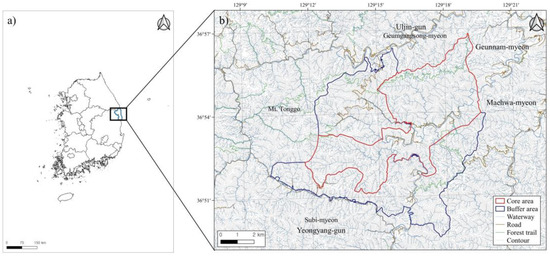
Figure 1.
(a) Uljin-gun area on the Korean peninsula. (b) Map of the study site: Wangpicheon Ecological Landscape Conservation Area.
2.2. Sampling in Areas of Pine Tree Dieback/Growth
A 2-year remote sensing study was conducted in the Wangpicheon ELCA from 2021 to 2022. Remote sensing images were captured in November–December 2021 and from May to July 2022 to distinguish dieback pine trees. Additionally, we took photographs from multiple angles to minimize the effect of shading caused by topographical factors and improve the accuracy of identifying dead pine trees. Using the acquired orthophotos, we utilized information such as color and shape to identify dieback pine trees. In the orthophoto images, dead pine trees can be distinguished from other tree species by their unique branching pattern, which spreads out like a star. We extracted dead pine trees based on the characteristic of leaves falling off and revealing only white branches in dieback pine trees [15]. To confirm the identification of dieback pine trees, a 50 cm pixel size resolution was used. Based on the acquired orthophotos, we extracted the areas where the death of pine trees occurred in the collective dieback. In 2022, nine areas exhibiting collective dieback were identified through an on-site investigation based on remote sensing observations. This study involved a comprehensive survey based on both remote sensing and on-site investigations within the conservation area; however, the analysis was limited to coniferous and mixed forests dominated by Pinus densiflora. Only eight of the nine areas exhibiting collective dieback were located within the coniferous and mixed forests and were, therefore, used for the analysis. To accurately analyze the topographic and environmental characteristics of pine trees exhibiting dieback and to evaluate the areas at risk of such dieback, dieback pine tree samples were classified into areas with collective dieback and individual tree dieback based on on-site confirmation, and these were then analyzed separately. Collective dieback sites were defined as cases where four or more pine trees in close proximity exhibited dieback; “proximity” was defined as a distance of up to 30 m between the centers of the four trees exhibiting a collective dieback, as determined from orthophotos (Figure 2). Quadrats were installed at locations where collective dieback sites were found, and different quadrat sizes of 20 × 20 m and 20 × 10 m were used, considering the topographic characteristics and number of dieback trees.
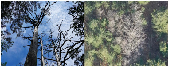
Figure 2.
Trees suffering collective dieback.
To avoid the spatial autocorrelation of occurrence points due to sampling bias, samples were extracted from the collective dieback area points and individual dieback points by removing duplicate points to ensure that each grid cell was represented by one occurrence point for environmental variables [23,24,25,26,27,28]. As a result, there were 35 samples from the collective dieback area points and 105 samples from individual dieback points. In addition, areas where pine tree dieback did not occur were designated as areas with pine tree growth for coniferous forests/mixed forests that were more than 30 m from the dieback areas [29]. To construct an ensemble model, absence data were collected for analysis by randomly selecting the same number of points as the presence points within the growing areas. The data mentioned above were used as independent variables in the analysis.
2.3. Statistical Analyses
As the pine tree growth area was much larger than the dieback area, approximately 1000 points were randomly extracted from the growth area to compare the topographical and environmental characteristics with 105 points in the dieback area. Before the analysis, we conducted a Shapiro–Wilk test to check whether the continuous variables followed a normal distribution. Some continuous variables in the dieback areas did not satisfy the normality assumption.
Therefore, this study compared the characteristics of the areas where pine trees exhibited dieback and those with growth using the Mann–Whitney U test for continuous variables and chi-squared test for categorical variables. All statistical analyses were performed using IBM SPSS Statistics version 26.
2.4. Construction of Environmental Variables
To understand the characteristics of areas with pine tree dieback and growth, topographical and forest stand variables were used. Variable selection was conducted with reference to previous studies by Kim et al. (2017) [15] and Kim et al. (2020) [29]. Topographical variables, including slope degree, aspect direction, and topographic wetness index (TWI) [30], were generated using a digital elevation model (DEM) with a resolution of 5 m. The DEM was extracted using a digital terrain map (1:5000) provided by the National Geographic Information Institute of Korea. In addition, parameters such as topographical location, wind exposure, rock exposure, and forest variables such as age class were used. This information was processed using the forest location (1:25,000) and a map of forest type (1:5000) provided by the Korea Forest Service at a resolution of 5 m using ArcGIS version 10.7 and QGIS version 3.16 software.
Continuous variables were verified for the normality of the distribution of data in the dataset using the Shapiro–Wilk test. Because the environmental variables were raster data, they were transformed into vector data for analysis, and the normality of all variables was confirmed using IBM SPSS Statistics version 26 and QGIS version 3.16 software.
Environmental variables were correlated with each other using Pearson’s correlation method. Usually, variables with a correlation coefficient (r) of less than 0.7 are generally removed by eliminating either variable. However, the results showed that the correlation between topographical location and wind exposure exceeded 0.7 (Table 1). Here, instead of using only one variable to fit the model, we analyzed both variables, as they were identified as important in a previous study [15]. Eight variables, including these two variables, were used as independent variables (Table 2).

Table 1.
Pearson’s correlation coefficients of topographical and forest stand variables.
Table 2.
Topographical and forest stand variables used for the species distribution model.
2.5. Development of the Ensemble Model and Evaluation
The implementation of an ensemble model involves using models that require both presence and absence data; this approach has been reported to be more accurate than models that only use presence data [21]. In addition, an ensemble model was developed based on individual SDMs that were evaluated to be highly accurate among the models with these characteristics. The following individual SDMs were used to select highly accurate models: generalized linear model (GLM), random forest (RF), artificial neural network (ANN), generalized boosted model (GBM), classification tree analysis (CTA), flexible discriminant analysis (FDA), and multiple adaptive regression splines (MARS). Among the machine learning models developed, the hyperparameters of the model were implemented using default values during the development process.
To develop SDMs, presence/absence data and environmental variables were divided into training data (80%) and test data (20%). Data were randomly split between these two sets, with training data used to develop an SDM, and testing data used for model validation. To avoid potential bias in the splitting process, the process was repeated 10 times.
Three models, namely GLM and GBM based on statistical methods and RF based on machine learning, were found to have high accuracy (Figure 3).
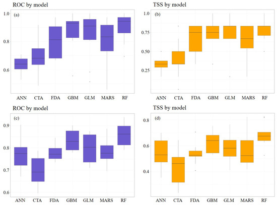
Figure 3.
Accuracy of the single-species distribution model by (a,b) using the trees exhibiting collective dieback and (c,d) using the individual trees exhibiting dieback.
Therefore, we selected these three models for our study. Based on these selected models, an ensemble model was implemented by assigning weights to individual SDMs that showed a true skill statistic (TSS) value of 0.7 or higher [31]. These tasks were performed using the R packages Biomod2 and ggplot2 [32,33].
The results of the model are presented as probabilities, which may result in subjective interpretations [34]. In this study, the threshold was set at the point where the sum of the model’s sensitivity and specificity peaked, and it was used to convert the output of the model [35].
The model was validated using the area under the receiver operating characteristic curve (AUC) and TSS values. The AUC value ranges from 0.5 to 1.0, with a value closer to 1.0 indicating better model performance, and a value of 0.8 or above being considered excellent [36]. The TSS value ranges between −1 and +1, with values closer to +1 indicating better performance [31].
3. Results
3.1. Comparison of Characteristics between Areas of Pinus densiflora with Dieback and Growth
The results showed that all continuous variables (elevation, TWI, age class, and slope degree) exhibited statistically significant differences between the two forest areas (Table 3), whereas all categorical variables (aspect direction, wind exposure, and topographic position), except rock exposure, showed statistically significant associations (Table 4).
Table 3.
Differences in environmental variables between regions based on the Mann–Whitney U test.
Table 4.
Relevance of environmental variables in regions based on chi-squared test.
Among the areas in which pine trees exhibited dieback, the proportion of ridge areas was relatively high (91.4%), TWI was low (2.7), and areas with wind exposure classified as “exposed” accounted for 71.4% of the total. Furthermore, in comparison with the growing areas, the dieback rates were higher in the high-elevation west and southwest slope directions, with rates of 25.7 and 22.9%, respectively.
Under the same conditions, the proportion of ridge areas in the growing region was 41.1%, while 45.5% of the areas with wind exposure were classified as “exposed.” Furthermore, the TWI was higher (3.3) in the growing areas than in the dieback areas, and the aspect direction rate was 18.6% in the west slope direction and 19.4% in the southwest slope direction.
The growing areas showed a tendency for steeper slopes compared to the dieback areas, likely because the average slope in the conservation areas was relatively steep at 32.2°. Because most of the dieback areas were located on ridge terrain, they were considered to have lower values compared to the average slope.
Overall, considering the environmental conditions of the areas with dieback of pine trees within the conservation area, it was found that the dieback was prominent in dry locations with low TWI in ridge areas that were highly exposed to wind. In particular, the proportion of dieback was high (88.6%) in more than six age classes and was concentrated in the southeast-southwest-west direction, accounting for 67.6% of the total population (Figure 4 and Figure 5).
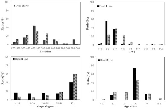
Figure 4.
Comparison of characteristics between dieback and growing areas using continuous variables.
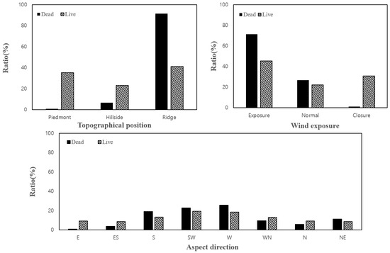
Figure 5.
Comparison of characteristics between dieback and growing areas using categorical variables.
3.2. Evaluation of Areas at Risk for Pine Tree Dieback and Model Evaluation
We established three individual models using the collective dieback area points and repeated the process 10 times, resulting in 30 individual SDMs. The mean AUC value was the lowest for the GLM model (0.892), whereas the mean TSS value was relatively low at 0.75 for the GBM model. The RF model based on machine learning produced the highest AUC and TSS values, and most of the models exhibited excellent performance (Figure 6). An ensemble model was implemented by assigning weights to 20 individual SDMs with TSS values of 0.7 or higher. Both the AUC and TSS values were close to 1.0, and the cutoff threshold value was 520. For model evaluation, we used the permutation importance method to calculate the variable importance [37]. The most important variable was age class, with a contribution of 31%, followed by topographical position (13%), TWI (11%), and aspect direction (8%). Wind exposure, which was recorded as an important variable in previous research, had a relatively low contribution of 2%.
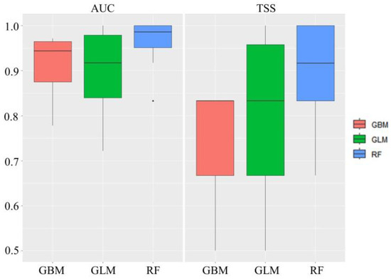
Figure 6.
Evaluation of single models used on the trees exhibiting collective dieback. AUC: area under the receiver operating characteristic curve; TSS: true skill statistic; GBM: generalized boosted model; GLM: generalized linear model; RF: random forest.
We conducted an analysis using individual dieback points using the same method as that used previously, and compared the average AUC and TSS values to those obtained from collective dieback area points, resulting in a decrease in all models. The average AUC and TSS values from the GLM were relatively low at 0.776 and 0.579, respectively, whereas the remaining two individual models showed TSS values of 0.6 or higher and AUC values of 0.8 or higher (Figure 7). An ensemble model was implemented by assigning weights to 10 individual SDMs with TSS values of 0.7 or higher. The AUC and TSS values were 0.988 and 0.894, and the cutoff threshold value was 579. When evaluating the models, the most influential variable was the topographical position, accounting for 27% of the contribution, followed by aspect direction (15%), TWI (11%), and elevation (6%), whereas wind exposure accounted for 2%. The ensemble results using collective dieback area points and individual dieback points are shown in Figure 8.
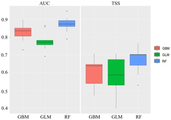
Figure 7.
Evaluation of single models used on the individual trees suffering dieback. AUC: area under the receiver operating characteristic curve; TSS: true skill statistic; GBM: generalized boosted model; GLM: generalized linear model; RF: random forest.
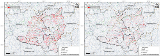
Figure 8.
Maps predicting the area at risk of pine tree dieback using (a) trees collectively suffering dieback and (b) individual trees suffering dieback.
3.3. Evaluation of Areas at Risk of Pine Tree Dieback Using Ensemble Models
To evaluate the areas at risk of pine tree dieback within the conservation area, we used an ensemble method with collective dieback area points and individual dieback points, and presented the priorities in a step-by-step manner to facilitate their application in the field. If both results classified a location as a dieback area, we categorized it as a “caution” area, and if dieback was classified in only one of the two results, the location was categorized as an “interest” area (Figure 9). Based on this spatial distribution, the dieback caution area was 365 ha, whereas the dieback interest area was 572 ha.
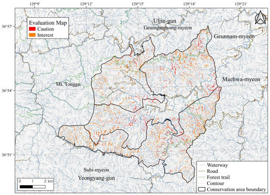
Figure 9.
Predicted map for area at risk of pine tree dieback based on the two results of the ensemble model.
4. Discussion
In this study, samples were extracted from pine tree dieback and growth areas using remote sensing and field surveys. Using this approach, the topographical and environmental characteristics of pine tree dieback were identified, and areas of future risk of pine tree dieback were predicted using an ensemble model that combines three models (GLM, RF, and GBM). The results showed that all three models were highly accurate based on the collective dieback samples, but had a relatively low accuracy based on individual tree dieback samples. It was estimated that this was due to the various topographical and environmental characteristics of the individual tree diebacks. Through this approach, it was confirmed that performing an analysis based on collective dieback sample information was more efficient, and that the RF and GBM models used in the analysis showed excellent performance regardless of the number of samples. Therefore, if similar studies are conducted, the RF and GBM models can be considered primary options, and a comparison for developing SDMs can help select the optimal model.
The main topographical and environmental characteristics of the pine dieback area were high exposure to wind and low TWI compared to the levels in the growth area. In particular, the dieback rate was high among trees of age class 6 or older, and dieback was concentrated in the southeast-southwest-west aspect, accounting for 67.6% of the total distribution. These results show that pine dieback occurs in areas with high potential for desiccation stress caused by climate change. These results are similar to those of studies by Kim et al. (2017) [15] and Kim et al. (2020) [29] on pine trees in the Sokwang-ri Forest Genetic Resources Reserve.
Based on the distribution of pine tree dieback revealed in this study and in previous research, it can be inferred that pine trees located in areas of unfavorable moisture conditions are more sensitive to drought stress. Generally, the vegetation structure of pine tree communities on barren ridges maintains an edaphic climax, which confers a competitive advantage over other species [38]. While such an environment is advantageous for maintaining pine tree communities, high tree density in dry site conditions can cause difficulties for healthy growth owing to competition for water intake when a continuous water supply is not available. In reality, the regulation of plant density is considered to have a significant impact on water uptake by species, plant structure, and roots, and is a crucial factor for maintaining soil moisture [39,40,41,42]. Considering these points, the regulation of stand density through forest management has a direct and positive effect on soil moisture content and can be considered a useful measure for maintaining the structure of the pine forest community [39]. Further research is essential to determine whether the regulation of stand density through forest management can contribute to the establishment of a management system that can cope with climate change.
Therefore, for the conservation of pine forests, it is necessary to select the areas that require “caution” in terms of dieback risk as priority investigation areas and record detailed information on the target areas through continuous monitoring. However, in some regions, healthy growth of pine trees has been observed despite having similar conditions to dieback pine tree areas. Looking back at these cases, additional research is needed to identify the exact cause of pine tree deaths. Therefore, we propose the following additional investigations. (1) If an analysis of the degree of decay of dieback trees within a collective dieback area is performed and the timing of dieback is estimated using tree ring analysis, it would be possible to evaluate the factors that significantly affect annual tree ring growth. (2) For monitoring, if soil environment or soil microbial research is conducted simultaneously in both dieback and growth areas, a comparative analysis between the two areas would be possible, and a comprehensive analysis of changes in soil according to changes in the vegetation structure in the target area could be conducted. It is expected that such additional research will enable more precise prediction of areas at risk of pine tree dieback in the future.
5. Conclusions
This study aimed to identify the differences in the topographical and environmental characteristics between areas of pine forests suffering from dieback and those exhibiting growth. It also focused on evaluating the areas in the pine forest that are at risk of dieback in the Wangpicheon ELCA. The results showed that most pine tree dieback occurred in their main growth areas, and geographical location, TWI, elevation, and aspect direction were identified as important factors for the evaluation of the model.
This led us to derive a priority investigation area that can provide useful information for selecting target sites for monitoring. This study can serve as a reference to compare dieback characteristics in different regions. However, continuous monitoring is necessary to accurately identify the underlying causes and understand the complex biological interactions within an ecosystem, which can lead to the effective management of pine forests.
Author Contributions
Conceptualization, S.-J.L. and S.-H.O.; software, S.-J.L.; formal analysis, S.-J.L.; investigation, S.-J.L., S.-H.O., D.-B.S. and A.-R.L.; writing—original draft, S.-J.L.; writing—review and editing, S.-H.O.; data curation, S.-H.O.; visualization, S.-J.L. All authors have read and agreed to the published version of the manuscript.
Funding
This research received no external funding.
Data Availability Statement
Not applicable.
Acknowledgments
This study was carried out with the support Daegu Regional Environmental Office and ‘R&D Program for Forest Science Technology (Project No. FTIS 2019149C10-2323-0301)’ provided by Korea Forest Service(Korea Forestry Promotion Institute).
Conflicts of Interest
The authors declare no conflict of interest.
References
- Critchfield, W.B.; Little, E.L. Geographic Distribution of the Pines of the World; US Department of Agriculture, Forest Service: Washington, DC, USA, 1966; pp. 1–97.
- Lee, C.S.; Chun, Y.M.; Lee, H.; Pi, J.H.; Lim, C.H. Establishment, Regeneration, and Succession of Korean Red Pine (Pinus densiflora S. et Z.) Forest in Korea. In Conifers; Gonçalves, A.C., Ed.; InTechOpen: London, UK, 2018; pp. 48–77. [Google Scholar] [CrossRef]
- Iwaizumi, M.G.; Tsuda, Y.; Ohtani, M.; Tsumura, Y.; Takahashi, M. Recent distribution changes affect geographic clines in genetic diversity and structure of Pinus densiflora natural populations in Japan. For. Ecol. Manag. 2013, 4, 407–416. [Google Scholar] [CrossRef]
- IPCC. Climate Change 2021 The Physical Science Basis—Summary for Policymakers; IPCC: Geneva, Switzerland, 2021; pp. 1–32. [Google Scholar]
- Walther, G.-R.; Post, E.; Convey, P.; Menzel, A.; Parmesan, C.; Beebee, T.J.; Fromentin, J.-M.; Hoegh-Guldberg, O.; Bairlein, F. Ecological responses to recent climate change. Nature 2002, 416, 389–395. [Google Scholar] [CrossRef] [PubMed]
- Clark, J.S.; Lewis, M.; Horvath, L. Invasion by extremes: Population spread with variation in dispersal and reproduction. Am. Nat. 2001, 157, 537–554. [Google Scholar] [CrossRef] [PubMed]
- Dawson, T.P.; Jackson, S.T.; House, J.I.; Prentice, I.C.; Mace, G.M. Beyond predictions: Biodiversity conservation in a changing climate. Science 2011, 332, 53–58. [Google Scholar] [CrossRef]
- Jackson, S.T.; Betancourt, J.L.; Booth, R.K.; Gray, S.T. Ecology and the ratchet of events: Climate variability, niche dimensions, and species distributions. Proc. Natl. Acad. Sci. USA 2009, 106, 19685–19692. [Google Scholar] [CrossRef]
- Chen, I.-C.; Hill, J.K.; Ohlemüller, R.; Roy, D.B.; Thomas, C.D. Rapid range shifts of species associated with high levels of climate warming. Science 2011, 333, 1024–1026. [Google Scholar] [CrossRef]
- Villén-Pérez, S.; Heikkinen, J.; Salemaa, M.; Mäkipää, R. Global warming will affect the maximum potential abundance of boreal plant species. Ecography 2020, 43, 801–811. [Google Scholar] [CrossRef]
- Chun, J.H.; Lee, C.B. Assessing the effects of climate change on the geographic distribution of Pinus densiflora in Korea using ecological niche model. Korean J. Agric. For. Meteorol. 2013, 15, 219–233. [Google Scholar] [CrossRef]
- Duan, X.; Li, J.; Wu, S. MaxEnt modeling to estimate the impact of climate factors on distribution of Pinus densiflora. Forests 2022, 13, 402. [Google Scholar] [CrossRef]
- Kim, E.S.; Lee, J.S.; Kim, J.B.; Lim, J.H.; Lee, J.S. Management System for Pinus densiflora, Pine Forests, and Conservation; Korea Forest Research Institute: Seoul, Republic of Korea, 2016; pp. 1–22.
- Kang, S.; Lim, J.H.; Kim, E.S.; Cho, N. Modelling analysis of climate and soil depth effects on pine tree dieback in Korea using BIOME-BGC. Korean J. Agric. For. Meteorol. 2016, 18, 242–252. [Google Scholar] [CrossRef]
- Kim, J.; Kim, E.-S.; Lim, J.-H. Topographic and meteorological characteristics of Pinus densiflora dieback areas in Sogwang-Ri, Uljin. Korean J. Agric. For. Meteorol. 2017, 19, 10–18. [Google Scholar] [CrossRef]
- Elith, J.; Leathwick, J.R. Species distribution models: Ecological explanation and prediction across space and time. Annu. Rev. Ecol. Evol. Syst. 2009, 40, 677–697. [Google Scholar] [CrossRef]
- Nelder, J.A.; Wedderburn, R.W. Generalized linear models. J. R. Stat. Soc. Ser. A 1972, 135, 370–384. [Google Scholar] [CrossRef]
- Breiman, L. Random forests. Mach. Learn. 2001, 45, 5–32. [Google Scholar] [CrossRef]
- Elith, J.; Leathwick, J.R.; Hastie, T. A working guide to boosted regression trees. J. Anim. Ecol. 2008, 77, 802–813. [Google Scholar] [CrossRef]
- Buisson, L.; Thuiller, N.; Casajus, S.; Lek, S.; Grenouillet, G. Uncertainty in ensemble forecasting of species distribution. Glob. Change Biol. 2010, 16, 1145–1157. [Google Scholar] [CrossRef]
- Elith, J.H.; Graham, C.P.; Anderson, R.; Dudík, M.; Ferrier, S.; Guisan, A.; Hijmans, R.J.; Huettmann, F.J.; Leathwick, J.R.; Lehmann, A.; et al. Novel methods improve prediction of species’ distributions from occurrence data. Ecography 2006, 29, 129–151. [Google Scholar] [CrossRef]
- Lim, S.J.; Seo, J.C.; Jang, J.Y.; Kim, J.W.; Park, J.H.; Choi, S.H.; Kwon, Y.J.; Byun, H.G.; Kim, J.B.; Hong, S.B.; et al. Natural Ecology of Wangpicheon Comprehensive Environmental Survey Report; Green Korea United: Seoul, Republic of Korea, 2001; pp. 1–453. [Google Scholar]
- Betts, M.G.; Diamond, A.W.; Forbes, M.A.; Villard, M.-A.; Gunn, J.S. The importance of spatial autocorrelation, extent and resolution in predicting forest bird occurrence. Ecol. Model. 2006, 191, 197–224. [Google Scholar] [CrossRef]
- Segurado, P.; Araujo, M.B.; Kunin, W.E. Consequences of spatial autocorrelation for niche-based models. J. Appl. Ecol. 2006, 43, 433–444. [Google Scholar] [CrossRef]
- Dormann, C.F. Effects of incorporating spatial autocorrelation into the analysis of species distribution data. Glob. Ecol. Biogeogr. 2007, 16, 129–138. [Google Scholar] [CrossRef]
- Pearson, R.G.; Raxworthy, C.J.; Nakamura, M.; Peterson, A.T. Predicting species distributions from small numbers of occurrence records: A test case using cryptic geckos in Madagascar. J. Biogeogr. 2007, 34, 102–117. [Google Scholar] [CrossRef]
- Veloz, S.D. Spatially autocorrelated sampling falsely inflates measures of accuracy for presence-only niche models. J. Biogeogr. 2009, 36, 2290–2299. [Google Scholar] [CrossRef]
- Naimi, B.; Skidmore, A.K.; Groen, T.A.; Hamm, N.A. Spatial autocorrelation in predictors reduces the impact of positional uncertainty in occurrence data on species distribution modelling. J. Biogeogr. 2011, 38, 1497–1509. [Google Scholar] [CrossRef]
- Kim, E.-S.; Lee, B.; Kim, J.; Cho, N.; Lim, J.-H. Risk assessment of pine tree dieback in Sogwang-Ri, Uljin. J. Korean Soc. For. Sci. 2020, 109, 259–270. [Google Scholar] [CrossRef]
- Beven, K.J.; Kirkby, M.J. A physically based, variable contributing area model of basin hydrology/Un modèle à base physique de zone d’appel variable de l’hydrologie du bassin versant. Hydrol. Sci. Bull. 1979, 24, 43–69. [Google Scholar] [CrossRef]
- Allouche, O.; Tsoar, A.; Kadmon, R. Assessing the accuracy of species distribution models: Prevalence, kappa and the true skill statistic (TSS). J. Appl. Ecol. 2006, 43, 1223–1232. [Google Scholar] [CrossRef]
- Thuiller, W.; Georges, D.; Engler, R. Ensemble platform for species distribution modeling. In R Package; Version 2.1.7/r560 BIOMOD2; R Foundation for Statistical Computing: Vienna, Austria, 2013. [Google Scholar]
- Kahle, D.J.; Wickham, H. ggmap: Spatial visualization with ggplot2. R J. 2013, 5, 144–161. [Google Scholar] [CrossRef]
- Sinclair, S.; White, M.; Newell, G.R. How useful are species distribution models for managing biodiversity under future climates? Ecol. Soc. 2010, 15, 8. Available online: https://www.jstor.org/stable/26268111 (accessed on 18 January 2023). [CrossRef]
- Franklin, J.; Wejnert, K.E.; Hathaway, S.A.; Rochester, C.J.; Fisher, R.N. Effect of species rarity on the accuracy of species distribution models for reptiles and amphibians in southern California. Divers. Distrib. 2009, 15, 167–177. [Google Scholar] [CrossRef]
- Franklin, J. Mapping Species Distributions: Spatial Inference and Prediction; Cambridge University Press: Cambridge, UK, 2010; p. 320. [Google Scholar] [CrossRef]
- Thuiller, W.; Lafourcade, B.; Engler, R.; Araújo, M.B. BIOMOD—A platform for ensemble forecasting of species distributions. Ecography 2009, 32, 369–373. [Google Scholar] [CrossRef]
- Woo, D.M. Edaphic Climax Condition and Mechanism in Self-Maintaining Forest. Master’s Thesis, Seoul Women’s University, Seoul, Republic of Korea, 2019. [Google Scholar]
- Wei, X.; Liang, W. Regulation of stand density alters forest structure and soil moisture during afforestation with Robinia pseudoacacia L. and Pinus tabulaeformis Carr. on the Loess Plateau. For. Ecol. Manag. 2021, 491, 119196. [Google Scholar] [CrossRef]
- Bravo-Oviedo, A.; Condés, S.; del Río, M.; Pretzsch, H.; Ducey, M.J. Maximum stand density strongly depends on species-specific wood stability, shade and drought tolerance. For. Int. J. For. Res. 2018, 91, 459–469. [Google Scholar] [CrossRef]
- McDowell, N.; Brooks, J.R.; Fitzgerald, S.A.; Bond, B.J. Carbon isotope discrimination and growth response of old Pinus ponderosa trees to stand density reductions. Plant Cell Environ. 2003, 26, 631–644. [Google Scholar] [CrossRef]
- Zeng, W.; Xiang, W.; Zhou, B.; Ouyang, S.; Zeng, Y.; Chen, L.; Zhao, L.; Valverde-Barrantes, O.J. Effects of tree species richness on fine root production varied with stand density and soil nutrients in subtropical forests. Sci. Total Environ. 2020, 733, 139344. [Google Scholar] [CrossRef]


Disclaimer/Publisher’s Note: The statements, opinions and data contained in all publications are solely those of the individual author(s) and contributor(s) and not of MDPI and/or the editor(s). MDPI and/or the editor(s) disclaim responsibility for any injury to people or property resulting from any ideas, methods, instructions or products referred to in the content. |
© 2023 by the authors. Licensee MDPI, Basel, Switzerland. This article is an open access article distributed under the terms and conditions of the Creative Commons Attribution (CC BY) license (https://creativecommons.org/licenses/by/4.0/).