Influence of the External Environment on the Moisture Spectrum of Norway Spruce (Picea abies (L.) KARST.)

Abstract

The fluctuation of relative humidity and temperature in the surrounding environments of wood products is an important parameter influencing their mechanical properties. The objective of this study was to investigate the complex relationship between the moisture content and mechanical properties of wood as a critical aspect in the design of durable and reliable structures. Over a period of 669 days, a simulated type of experiment was conducted, during which the moisture content and external temperature were continuously measured in a compact profile of Norway spruce (Picea abies (L.) KARST.). The data were processed using quadratic and cubic models to establish a predictive model. It was found that the quadratic models slightly outperformed the cubic models when considering time lags greater than six days. The final model demonstrated a significant improvement in explaining the variance of the dependent variable compared to the basic model. Based on these findings, it can be concluded that understanding the relationship between the moisture content and temperature of wood samples plays an important role in wood’s efficient use, particularly for timber constructions. This understanding is vital for accurately predicting the mechanical characteristics of wood, which, in turn, contributes to the development of more durable and reliable structures.

1. Introduction

Wood, a material utilized for centuries in the construction industry, offers exceptional mechanical properties and suitability for general building applications and outdoor construction. It is a natural, renewable resource known for its availability, ease of processing, and versatility. Being a carbon-neutral material, it stores atmospheric carbon dioxide during its growth phase and retains it even after being processed into building components [1,2,3,4,5,6]. These characteristics make wood an environmentally friendly choice that contributes to carbon sequestration and helps to mitigate the impact of carbon emissions from alternative building materials [3].

Wood’s excellent strength-to-weight ratio allows for efficient load-bearing capacities, while its cellular structure, consisting of lignocellulosic fibers, provides inherent strength and resilience against bending and compression forces [7,8,9,10,11]. Additionally, the unique fiber arrangement of wood enables it to resist lateral loads [12], making it suitable for constructing durable frameworks capable of withstanding various environmental conditions. However, being a hygroscopic material, moisture in wood directly impacts its structural integrity, dimensional stability, and resistance to decay and degradation [13,14,15,16,17,18,19]. An excessive moisture content can lead to undesirable consequences, such as swelling, warping, and loss of strength, compromising the performance and longevity of wood-based products [8,20,21,22]. Conversely, insufficient moisture content can result in shrinkage, cracking, and brittleness, further compromising the material’s mechanical properties [8,10,20,23,24]. Therefore, understanding the intricate relationship between wood’s moisture content and its mechanical behavior is vital for designing durable and reliable wood structures. Due to their different structures, individual wood species may differ in their relationship to the joint actions of moisture and temperature. These structural differences also significantly influence the resulting mechanical properties of the wood [25,26,27].

In the field of timber construction, our study builds upon the findings of two influential research papers. The first paper delved into the primary losses of prestressing force in spruce timber used in transversally prestressed wooden constructions [10]. For 669 days, a simulated experiment was conducted to measure prestressing force, external temperature, and moisture. The findings revealed a significant decrease in prestressing force over time during the primary loss phase, leading to the development of a mathematical model of the losses of prestress force. The paper also highlighted the increasing use of timber in bridge constructions and timber-concrete composites, with specific parameters significantly influencing their long-term behavior. The second paper offered a comprehensive study on the use of transverse prestressing in timber structures, illustrating how environmental conditions can significantly influence the prestressing force and, consequently, the load-bearing capacity and stiffness of these structures [27]. The researchers proposed a mathematical model to predict changes in prestressing force over time based on climatic conditions, underscoring the importance of renewable materials in construction for sustainability.

Building upon these findings, our study utilized the same piece of timber as a sample for measuring temperature and moisture. This decision was based on the strong correlation between temperature and moisture in the aforementioned papers. This investigation was carried out to describe the dependency between the surrounding temperature and the wood moisture of the specimen. Given the complexity of this relationship, special regression techniques were used to handle the multicollinearity inherent in these variables. Specifically, we used principal component analysis and repeated cross-validation methods. By applying these advanced statistical techniques, we aimed to describe the dependency between the surrounding temperature and the wood moisture of the specimen, thereby contributing to the ongoing discourse on the sustainable use of timber in construction [21,27].

2. Materials and Methods

2.1. Materials

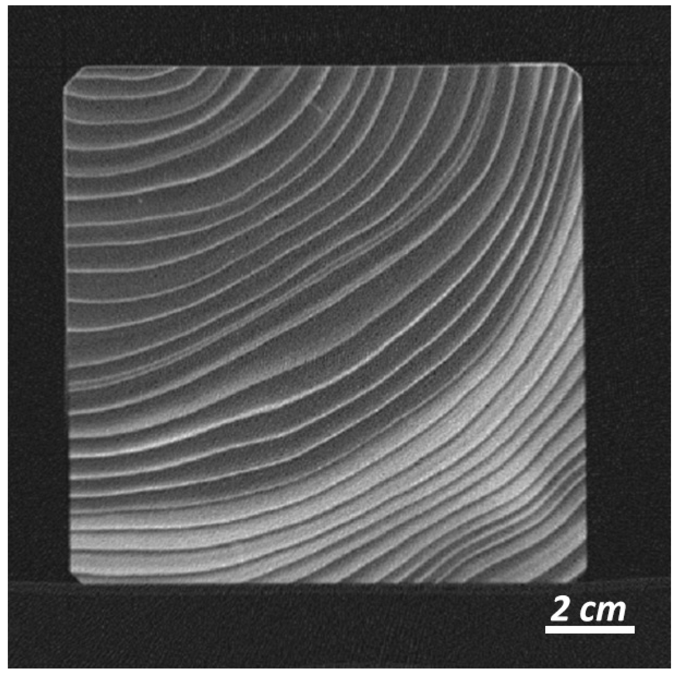
The experiment utilized a compact profile of Norway spruce (Picea abies (L.) KARST.) wood with cross-sectional dimensions of 138 mm × 138 mm and a length of 273 mm, as described in [10,27]. To determine the essential characteristics and ensure the quality of the timber, we measured its average density (oven-dry density) according to the ČSN 49 0108 standard. The recorded density value was 312.0 ± 14.1 kg·m⁻³. Additionally, the density profile was evaluated using an X-ray beam on a QTRS-01X Tree Ring Analyzer (Quintek Measurement Systems Inc., Knoxville, TN, USA). The automated sample measurements, utilizing the QTRS-01X software (Quintek Measurement Systems Knoxville, Knoxville, TN, USA) with a step size of 0.01 mm (Figure 1), provided us with the average growth ring width, measuring 6.48 ± 0.80 mm.

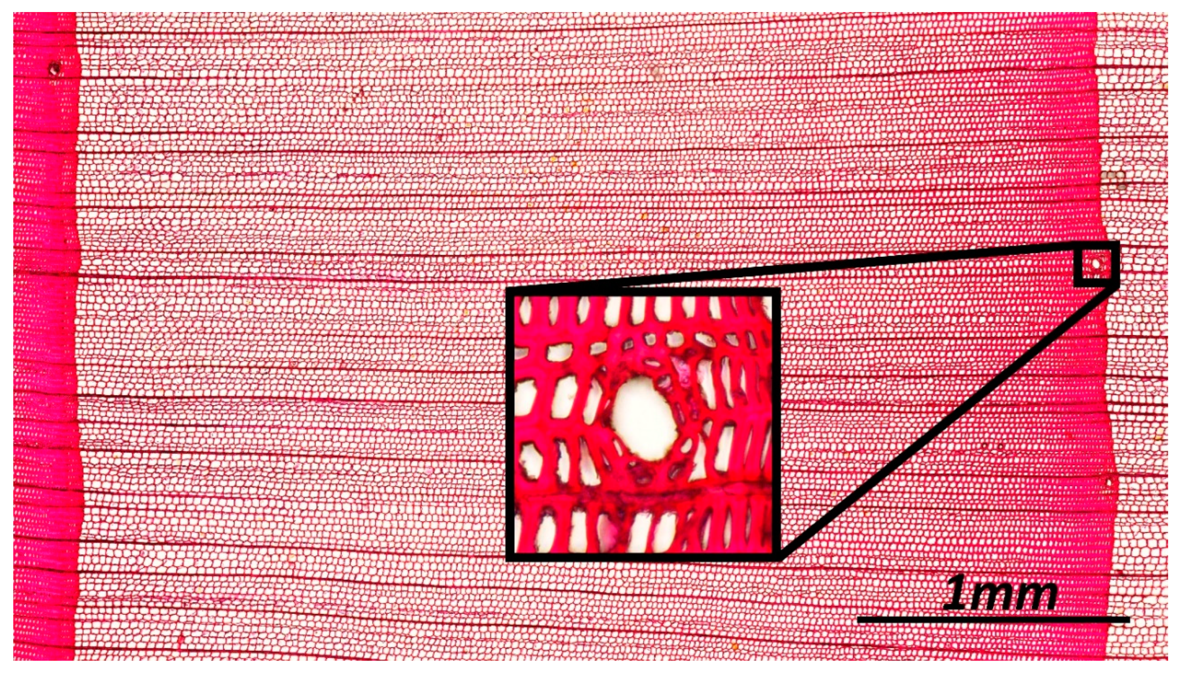
In order to mitigate the potential presence of internal defects such as hidden knots, cracks, or other irregular growth patterns, the sample was subjected to a full-volume CT scan using a Siemens Somatom Scope Power CT scanner (Siemens Healthineers, Erlangen, Germany). Figure 2 represents an illustrative image from this scan, specifically focusing on the area where the temperature and humidity sensors were placed. This comprehensive scan revealed no significant issues that could influence the evaluated properties. Furthermore, a microscopic assessment (Figure 3) was conducted to verify the wood’s classification as spruce.

2.2. Data Collection

The sample was exposed to the exterior environment at VSB TU Ostrava, Faculty of Civil Engineering. Wood moisture content measurements were conducted using the ALMEMO FHA 696 MFS1 sensor (Ahlborn, Holzkirchen, Germany), and temperature values were captured with the ALMEMO FPA 686 sensor (Ahlborn, Holzkirchen, Germany). Data collection was facilitated with the ALMEMO 710 data logger (Ahlborn, Holzkirchen, Germany). The experiment was conducted from 15 November 2016 to 14 September 2018, spanning a total duration of 669 days. The moisture content (M %) and external temperature (T °C) were continuously measured and recorded at minute intervals during this period.

2.3. Initial Observation

The most common indicator for measuring the linear relationship between two variables is the correlation coefficient, which is the reason why it is given first here. Similarly, (ordinary) least squares regression is the simplest and easiest way to model such a relationship. Thus, both can be taken as a good starting point.

The graph in Figure 4 shows the daily averages of the temperature and moisture measurements over the entire experiment, i.e., 669 days from 15 November 2016 to 14 September 2018. One can observe a decrease in the moisture content during the days with temperatures above 15 °C and an increase when the temperatures were low. This expected behavior fully agrees with the calculated value of the correlation coefficient, which is $cor\left(T,M\right)=-0.7022$.

Figure 4. Daily means of measured temperature (red points/values/axis) and moisture (blue points/values/axis) values during entire experiment. (Ordinary) least squares regression leads to the following linear function:

Figure 4. Daily means of measured temperature (red points/values/axis) and moisture (blue points/values/axis) values during entire experiment. (Ordinary) least squares regression leads to the following linear function:

$$M=18.12-0.09013T,$$

(1)

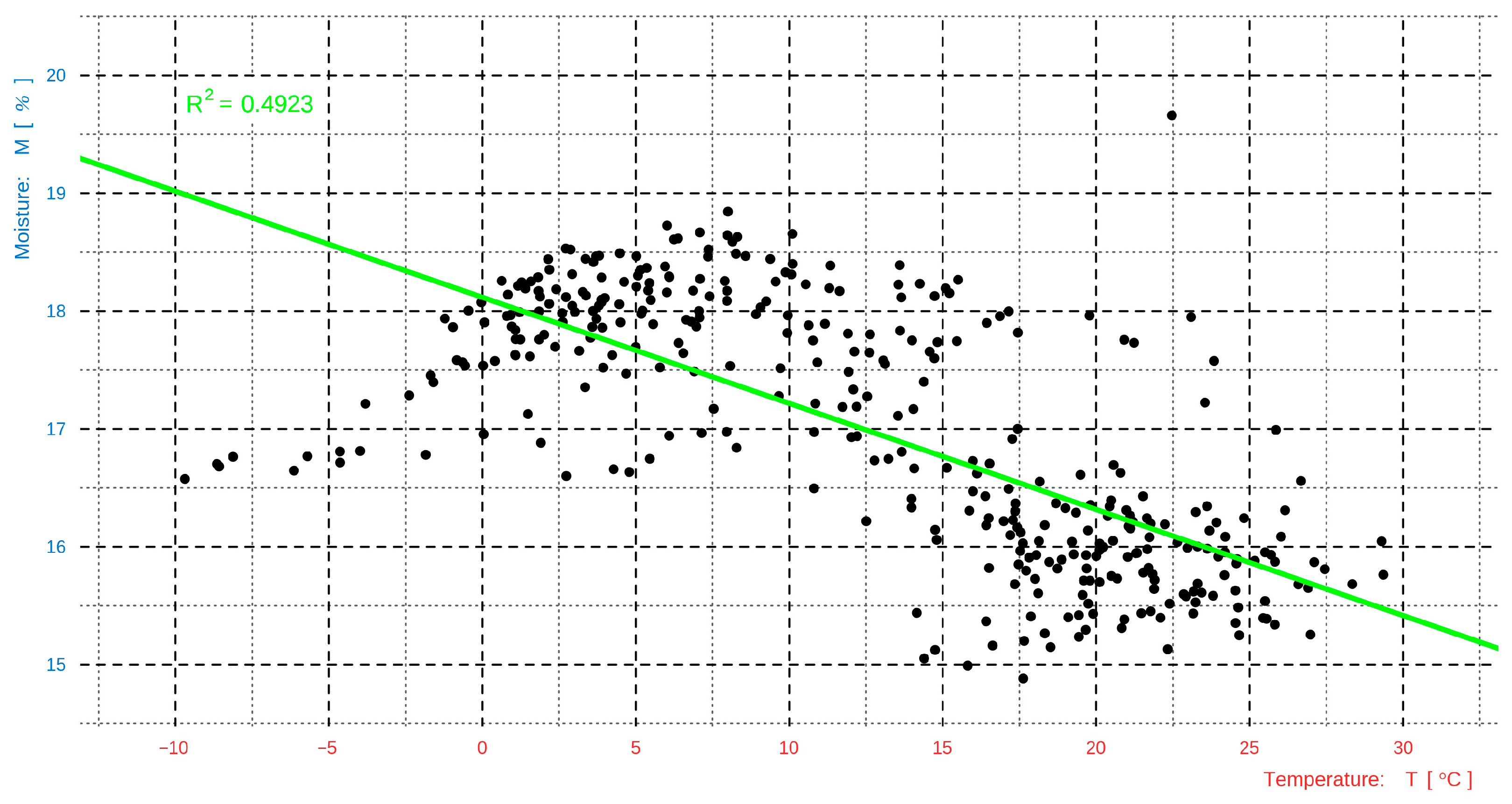
where the negative coefficient of −0.09013 once again indicates decreasing moisture values with increasing temperature. The formula results, compared with the measured values, are shown in the scatter plot in Figure 5. Each point on the plot has coordinates given by the measured temperature and moisture values. The predicted values are represented by the green line. The closer the points on the scatter plot are to the predicted curve, the better the model fits. Here, one group of points above the line (temperatures around 5 °C and moisture around 18%) and another group below the line (temperatures around 20 °C and moisture around 16%) can be seen.

Several indicators can be used to describe the quality of the model and its performance. Among them, R-squared, R²; the root mean square error, RMSE; the mean absolute error, MAE; the Nash–Sutcliffe efficiency coefficient, NSE; and the performance index, PI, are used here. While R², the RMSE, and the MAE are widely and regularly used, efficiency indices and other information criteria are not as common. However, with advances in the use of machine learning methods, these indices are gaining increasing use. In [28], the model and its features were selected based on the RMSE and Wilmott’s efficiency coefficient d, with Wilmott’s d being the basis of the performance index, PI, used here.

The Nash–Sutcliffe efficiency index is defined in [29], and a recent comparison with other indices can be found in [30]. Its power as a model performance criterion was successfully demonstrated in [31,32].

The R-squared, R² (or so-called coefficient of determination), can be viewed as the percentage of variance of the dependent variable explained by the model. Its values range is [0, 1], with a value of 1 indicating a perfect fit; obviously, the higher the value is, the better the model is.

Both the root mean square error, RMSE, and the mean absolute error, MAE, are measures of the error between the observations and the predicted values. Both are non-negative, with 0 being a perfect fit; of course, the lower the value is, the better the model is. The RMSE and MAE values are expressed in the same unit terms as the observations, so that they are easy to interpret.

Finally, two quantifiers of model quality are used, namely, the Nash–Sutcliffe coefficient of efficiency, NSE, and the performance index, PI. Both characterize the predictive power of the model, the difference being their sensitivity to outliers of the predictors and, hence, the predictions.

The NSE values range is $(-\infty ,1]$, with negative values indicating an unsuitable model; NSE = 0 for the predictive power of the average observation and $NSE=1$ indicates a complete fit. Usually, a model with $NSE>0.6$ is considered good.

The value of the efficiency index, PI, is calculated as the product of the Willmott (efficiency) index d and the Pearson correlation coefficient r. The value of PI ranges from 0 to 1. This index, PI, together with the following evaluation table, was proposed by Camargo in [33]. More information about related topics could be found in [34], where a wide range of model performance indices are discussed. Based on PI, the model is considered poor for $PI\le 0.6$, satisfactory for $0.6<PI\le 0.65$, good for $0.65<PI\le 0.7$, and, finally, very good for $PI>0.7$.

The values describing the linear model are:

$$R^2=0.4923,\hspace{1em}\hspace{1em}RMSE=0.8499,\hspace{1em}\hspace{1em}MAE=0.6309,\hspace{1em}\hspace{1em}NSE=0.493,\hspace{1em}\hspace{1em}PI=0.5655.$$

These values are not very satisfactory, and therefore, the model needs to be improved.

Note that the values of R² and NSE are very close to each other, which is a common property of these measures. Their main difference lies in usage; while R² quantifies the goodness of fit of a given statistical model, NSE indicates how well the outcome is predicted by the model simulation. The R² is computed on the same dataset on which the model is trained, while the NSE can be used on completely new, unknown data. This is the reason why the NSE is preferred when evaluating model performance. Therefore, the NSE, rather than R², will be examined in all the considerations below.

2.4. Data Processing

2.4.1. Reasons for the Insufficiency of the Linear Model

The quality of the linear model may be affected by the length of the experiment. Here, its duration was less than two years. This yielded a disbalance between the observations from different seasons. Specifically, in the Central European climate conditions, the experiment took place in Ostrava, which meant a shortage of autumn measurements.

Thus, in order to deal with this problem, we decided to use values measured across one whole year. The second and more likely reason is the insufficiency of temperature as a predictor. This is because the effect of temperature is not instantaneous, i.e., a time lag must be assumed, and therefore, the moisture models, as a function of previous temperatures, must be verified.

There are (at least) two ways to incorporate previous temperatures into the model. The first is to use the past values themselves; the second is to use the past values in terms of their moving averages.

Polynomial, i.e., quadratic, cubic, and biquadratic models should also be investigated, since the moisture and temperature correspondence need not to be linear.

2.4.2. Year Choice

There are several options for choosing the year in which the model will be trained. Although the first and, in a sense, most natural option was to use 2017, the year starting 1 July 2017 and ending 30 June 2018 was chosen.

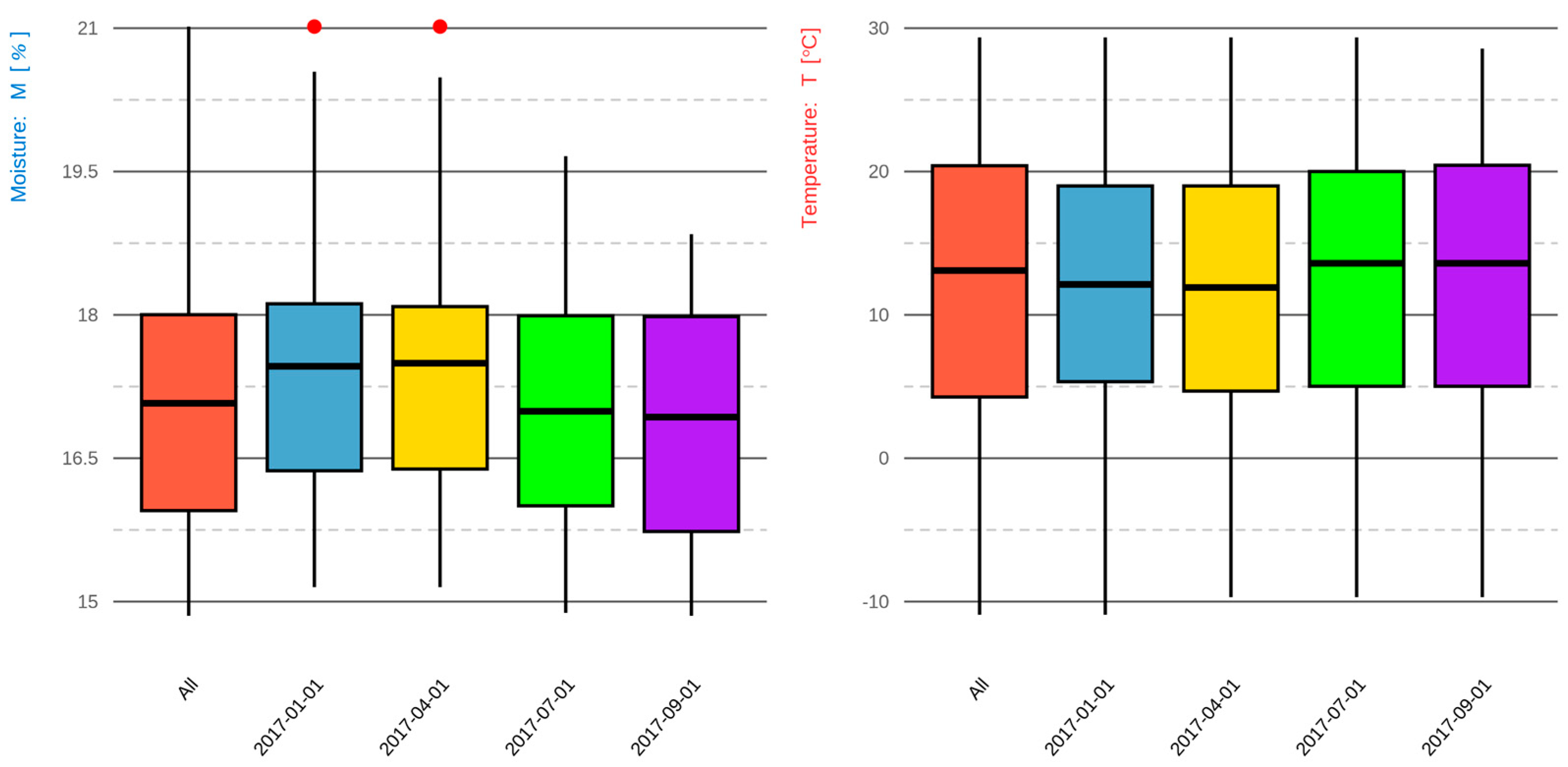
The reasons for this decision are illustrated by the box plots in Figure 6 and the associated

Table 1. Moisture measurement characteristics.

	All	1 January 2017	1 April 2017	1 July 2017	1 September 2017
Min	14.227	15.151	15.151	14.882	14.851
1st Q	15.947	16.369	16.387	16.002	15.733
Median	17.069	17.462	17.494	16.992	16.931
Mean	17.008	17.326	17.287	17.003	16.864
3rd Q	18.001	18.116	18.087	17.991	17.982
Max	21.017	21.017	21.017	19.66	18.845
IQR	2.054	1.747	1.699	1.989	2.249
sd	1.195	1.073	1.025	1.07	1.183

and

Table 2. Temperature measurement characteristics.

	All	1 July 2017	1 April 2017	1 July 2017	1 September 2017
Min	−12.746	−12.746	−9.692	−9.692	−9.692
1st Q	4.271	5.306	4.685	5.019	5.019
Median	13.068	12.121	11.91	13.599	13.599
Mean	12.302	11.781	11.745	12.561	12.773
3rd Q	20.392	18.994	18.994	20.003	20.437
Max	29.357	29.357	29.357	29.357	28.577
IQR	16.121	13.688	14.309	14.984	15.419
sd	9.307	8.619	8.42	8.722	8.958

. Through them, five different time periods are compared, specifically, the entire experimental period and the years starting with the given dates, i.e., 1 January 2017, 1 April 2017, 1 July 2017, and 1 September 2017.

The goal is to find a year that most closely matches the measurement for the entire period. The moisture boxplot, as seen in Figure 6, shows that there are outliers in the cases 1 July 2017 and 1 April 2017 and also that the median moisture values in these years are higher than the median for the whole experiment. The years 1 July 2017 and 1 September 2017 look similar to the whole period. This assessment is supported by the values in Table 1, where the exact differences in the medians and other statistical characteristics can be observed. The final selection of 1 July 2017 was due to its IQR (interquartile range) value, which is close to the moisture IQR for all the data. This choice was tested with the Kruskal–Wallis (rank sum test) and Dunn (multiple comparison) post hoc tests, which confirmed this decision.

The temperature measurements were examined and tested in a similar manner, and no differences were found between the proposed years. Therefore, the moisture-based selection described above remains valid.

Thus, all the models were trained on the dataset derived from the observations from the year between the dates of 1 July 2017 and 31 August 2018. Surely, the rest of the measurements were not discarded but were used further as model testing data.

2.4.3. Predictor Choice

As mentioned above, one way to improve the power of the model is to add more predictors and increase the degree of the formula, i.e., to also examine quadratic, cubic, etc., polynomial regression.

As an equally important option, one should examine the effect of past temperatures, i.e., describe the current moisture value in terms of lagged temperatures, T_i, where the index i denotes the number of days lagged. For example, T₁ is yesterday’s temperature.

Moving averages can also be used. Let ma(T)_i,j denote the moving average of the temperature over i days with a lag of j days. Here, for example, ma(T)_3,0 is the three-day moving average with the current day temperature included. Similarly, ma(T)_5,1 is a five-day moving average starting with yesterday’s temperature.

The plots in Figure 7 indicate the impact of the dependence between humidity and lagged temperature in the correlation coefficients, their powers, or moving averages on the lag length.

It can easily be observed that adding an increasing number of lag days does not necessarily lead to an increase in the correlation. The highest value for the linear term of temperature is reached with a lag of 7 days, and it is equal to $cor(M,T_7)=-0.738$, while for the quadratic term, a lag of 3 days is the best choice, with the value $cor(M,T_3^2)$ $=-0.7721$.

The same is true for increasing the degrees of the polynomial terms, where the lowest correlation coefficient is obtained for the highest power considered, i.e., for the biquadratic terms of $T_i^4$. The highest correlation appears in the case of the quadratic terms $T_i^2$.

The right-hand side of Figure 7 shows the situation for the moving averages, which is different, because the correlation coefficients do not change significantly when time lags are added. In ma_i,j (with T for temperature omitted here), the first index i indicates the number of days for the moving average, while the second index j indicates the length of the time shift, e.g., ma_5,3 is a moving average of 5 days shifted by 3 days.

In all cases, the maximum values are around −0.76 for moving averages of 7 or 8 days. Their differences are of the order of hundredths. This is neither a problem nor an argument for excluding the time-lagged moving averages from further consideration. The reason why time-lagged moving averages are examined is the possibility of their use together with the temperature values of T. Since moving averages are (of course) computed from expressions of T, their joint use causes multicollinearity of the predictors in the regression model.

The above discussion led to the decision to investigate models containing temperature terms with a maximum lag of 7 days and a polynomial of degree 3. The maximum length of the considered moving average was also set to 7 days.

This decision was based not only on the above discussion but also on the natural assumption that temperatures with a time lag of more than 7 days are too distant to affect the actual moisture.

Similar reasoning led to the elimination of the actual temperature terms, since temperature cannot affect moisture instantaneously. Furthermore, a strong relationship between the current (e.g., today’s) temperature T and the previous day’s (e.g., yesterday’s) temperature T₁, expressed by a correlation coefficient equal to $cor(T,T_1)=0.9688$, must be taken into account.

Although the correlation coefficients of these terms suggest a strong relationship, their rejection seems to be meaningful from a physical point of view. The goal is to construct not a mathematical model with the highest rank but a model corresponding to the real conditions.

2.5. Model Preparation

After the above reduction in the number of possible predictors, 21 predictors still remained, specifically, temperatures with a time lag of a maximum of 7 days and their first, second, and third powers.

Building a model with such a large number of predictors is tedious, as well as time- and power-consuming, and more importantly, because the temperature terms are correlated, there is still the possibility that the resulting model will be overestimated.

The following steps can be taken to address this problem. One starts with a simple least squares regression model with all the predictors and checks not only the useful measures, such as the R-squared or RSS, but also, in particular, the significance of the coefficients obtained. Those predictors that do not meet the criteria (p-value and significance level) can be rejected and the model can be rebuilt without them. These steps are repeated until a model with the desired properties is obtained.

The described procedure need not to be performed manually in a loop, since there are special predictor selection methods to speed it up.

Here, the so-called stepAIC method was used. This method builds models based on different subsets of the considered predictors and selects the one with the lowest AIC value, where AIC stands for the Akaike Information Criterion. This criterion quantifies the loss of information caused by modifying the set of predictors. This modification can be performed through a forward step, i.e., adding a new predictor; a backward step, i.e., removing a predictor; or the combination of both directions.

The AIC penalizes the model for adding more variables to it. Its absolute value is not important, because the procedure only compares its tendency, i.e., whether it decreases or increases as the predictors change. This is similar to the modified R-squared used in ordinary least squares methods.

This criterion was introduced by Akaike in [35], and its usage was further developed over time. A comprehensive summary of its use in statistical modeling and a selection of regression models can be found in [36].

The procedure of the model’s preparation and its final tuning and testing was implemented in the statistical computing language R [37] in its IDE (Integrated Development Environment), RStudio [38], with the help of the specialized packages MASS [39] and Caret (Classification and Regression Training) [40] for model preparation, tuning, and final selection and Tidyverse [41] for the initial data description, analysis, tidying, and cleansing. Finally, ggplot2 [42] was used for the visualizations.

Illustration of Modeling Procedure

According to the procedure described above, 30 ordinary least squares models were prepared. These models were divided into three groups: models containing only linear terms (denoted as Linear), models containing linear and quadratic terms (denoted as Quadratic), and finally, models combining linear, quadratic, and cubic terms (denoted as Cubic). There were 10 models in each of these groups, each based on a different number of lagged temperature values.

We denoted these models as $L_{ols}^i$, $Q_{ols}^i$, and $C_{ols}^i$, where L stands for Linear, Q for Quadratic, and C for Cubic; the superscript i denotes the maximum lag length number used here; and the subscript denotes the method used, i.e., ols stands for ordinary least squares here.

In this notation, $Q_{ols}^3$ is a quadratic model with a maximum lag of 3 days, i.e., an ordinary least squares model predicting moisture based on $T_1$, $T_1^2$, $T_2$, $T_2^2$, $T_3$, and $T_3^2$. Together with the intercept, 7 coefficients need to be found.

Increasing the number of lagged temperatures and their powers yields longer and, therefore, more complicated formulas. For $Q_{ols}^3$, considered here, one obtains the following formula:

$$Q_{ols}^3=17.82+0.03486T_1-0.002875T_1^2-0.02456T_2+0.0004491T_2^2+0.01611T_3-0.00249T_3^2.$$

The prediction power of this formula is described with these values:

$$\begin{gathered} \mathit{Training}:RMSE=0.6674,MAE=0.5177,NSE=0.61,PI=0.6776, \\ \mathit{Testing}:RMSE=0.7451,MAE=0.5728,NSE=0.6123,PI=0.6743, \end{gathered}$$

where the first set of model characteristics are computed on the training dataset, i.e., the year from 1 July 2017 to 30 June 2018, and the second set of characteristics are computed on the entire dataset, i.e., the observations from the entire experimental period, which serve here as the test dataset.

The main difference between the training and test evaluations is in the measures of the RMSE and MAE, which are increased using all the data. The values of the performance indicators NSE and PI remain almost the same.

After building, exploring, and rating the ordinary least squares model, the stepAIC procedure is performed to improve the predictive power of the model and reduce the number of predictors used.

The above model $Q_{ols}^3$ is transformed into a new model $Q_{aic}^3$ in the following form with the following prediction power:

$$Q_{aic}^3=17.83+0.253T_1-0.002715T_1^2-0.002159T_3^2.$$

(2)

$$\begin{gathered} \mathit{Training}:RMSE=0.6678,MAE=0.5184,NSE=0.6096,PI=0.6772, \\ \mathit{Testing}:RMSE=0.7446,MAE=0.5729,NSE=0.6129,PI=0.6747. \end{gathered}$$

As can easily be observed, the RMSE, MAE, NSE, and PI values remain the same; thus, the improvement lies in the reduction in the number of predictors. The $Q_{ols}^3$ formula contains 7 terms, namely, the intercept and 6 lagged temperatures, while $Q_{aic}^3$ contains only 4, i.e., the intercept and 3 temperature terms, and only 2 of them are quadratic.

3. Results and Discussion

3.1. Model Comparison and Rating

In order to compare the performances of all the models developed,

Table 3. The performance characteristics of proposed ordinary least square models; (L—linear, Q—quadratic, C—cubic; for different time lags).

		RMSE			MAE			NSE			PI
Lag	L	Q	C	L	Q	C	L	Q	C	L	Q	C
0	0.847	0.786	0.774	0.640	0.601	0.564	0.499	0.568	0.582	0.565	0.632	0.648
1	0.835	0.772	0.765	0.634	0.59	0.558	0.513	0.583	0.591	0.579	0.647	0.657
2	0.823	0.759	0.754	0.625	0.583	0.548	0.527	0.597	0.603	0.592	0.660	0.669
3	0.812	0.745	0.742	0.617	0.573	0.542	0.539	0.613	0.615	0.604	0.675	0.680
4	0.806	0.739	0.737	0.614	0.569	0.541	0.547	0.619	0.621	0.612	0.681	0.685
5	0.803	0.733	0.736	0.611	0.562	0.542	0.550	0.625	0.621	0.615	0.686	0.685
6	0.793	0.728	0.736	0.604	0.559	0.542	0.561	0.630	0.621	0.626	0.691	0.685
7	0.791	0.731	0.736	0.603	0.561	0.542	0.563	0.627	0.621	0.628	0.689	0.685
8	0.790	0.731	0.736	0.603	0.561	0.542	0.565	0.627	0.621	0.629	0.689	0.685
9	0.791	0.731	0.736	0.603	0.561	0.542	0.563	0.627	0.621	0.628	0.689	0.685
10	0.791	0.731	0.739	0.603	0.561	0.545	0.563	0.627	0.619	0.628	0.689	0.683

summarizes their RMSE, MAE, NSE, and PI values calculated on the test data from the whole experimental period. Here, one can find either the one with the lowest error (RMSE or MAE) or the one with the highest predictive ability (NSE or PI).

The use of Table 1 leads to the rejection of all the linear models because none of them satisfy either the NSE or the PI criterion for a good model, namely, NSE < 0.6 and PI < 0.65 for all of them. For the same reason, the quadratic models with a lag of less than 3 days and cubic models with a lag of less than 2 days are also rejected.

In addition, Table 3 also shows the changes in the values of the performance characteristics depending on the change in the type of model, i.e., from quadratic to cubic, or the change in the number of predictors, i.e., the maximum time lag used. These changes are very small, being of the order of thousandths, for time lags longer than 2 days. Therefore, there are again natural questions as to whether the use of multiple predictors will yield the intended goal, i.e., a formula that is not only highly ranked but also easy to use and understand.

The highest values of the NSE and PI are obtained with formula $Q_{aic}^6$, which is given and described as follows:

$$Q_{aic}^6=17.83+0.03612T_1-0.002586T_1^2-0.001022T_2^3-0.002586T_5^2-0.001022T_6^2.$$

(3)

$$\begin{gathered} \mathit{Training}:RMSE=0.6442,MAE=0.4961,NSE=0.6367,PI=0.7019, \\ \mathit{Testing}:RMSE=0.7281,MAE=0.5593,NSE=0.6298,PI=0.6909. \end{gathered}$$

The differences in the RMSE, MAE, NSE, and PI between the best model $Q_{aic}^6$ and the model $Q_{aic}^3$ proposed above are:

$$∆RMSE=-0.01644,∆MAE=-0.01362,∆NSE=0.0169,∆PI=0.01613,$$

Thus, one could conclude that although there is no doubt that $Q_{aic}^6$ outperformed $Q_{aic}^3$ in all the parameters, the level of improvement is not high enough to justify a higher number of predictors.

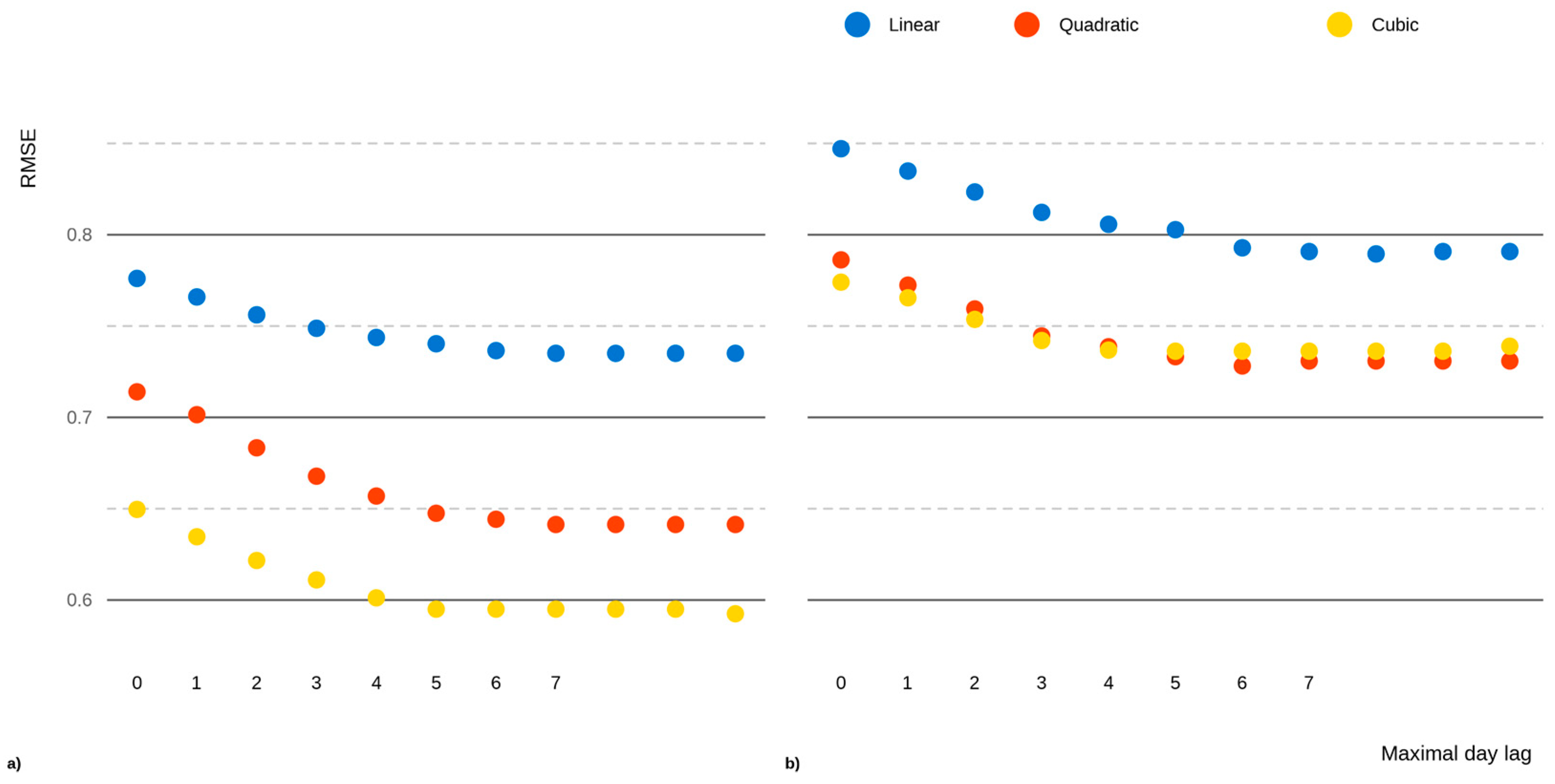
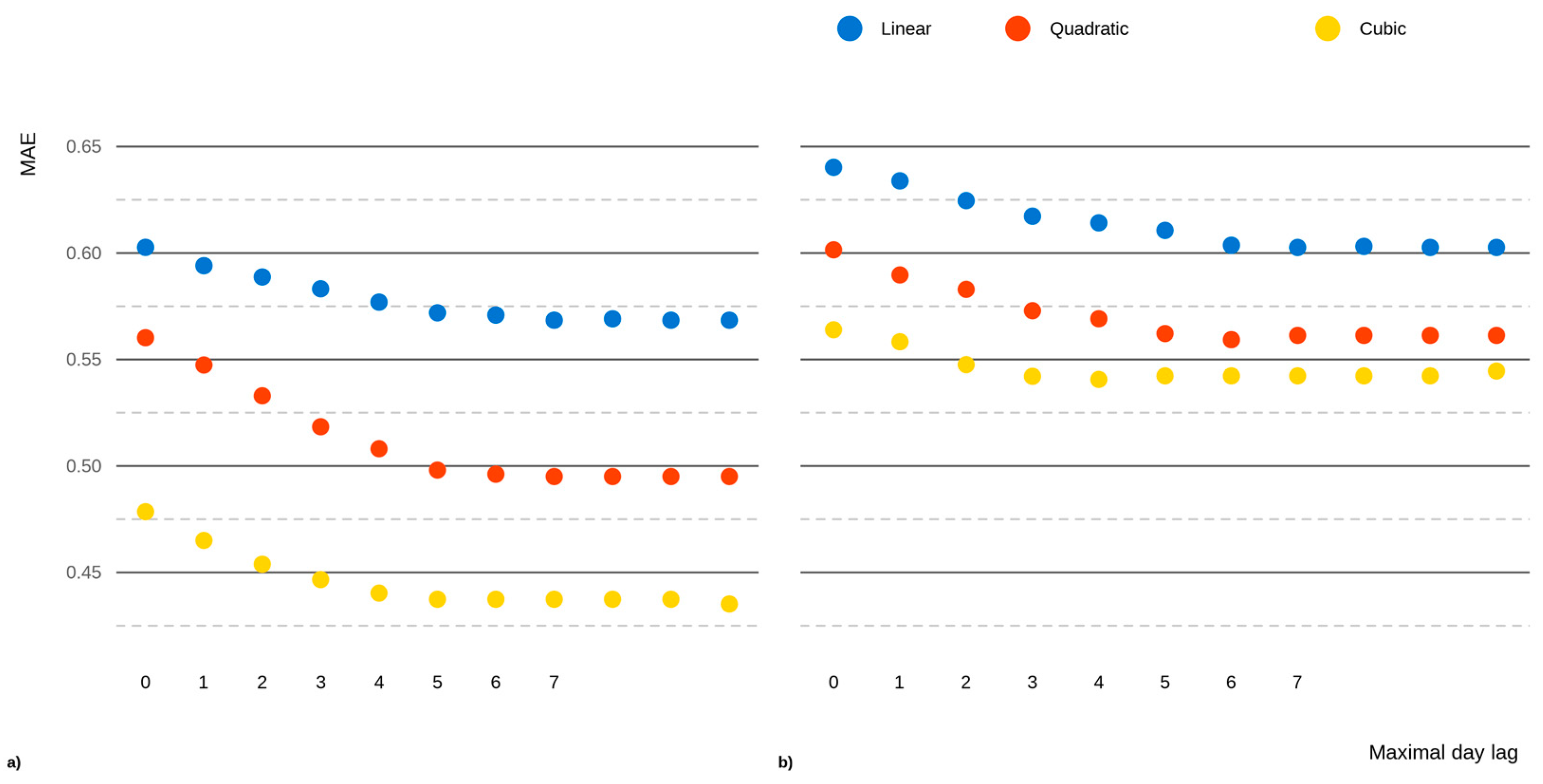
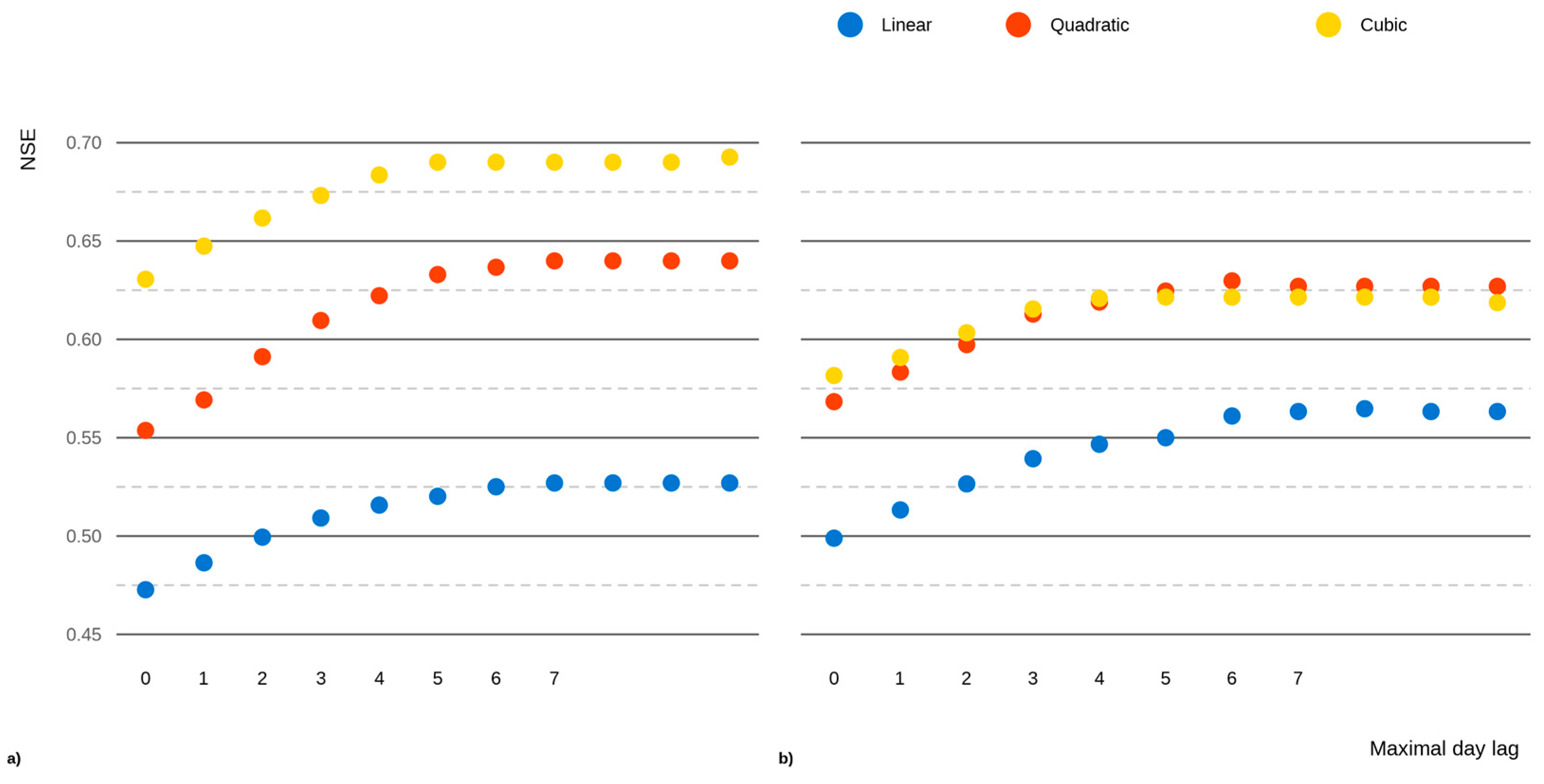
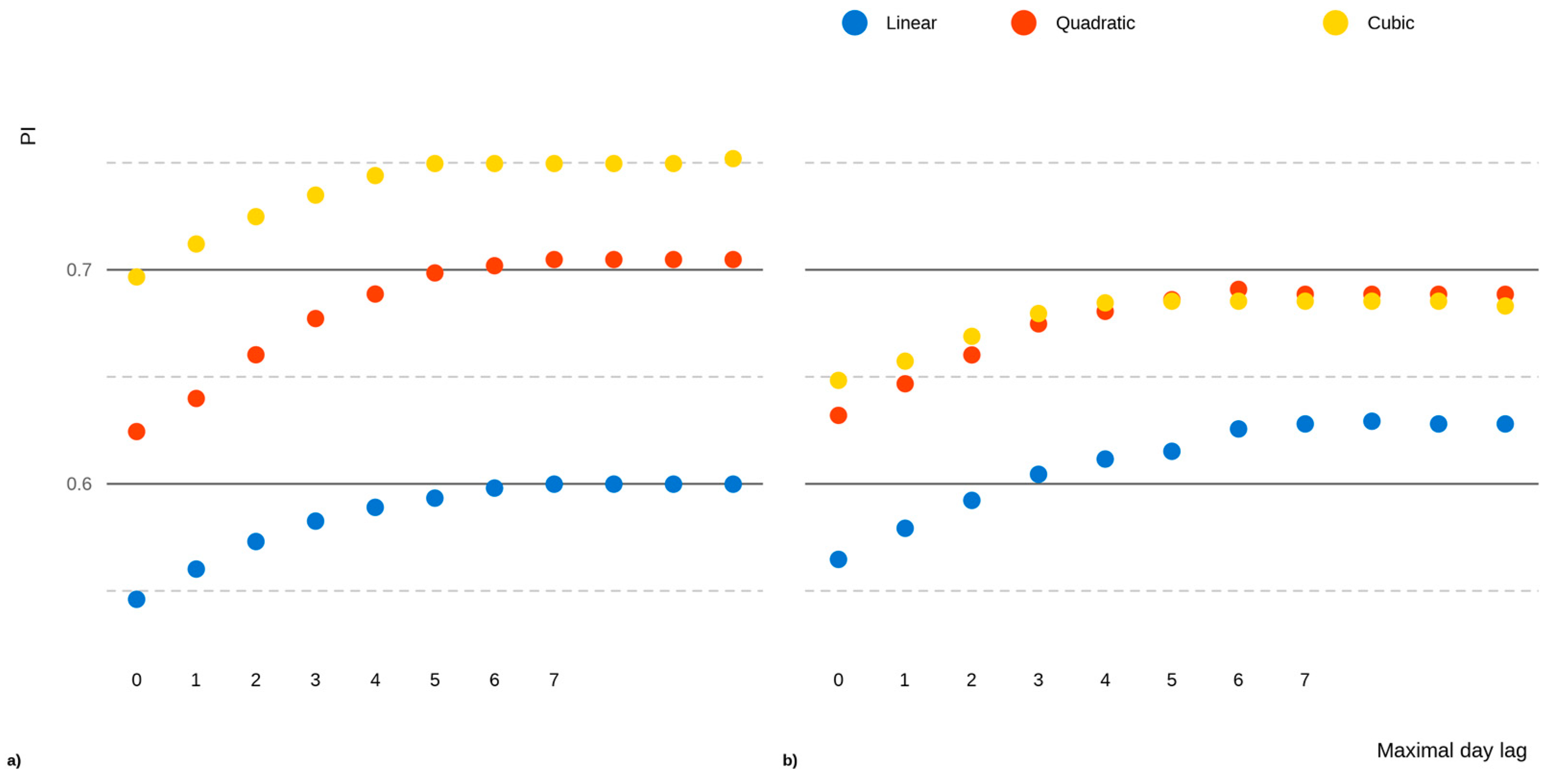
The dependence of the RMSE, MAE, NSE, and PI on the number of predictors, i.e., the time lag used, is also shown in Figure 8, Figure 9, Figure 10 and Figure 11. These figures visually provide the same information as that shown in Table 3. It was possible to observe an improvement in all the characteristics with incrementing time lags until the best value was reached, after which they started to stagnate or even decrease.

The figures show the results for both datasets, i.e., the training and the testing parts. In the training part, the cubic models performed significantly better than the quadratic models. However, the performance examined for testing, i.e., for new and unknown data, is more important in deciding which model to choose. Additionally, at this point, the figures show a noticeable increase in the closeness between the performances of the quadratic and cubic models on the test dataset. Furthermore, note that for the RMSE, NSE, and PI, the quadratic models slightly outperform the cubic models for time lags greater than 6 days.

Finally, note that Table 3 and Figure 8, Figure 9, Figure 10 and Figure 11 confirm the correctness of the assumptions made in the previous sections, particularly the rejection of the models with time lags longer than 7 days. For emphasis, results are also presented for the models with time lags longer than 7 days and up to 10 days.

3.2. Final Tuning

The choice of the quadratic model as the final formula introduces a new problem. The formula $Q_{aic}^3$ is a quadratic function of two variables and as such reaches its global maximum. Specifically, for T₁ = 4.67 °C and T₃ = 0 °C, the maximum moisture predicted by this model is M_max = 17.89%.

The existence of a global maximum is true for all the quadratic and cubic models obtained by means of the method presented above.

In order to solve this problem, the entire model underwent a new tuning process. In this second run, moving averages of different lengths and different time delays were added. Under this new setup, ordinary least squares models were again built and then adjusted using the stepAIC methods.

Then, their RMSE, MAE, NSE, and PI characteristics were calculated and examined, and the models were ranked based on them. Finally, the final model was selected. This was a model derived from the $Q_{aic}^3$ model (2) described in the previous section.

The final model had the form:

$$M=17.91+0.08295T_1-0.004101T_1^2-0.07851{ma\left(T\right)}_{\mathrm{7,1}},$$

(4)

where the ma(T)_7,1 is a moving average of 7 days, shifted by 1 day.

The form of the final model (4) is very simple because the quadratic term $T_3^2$ was suppressed through the stepAIC procedure. The current moisture is therefore given as a linear function of the temperatures of the previous seven days, except for the term representing the previous day, which is quadratic, and such a function cannot be bounded. Thus, the problem of the global maxima and, hence, the bounded predictions is solved.

The predictive power of the final model is given by the following values:

$$\begin{gathered} \mathit{Training}:RMSE=0.6676,MAE=0.5145,NSE=0.6099,PI=0.6775, \\ \mathit{Testing}:RMSE=0.7355,MAE=0.5617,NSE=0.6222,PI=0.6834, \end{gathered}$$

which are slightly better than those of the base model $Q_{aic}^3$, as seen in Equation (2), and slightly worse than those of the model $Q_{aic}^6$, in Equation (3), with the best rank among all the models.

In addition to the above statistics, we computed the coefficient of determination of the final model. This index was mentioned in the Introduction in connection to the basic linear formula in Equation (1). Recall that its value can be understood as a measure of dependent variable variance, which is explained by the model.

The final model (4) reached a value of 0.7016, whereas for the basic model (1), it was only 0.4923. This is a significant improvement, which is also true in the case of all the measures of the final model compared to the basic model.

However, as mentioned above, the model characteristics are not the only criteria that justify the choice of the final model. Its simplicity also needs to be taken into account.

In addition to the numerical characteristics and indices, the performance of the final model is illustrated in two graphs.

The graph in Figure 12 shows the measured and predicted moisture throughout the entire experiment. The significant descriptive values of the measurements and predictions are indicated by the markers on the y-axis; in particular, their minimum, maximum, first and third quartiles, and median are shown.

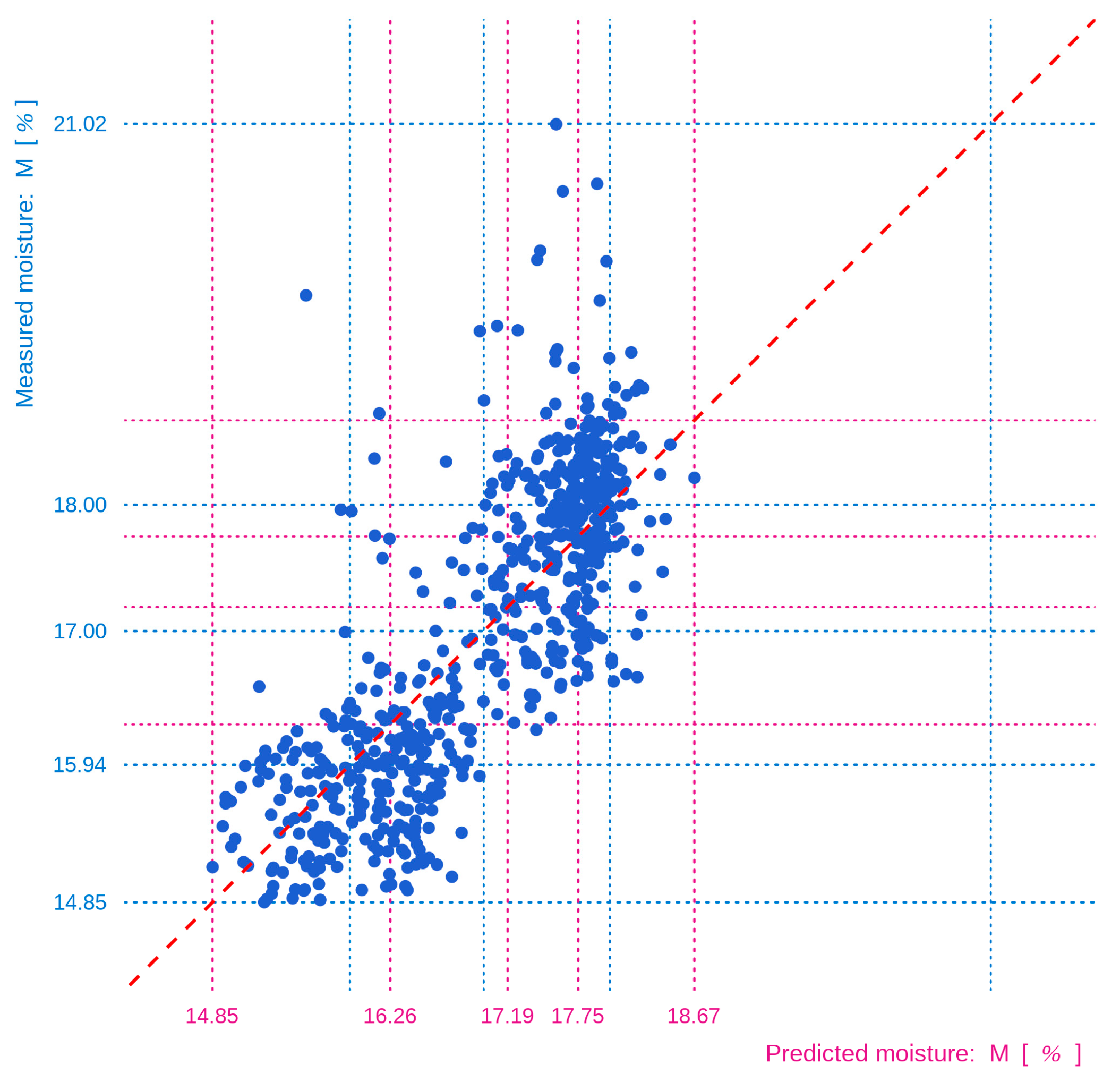
The graph in Figure 13 is a scatter plot that provides a representation of the agreement between the moisture measured and the moisture predicted by the final model. Each point on this graph has coordinates given as a pair (prediction, measurement); the closer the predicted value is to the measured value, the closer it is to the x = y line. The line $x=y$ capturing this ideal state is plotted as a red dashed line in Figure 13. Note that the closer the points are to the x = y line, the higher the NSE value is.

The graph in Figure 12 depicts higher differences between the measurements and simulations for the first half of 2017, and the scatter plot in Figure 13 contains points that are further from the desired x = y line. Thus, it can be seen that the model could not accurately perform predictions in all circumstances. This is due to the fact that it is only a temperature model, which does not take into account other meteorological parameters such as precipitation in the form of either rain or snow in winter.

However, as a simple temperature-based model, the proposed final model is very effective.

4. Conclusions

A simulation experiment was conducted from 2016 to 2018, and the prestressing force, external temperature, and moisture content of wood samples were measured. The main objective of this simulation was to propose a formula describing the dependence of prestress on time, temperature, and the moisture content.

Since temperature and moisture are strongly related, their measurements were re-examined together to obtain a description of their relationship. This was the aim of the work presented in this paper.

Our examination of the data led to the proposal of a model for predicting the actual moisture content as a function of temperature values with different time lags. Decisions regarding the exact length of the time lag and the maximal power of the polynomial temperature term were made based on the results of stepAIC regression methods, which are designed to reduce the number of predictors while preserving (or improving) the predictive power of the regression model. As the proposed model is only a temperature model, it cannot capture all the moisture changes and fluctuations perfectly; to increase its power, other external influences also need to be taken into account. However, based on the evaluation of the final model using multiple statistical indicators, its high predictive ability was proven.

References

1. Buchanan, A.H.; Levine, S.B. Wood-Based Building Materials and Atmospheric Carbon Emissions. Environ. Sci. Policy 1999, 2, 427–437. [Google Scholar] [CrossRef]
2. Karjalainen, T.; Kellomäki, S.; Pussinen, A. Role of Wood-Based Products in Absorbing Atmospheric Carbon. Silva Fennica. 1994. 28, 67–80. [CrossRef] [Green Version]
3. Mantau, U. Wood Flow Analysis: Quantification of Resource Potentials, Cascades and Carbon Effects. Biomass Bioenergy 2015, 79, 28–38. [Google Scholar] [CrossRef]
4. Belgacem, M.N.; Pizzi, A. (Eds.) Lignocellulosic Fibers and Wood Handbook: Renewable Materials for Today’s Environment; Scrivener Publishing: Beverly, MA, USA; Wiley: Beverly, MA, USA; Hoboken, NJ, USA, 2016; ISBN 978-1-118-77352-9. [Google Scholar]
5. Dinwoodie, J.M. Timber; CRC Press: Boca Raton, FL, USA, 2000; ISBN 978-1-135-80810-5. [Google Scholar]
6. Mitterpach, J.; Fojtík, R.; Machovčáková, E.; Kubíncová, L. Life Cycle Assessment of a Road Transverse Prestressed Wooden–Concrete Bridge. Forests 2022, 14, 16. [Google Scholar] [CrossRef]
7. Record, S.J. The Mechanical Properties of Wood: Including a Discussion of the Factors Affecting the Mechanical Properties and Methods of Timber Testing; Publishers Printing Company: New York, NY, USA, 1914. [Google Scholar]
8. Bodig, J.; Jayne, B.A. Mechanics of Wood and Wood Composites; Krieger Pub Co.: Malabar, FL, USA, 1993; ISBN 978-0-89464-777-2. [Google Scholar]
9. Vasiliev, V.V.; Morozov, E.V. Advanced Mechanics of Composite Materials and Structures, 4th ed.; Elsevier: Amsterdam, The Netherlands, 2018; ISBN 978-0-08-102209-2. [Google Scholar]
10. Fojtík, R.; Dubovský, V.; Kozlová, K.; Kubíncová, L. Prestress Losses in Spruce Timber. Wood Res. 2020, 65, 645–652. [Google Scholar] [CrossRef]
11. Wenzel, H. Health Monitoring of Bridges; Wiley: Chichester, UK, 2009; ISBN 978-0-470-03173-5. [Google Scholar]
12. Wadi, H.; Amziane, S.; Taazount, M. The Lateral Load Resistance of Unclassified Cross-Laminated Timber Walls: Experimental Tests and Theoretical Approach. Eng. Struct. 2018, 166, 402–412. [Google Scholar] [CrossRef]
13. Wang, J.; Cao, X.; Liu, H. A Review of the Long-Term Effects of Humidity on the Mechanical Properties of Wood and Wood-Based Products. Eur. J. Wood Prod. 2021, 79, 245–259. [Google Scholar] [CrossRef]
14. Startsev, O.V.; Makhonkov, A.; Erofeev, V.; Gudojnikov, S. Impact of Moisture Content on Dynamic Mechanical Properties and Transition Temperatures of Wood. Wood Mater. Sci. Eng. 2017, 12, 55–62. [Google Scholar] [CrossRef]
15. Vololonirina, O.; Coutand, M.; Perrin, B. Characterization of Hygrothermal Properties of Wood-Based Products—Impact of Moisture Content and Temperature. Constr. Build. Mater. 2014, 63, 223–233. [Google Scholar] [CrossRef] [Green Version]
16. Buell, T.W.; Saadatmanesh, H. Strengthening Timber Bridge Beams Using Carbon Fiber. J. Struct. Eng. 2005, 131, 173–187. [Google Scholar] [CrossRef]
17. Lukowsky, D.; Wade, D. Failure Analysis of Wood and Wood-Based Products; Mc Graw-Hill education: New York, NY, USA, 2015; ISBN 978-0-07-183937-2. [Google Scholar]
18. Obućina, M.; Kitek Kuzman, M.; Sandberg, D. Use of Sustainable Wood Building Materials in Bosnia and Herzegovina, Slovenia and Sweden; University of Sarajevo, Mechanical Engineering Faculty, Department of Wood Technology: Sarajevo, Bosnia and Herzegovina, 2017. [Google Scholar]
19. Fojtík, R.; Dědková, K. Analysis of Diagnostic Methods for Detecting the Presence of Gloeophyllum spp. Wood Res. 2018, 63, 479–486. [Google Scholar]
20. Thybring, E.E.; Fredriksson, M. Wood Modification as a Tool to Understand Moisture in Wood. Forests 2021, 12, 372. [Google Scholar] [CrossRef]
21. Fojtík, R.; Kubíncová, L.; Dubovský, V.; Kozlová, K. Moisture at Contacts of Timber-Concrete Element. Wood Res. 2020, 65, 917–924. [Google Scholar] [CrossRef]
22. Sandberg, K.; Pousette, A.; Nilsson, L. Moisture Conditions in Coated Glulam Beams and Columns during Weathering. In Proceedings of the International Conference on Durability of Building Materials and Components, Porto, Portugal, 12–15 April 2011; pp. 1–8. [Google Scholar]
23. Almeida, G.; Hernández, R.E. Changes in Physical Properties of Tropical and Temperate Hardwoods below and above the Fiber Saturation Point. Wood Sci. Technol. 2006, 40, 599–613. [Google Scholar] [CrossRef]
24. Brischke, C.; Rapp, A.O.; Bayerbach, R. Measurement System for Long-Term Recording of Wood Moisture Content with Internal Conductively Glued Electrodes. Build. Environ. 2008, 43, 1566–1574. [Google Scholar] [CrossRef]
25. Reiterer, A.; Sinn, G.; Stanzl-Tschegg, S.E. Fracture Characteristics of Different Wood Species under Mode I Loading Perpendicular to the Grain. Mater. Sci. Eng. A 2002, 332, 29–36. [Google Scholar] [CrossRef]
26. Zhang, S.Y. Effect of Growth Rate on Wood Specific Gravity and Selected Mechanical Properties in Individual Species from Distinct Wood Categories. Wood Sci. Technol. 1995, 29, 451–465. [Google Scholar] [CrossRef]
27. Fojtík, R.; Dubovský, V.; Kubíncová, L.; Stejskalová, K.; Machovčáková, E.; Lesňák, M. Probabilistic Expression of the Function of the Change in Prestressing Force of Timber Elements Depending on Climatic Conditions in Situ. Constr. Build. Mater. 2023, 377, 130955. [Google Scholar] [CrossRef]
28. Fransson, E.; Eriksson, F.; Erhart, P. Efficient Construction of Linear Models in Materials Modeling and Applications to Force Constant Expansions. NPJ Comput. Mater. 2020, 6, 135. [Google Scholar] [CrossRef]
29. Nash, J.E.; Sutcliffe, J.V. River Flow Forecasting through Conceptual Models Part I—A Discussion of Principles. J. Hydrol. 1970, 10, 282–290. [Google Scholar] [CrossRef]
30. Duc, L.; Sawada, Y. A Signal-Processing-Based Interpretation of the Nash–Sutcliffe Efficiency. Hydrol. Earth Syst. Sci. 2023, 27, 1827–1839. [Google Scholar] [CrossRef]
31. Dubovsky, V.; Dlouhá, D.; Pospíšil, L. The Calibration of Evaporation Models against the Penman–Monteith Equation on Lake Most. Sustainability 2020, 13, 313. [Google Scholar] [CrossRef]
32. Dlouhá, D.; Dubovsky, V.; Pospíšil, L. Optimal Calibration of Evaporation Models against Penman–Monteith Equation. Water 2021, 13, 1484. [Google Scholar] [CrossRef]
33. Camargo, A.P.; Sentelgas, P.C. Avaliação Do Desempenho de Diferentes Métodos de Estimativa Da Evapotranspiração Potencial No Estado de São Paulo, Brasil. Rev. Bras. Meteorol. 1997, 5, 89–97. [Google Scholar]
34. Sobenko, L.R.; Pimenta, B.D.; Camargo, A.P.D.; Robaina, A.D.; Peiter, M.X.; Frizzone, J.A. Indicators for Evaluation of Model Performance: Irrigation Hydraulics Applications. Acta Sci. Agron. 2022, 45, e56300. [Google Scholar] [CrossRef]
35. Akaike, H. A New Look at the Statistical Model Identification. IEEE Trans. Automat. Contr. 1974, 19, 716–723. [Google Scholar] [CrossRef]
36. Sakamoto, Y.; Ishiguro, M.; Kitagawa, G. Information Criteria and Statistical Modeling; Springer: New York, NY, USA, 2006; ISBN 978-0-387-71886-6. [Google Scholar]
37. R Core Team. R: A Language and Environment for Statistical Computing; R Foundation for Statistical Computing: Vienna, Austria, 2023. [Google Scholar]
38. RStudio, PBC. RStudio Team RStudio: Integrated Development Environment for R; RStudio, PBC: Boston, MA, USA, 2020. [Google Scholar]
39. Venables, W.N.; Ripley, B.D. Modern Applied Statistics with S, 4th ed.; Springer: New York, NY, USA, 2002. [Google Scholar]
40. Kuhn, M. Building Predictive Models in R Using the Caret Package. J. Stat. Softw. 2008, 28, 1–26. [Google Scholar] [CrossRef] [Green Version]
41. Wickham, H.; Averick, M.; Bryan, J.; Chang, W.; McGowan, L.D.; François, R.; Grolemund, G.; Hayes, A.; Henry, L.; Hester, J.; et al. Welcome to the Tidyverse. J. Open Source Softw. 2019, 4, 1686. [Google Scholar] [CrossRef] [Green Version]
42. Wickham, H. Ggplot2: Elegant Graphics for Data Analysis; Springer: New York, NY, USA, 2016; ISBN 978-3-319-24277-4. [Google Scholar]
Figure 1. The density profile of the analyzed specimen.
Forests 14 01342 g001
Figure 2. Cross-sectional view of the evaluated timber with no visible defects, as captured using the CT scanner.
Forests 14 01342 g002
Figure 3. Spruce growth ring traits in an analyzed specimen: a cross-section highlighting resin canals and the gradual transition between earlywood and latewood.
Forests 14 01342 g003
Figure 5. Measured temperature and moisture scatter plot with linear formula.
Forests 14 01342 g005
Figure 6. Comparison of different time periods by means of moisture (left) and temperature (right); outliers represented by red dots.
Forests 14 01342 g006
Figure 7. Dependence of the correlation coefficient on the length of the time lag; lagged temperatures and their powers (left), moving averages (right).
Forests 14 01342 g007
Figure 8. RMSE values for models with different time lags used: (a) training data; (b) all data.
Forests 14 01342 g008
Figure 9. MAE values for models with different time lags used: (a) training data; (b) all data.
Forests 14 01342 g009
Figure 10. NSE values for models with different time lags used: (a) training data; (b) all data.
Forests 14 01342 g010
Figure 11. PI values for models with different time lags used: (a) training data; (b) all data.
Forests 14 01342 g011
Figure 12. Measured and predicted moisture during the entire experiment.
Forests 14 01342 g012
Figure 13. Measured and predicted moisture values scatter plot.
Forests 14 01342 g013