Abstract
Park green spaces (PGSs) are an important component of urban natural carbon sinks, while their spatial morphological patterns can affect the carbon sequestration capacity themselves. This study selected six typical urban parks in the central district of Shanghai and analyzed the correlation between spatial morphological indices and CO2 concentration distribution of the PGSs based on ENVI-met and BRT models. It further explored the interaction mechanisms in the carbon cycling process of urban PGSs under the influence of different spatial morphology. The results shows that urban PGSs play the role of carbon sink in diurnal period, and the difference of CO2 concentration distribution in green space is the largest at 11 a.m. The green biomass (Gb) and arboreal area ratio (Ar) are the most important indices affecting the distribution of carbon concentration. The two indices describing spatial patterns, namely, Cohesion (Co) and canopy density (CanopyD) also significantly impact CO2 concentration. These indices have a positive impact on carbon sinks. The parkway area ratio (Pr) is a disturbing index that also has an obvious negative impact on the distribution of CO2 concentration. The moderate herbs area ratio (Hr) and open land area ratio (Or) are conducive to regulating the microclimate environment and enhancing carbon sink capacity. There is an interactive relationship between spatial indices and microclimate environment indices, as well as physical and physiological indices in the carbon sink process of green areas. The study suggested that in green space management aiming at carbon reduction, combined with the influence threshold of Gb on carbon reduction and paying attention to the importance of green amount on carbon sequestration, the vegetation density and allocation ratio should be rationally distributed to form a park green space landscape with efficient carbon fixation.
1. Introduction
Climate change is a constant threat to the world’s environment due to anthropogenic greenhouse gas emissions [1]. In order to confront global warming, fast urbanization, and serious environmental problems, the global community has recognized the raising of green carbon sinks at the urban level as a successful way to mitigate the raise of atmospheric CO2 concentration [2]. Park green spaces (PGSs) are a necessary part of the natural carbon sink in metropolitan areas and a vital way to deal with climate change as a natural-based solution [3,4]. In urban centers, PGSs are the main green space type in highly built-up environments [5]. Analyzing the carbon sink effect of this type and its internal spatial carbon cycle process is crucial for reducing carbon and enhancing the carbon sink capacity in urban areas.
Studies determining the carbon sink capacity of green spaces in urban areas are mainly conducted through remote sensing modeling methods, sample plot inventories, and microclimate observation and dynamic simulation methods (Table 1). The remote sensing modeling methods employ a transfer function for calculating the carbon density of urban green vegetation areas by correlating in situ measured plot carbon estimates and remotely sensed datasets [6,7]. For example, InVEST, which conducts spatial simulations of ecosystem services, and I-Tree Landscape, which studies the performance of urban carbon sinks, are two basic tools for estimating the carbon sink capacity of urban areas based on remote sensing modeling methods. The carbon storage and sequestration module in InVEST uses a land use/land cover (LULC)-based transfer function for carbon stock estimation. In addition, i-Tree Landscape uses a tree canopy cover (TCC)-based transfer function for carbon stock estimation [8]. As a static method for estimating carbon stock statistics with monthly and annual temporal resolution, the sample plot inventory method is most used in forest carbon accounting and plant ecology research [9]. Due to the lack of tree biomass equations for urban area development, there may be significant discrepancies between estimates of carbon stocks derived by sample plot inventories versus actual carbon sink effectiveness. The microclimate observation method studies the carbon sink capacity at the urban slice and community scale by obtaining CO2 concentrations or gas fluxes. Site-based measurements capture the dynamic patterns of carbon concentration at the observed sites through long-term observations, research facilities or portable instruments with high accuracy. The data from site measurements can be accurate to the hour or even minute in time resolution [10]. ENVI-met uses empirical and process-based simulations of vegetation biomass and microclimate interactions to analyze changes in the distribution patterns of carbon concentrations in cities at small and medium scales [11].

Table 1.
Methods estimating urban carbon sinks in previous studies.
The summary of carbon sink estimation processes applicable to urban areas implies that microclimate observation and dynamic simulation are the most relevant methods for studying the carbon sink effect of green spaces in urban microscale settings. Among them, the in situ observation method currently has some application limitations. Since the density of fixed monitoring stations is sparse, it is difficult to describe the spatial distribution of CO2 concentration within the green space accurately [15]. Using portable sensors to conduct mobile measurements usually causes certain data deviations [16] and costs workforce and material resources. In addition, monitoring results are often inevitably influenced by human activities during field monitoring of CO2 concentrations [15,17,18]. For example, in the season of high traffic flow, the main driving factor of CO2 concentration change is traffic emission. However, when the commuting rate decreases, the CO2 absorbed by urban vegetation can offset anthropogenic CO2 emissions such as traffic and human respiration [19,20,21,22,23].
PGSs reduce CO2 concentration mainly by vegetation fixing carbon and releasing oxygen through photosynthesis. Photosynthesis uses light, water, and CO2 as raw materials, and enzymes catalyze the process at the appropriate temperature [24,25]. Trees mitigate the temperature and humidity of the local microclimate through transpiration and heat dissipation and can alter or block air currents [26]. Temperature changes in the underlying surface trigger the change in air convection, wind speed, and wind direction. These processes result in differences in the distribution of CO2 concentrations [15,16,27]. Therefore, a series of physiological indices such as photosynthetically active radiation (PAR), Transpiration flux, and stomatal conductivity of plants affect photosynthetic efficiency [28,29]. Photosynthesis also has certain climate environment dependencies [15,30]. There is a certain balance between photosynthesis and transpiration in plants [31]. When water is scarce, plants reduce transpiration and CO2 uptake [32]. Stomatal conductivity is a key parameter that determines the transfer of hydrothermal and kinetic fluxes between plants and the atmosphere. Biological aspects such as stomatal conductance and leaf surface temperature had an influence on the photosynthetic capacity per unit area of leaf for a variety of plants and varied in different stages of the life cycle [33]. These differential feedbacks go on to regulate the process of vegetation-atmosphere interactions [34].
Photosynthesis is a complex biological process in which plant species, the structure of green space, and the urban environment can influence its output [22,23]. The photosynthetic efficiency of individual plants relates to tree species, tree age, and green biomass per plant [35,36]. The tree species with good carbon sequestration capacity in China include broad-leaved species such as balsam fir and acacia [37,38]. The differences in the carbon sequestration and oxygen release capacity of vegetation communities arise from differences in community species composition, density, and green biomass [18,39]. Carbon sequestration efficiency is higher in evergreen, mixed evergreen–deciduous, and mixed broad-leaved–conifer green spaces, as well as in plant communities with a combination of trees and shrubs [5,36,40]. When looking at the impact of different land types on carbon sink capacity at the urban and street level, studies found that more vegetation led to lower CO2 concentration [41]. Lawns, soils, and water bodies also play a certain role in green space carbon sink [42]. Spatial pattern indices such as patch edge density, sprawl index, Shannon diversity index, and patch cohesion index also had significant effects on forest carbon storage [40]. Three-dimensional green biomass and green coverage are important spatial indices affecting carbon sinks at the scale of urban areas, which are positively correlated with carbon sequestration effects [22,43,44]. Canopy density and community density are also important indices affecting the efficiency of carbon sequestration in plant communities [45]. There are large spatial differences in the carbon storage capacity of urban trees across regional contexts (e.g., climate and soils), impervious surfaces, and other indices in studies of urban regional environments impact. [40]. Moreover, the CO2 concentration in the suburban areas is lower than in the urban centers [46]. The large amount of carbon stored in urban trees varies greatly across the landscape. As the impervious surface increases, the density of carbon stored in trees will decrease significantly [8,40,47].
Through the previous studies, the ecological space composed of specific vegetation has different carbon sequestration capabilities. However, most studies lacked discussion on the carbon cycle process inside green space. The carbon sequestration process of green space is a dynamic process in which vegetation, spatial pattern factors, microclimate factors, and physiological and biological factors interact to affect the carbon cycle. By synthesizing various indicators, we hypothesized that there is an intrinsic relationship between these three factors, which works together on the carbon absorption process of green space.
This study selected six typical PGSs located in the urban center of Shanghai. By using simulation software based on the interaction of climate dynamics between soil, vegetation, and atmosphere, as well as a machine learning model, we attempted to explore the influence and interaction mechanism of different spatial patterns inside the green parks on atmospheric CO2 concentration distribution. The main contents of the study include: (1) We simulated the spatial and temporal distribution of carbon concentration in green space through the Envi-met software based on climate dynamics and physiological and ecological processes. We mainly focused on the ability of PGSs to reduce CO2 concentration and the patterns of carbon concentration differentiation within PGSs. (2) We explored the influential importance and the nonlinear correlation that spatial indices and other related indices have on CO2 concentration by using the BRT machine learning model. (3) The internal process mechanism of spatial differentiation of carbon concentration in PGSs was found through the analysis of the interaction between spatial indices, microclimate indices, and physical and physiological indices. This study provided some explanation and reference for cities to improve the ecological carbon sink of urban green space reasonably and accurately.
2. Study Area and Methods
2.1. Study Area
Shanghai is located between 120°52′ and 122°12′ east longitude and 30°40′ and 31°53′ north latitude. It has a subtropical monsoon climate with four distinct seasons, full sunshine, and abundant rainfall. Spring and autumn are shorter, while winter and summer are longer. Shanghai is the most urbanized city in China, according to the country’s seventh national census. By 2020, there were 406 parks in Shanghai, and the per capita green area of parks has increased to 8.5 square meters.
The study selected six typical urban PGSs in the central district of Shanghai to explore the CO2 concentration within (Figure 1). Block 1 is Shanghai Fuxing Park, which covers an area of 4.47 hectares. It integrates Chinese and Western garden culture and is the only urban park in Shanghai that retains French classical style. Blocks 2, 3, and 4 are the central components of Yanzhong Greenbelt in Shanghai, occupying 3.14 ha, 9.96 ha, and 4.47 ha, respectively. Yanzhong Greenbelt is a large public green space designed and constructed to improve the ecological environment of Shanghai. Block 5 is Shanghai People’s Park, covering an area of 11.26 ha. It is a recognized central park in Shanghai and is located in the most prosperous area in the center of Shanghai. Block 6 is Jing’an Sculpture Park, covering an area of 8.81 ha, which is a model of the combination of PGSs and cultural facilities. The six study areas are located in Huangpu District and Jing’an District in the central city area of Shanghai. The greening ratio is between 66.98% and 69.51%, and the waterbody ratio is between 2.07% and 4.82% (Table 2).
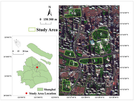
Figure 1.
Map of geographical location of study area. The numbers 1-6 in the figure represent the names of the sample blocks of urban PGSs in the study area. The names and composition profile of the blocks are listed in Table 2.
Table 2.
Study area profile.
2.2. Quantitative Index System Affecting Carbon Concentration Distribution
2.2.1. Selection and Quantification of Spatial Pattern Indices
A total of nine spatial pattern indices were selected to construct the index system. Among them, three-dimensional green biomass density, canopy density, and cohesion are the spatial structural indices of green spaces. In addition, arbors, shrubs, herbs, parkways, open land, and waterbody area ratio are the spatial composition indices of green spaces. The reasons for the selection of indices are as follows.
- Three-dimensional Green Biomass Density
Three-dimensional green biomass density (Gb) is the volume occupied by all green stems and leaves of plants in the space per square meter. Compared with the two-dimensional indices, it can show the level of ecological benefits of green space from a multi-level perspective [48]. According to the three-dimensional green volume model of Zhou, the three-dimensional green biomass density of trees was calculated on a plant-by-plant basis using the relationship equation between standing crown height and crown diameter [49]. Shrubs and herbs are ground cover plants. Their green biomass density is the product of the area occupied during scenario simulation modeling and their set height [50]. The sum of the green density of trees, shrubs, and grasses is the total Gb, and was calculated and counted in Excel2021 (Microsoft office, Redmon, WA, USA) and ArcGIS10.4 software (Esri, Redlands, CA, USA).
- 2.
- Canopy Density
Canopy density (CanopyD) is an important index reflecting the structure and density of the stand. It is often determined by the ratio of canopy projection area to woodland area [51]. Canopy densities mentioned in this study are all vertical canopy density. The canopy area of a single tree was calculated by using the canopy radius formula in ArcGIS to obtain the estimated canopy density [52].
- 3.
- Cohesion
The degree of patch agglomeration is an effective index to evaluate the connectivity of the spatial structure characteristics of the landscape [53]. The study chose the patch cohesion index (Co) to evaluate the connectivity of green landscape in the park. As the most dominant green landscape, trees and shrub patches were chosen to calculate the cohesion index in the whole, which was used to measure the natural state connectivity of the green space. As the distribution of each tree patch becomes more and more concentrated, the natural connectivity increases, and the patch cohesion index increases. Cohesion was calculated in Fragstats4.2 and its formula is [54]:
where i is the landscape type, j is the number of patches, n is the sum of patches in landscape type i, m is the sum of landscape types, is the area of the patches, is the perimeter of the patches, and A is the entire landscape area. 0 ≤ Cohesion ≤ 100.
- 4.
- Green space composition index
Discussing the correlation between green space compositions and CO2 concentration differentiation from the perspective of land use type may provide insight for later park green space planning. According to the research modeling, this study abstracted the internal space of the park into six types at the two-dimensional level: arboreal area, shrub area, herbs area, parkways, open land, and waterbody. The composition indices were expressed as the percentage of the area of each type in the total area, which were calculated statistically in ArcGIS software. All land use types are mutually exclusive, so the percentages of the six types add up to 100%.
2.2.2. Calculation and Analysis of Spatial Indices by Means of Unit Raster Statistics
This research examined the correlation between spatial morphological indices, microclimatic and biological indices at various scales to identify the spatial variation of CO2. Hence, ArcGIS software was employed to establish fishing nets to partition the study area of every park into several 20 m × 20 m grids. Regarding the setting of raster size, when exploring the landscape pattern indices, it is generally considered that 5–35 m is a suitable range of granularity for analysis, and the change of landscape aggregation with granularity is highly predictive [55,56,57]. In the studies of community-scale analysis of CO2 concentration distribution [30], three-dimensional green volume in urban parks [50], and plant canopy space and microclimate effects in residential green areas [58], the unit space was divided according to the size of 20 m × 20 m. In summary, this study extracted the coordinate range information of the study area from ArcGIS software to generate a matrix of points with the same spatial interval to form a unit space of 20 m × 20 m for calculating the indices. Through the above pre-processing method, the specific interpretation of each index is shown in Table 3.
Table 3.
Implications of spatial pattern indices.
2.2.3. Microclimate and Physical and Physiological Indices Influencing Carbon Cycle Interaction
CO2 concentration data in the Atmosphere module of ENVI-met5.2 was used to represent the distribution of CO2 concentration in PGSs. Since the most obvious differentiation of CO2 concentration occurs at 11 a.m. in the daytime, each unit space was taken as the statistical sample unit for standardization processing. The mean value of atmospheric CO2 concentration difference in unit space at 11 a.m. was calculated—namely, . —as the normalized CO2 concentration data, which represents the level of air CO2 concentration in this unit space.
The specific calculation method for is as follows:
where Ch is the original CO2 concentration of each grid at a certain height (h) obtained from simulation, h is the height of grids (h1 = 0.3 m, h2 = 1.5 m, h3 = 4.5 m, h4 = 7.5 m, h5 = 10.5 m), j is the serial number of the selected height and its maximum is 5, n is the amount of grids in each 20 × 20 unit space, and m is the amount of grids in each block.
According to the formula, the smaller is, the lower the CO2 concentration in the unit space is. < 0 indicates that the CO2 concentration in the unit space is lower than the average concentration in the block, and vice versa.
The mean values of other impact indices simulated by ENVI-met in each unit space were normalized. A total of eight indices simulated by ENVI-met software were selected to be added to the discussion of the interaction mechanism of spatial patterns affecting CO2 concentration. Microclimate indices affecting surface–air interaction, such as air temperature (AT), relative humidity (RH), wind speed (WS) and surface albedo (SA), were selected. Photosynthetically active radiation (PAR), turbulent kinetic energy (TKE), transpiration flux (VF), and stomatal resistance (SR) were the physical or biological indices associated with the photosynthetic response of vegetation. AT, RH, WS, and CO2 concentration were calculated in the same way. After calculating the difference of simulated points, the average value in the unit space was taken. SA does not need to consider the height, and the index was directly taken as the mean value in the unit space. PAR, TKE, VF, and SR are indices within the organism, so the mean values of the biological indices in the unit space were calculated after the data of five heights of each simulated point were added. The specific explanation of each index is shown in Table 4.
Table 4.
Implications of carbon cycle interaction mechanism influencing indices.
2.3. Study Methods
2.3.1. ENVI-Met Dynamic Simulation
ENVI-met5.0.2 software (developed by Michael Bruse, at the Bochum, German) was used to simulate the microclimate of PGSs. ENVI-met is a climate simulation software developed by the team of Bruse and Fleer in Germany, which creates a three-dimensional model of the study area to simulate its microclimate. In this study, the database in ENVI-met software can configure the composite structure of trees, shrubs, and herbs and modify the parameters of soil layer and water body according to the actual situation of urban park. The tree database is abundant, can be selected according to the tree species and growth rules. Canopy width, height, and other data of each tree species support users to modify the suitability according to local conditions.
The simulation date of this study was 21 June 2022, and the meteorological data were obtained from the meteorological station of Shanghai Hongqiao Airport on the Weather Underground website [59]. The initial input meteorological parameters and three-dimensional modeling parameters of the plot are shown in Table 5. With reference to the research on the photosynthetic characteristics and configuration of various dominant tree species in Shanghai [35,60], and combined with the distribution of each tree species, Platanus, Robinia, Cinnamomum, Privet, and Metasequoia were selected, respectively, and were constructed according to the actual landscape composition.
Table 5.
ENVI-met setting of basic environment values for scenario simulation.
Many scholars have used ENVI-met to conduct microclimate studies and verified the validity of the simulation results [61,62,63,64]. In this study, the simulation results of ENVI-met were compared with the observed values to verify the validation of the software on CO2 concentration. Fuxing Park, one of the research objects, was selected as the measured site, and 10 monitoring points were arranged (Figure 2). A CO2 real-time measuring instrument and a hand-held meteorological instrument were used to measure the meteorological indices and CO2 concentration at 1.5 m above the ground seven times at ten sites between 8 a.m. and 18 p.m. on 18 September 2022. Finally, the average value of seven measurements at each point was taken as the measured value of CO2 concentration at that point to verify the simulated data.
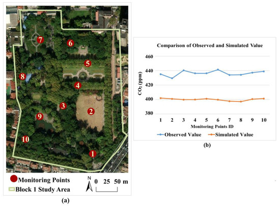
Figure 2.
Distribution of measuring points and measured values: (a) distribution map of field measuring points; (b) comparison of observed and simulated mean values at each point. The numbers 1–10 in the figure represent the selected on-site monitoring points.
Two verification methods, root mean square error (RMSE) and mean absolute percentage error (MAPE), were used to evaluate the deviation between simulated and measured values. Among them, RMSE measures the absolute deviation between simulated value and measured value. The lower the RMSE value is, the better the simulation accuracy is; otherwise, the worse it is. The relative size of deviation between simulated value and measured value measured by MAPE is generally believed to be less than 10%, indicating high accuracy of simulation prediction [65].
The RMSE value of CO2 concentration was 1.67 ppm and the MAPE was 8.4%. The RMSE of AT was 0.168 °C, and the MAPE was 7.01%. The RMSE value of RH was 0.699%, and the MAPE was 1.58%. Concerning the error value of the two verification methods of model in this study, it can be considered that ENVI-met simulation is able to predict CO2 concentration accurately.
2.3.2. BRT Machine Learning Model
The BRT model is a self-learning method based on categorical regression trees, developed by Elith et al. in 2008. It uses boosting techniques to fit multiple decision trees to determine the optimal model [66]. Compared with traditional regression models, the BRT model has strong adaptability to datasets and can process continuous data and classified data. In addition, the BRT model is not sensitive to multiple linearity and does not need to consider the multicollinearity problems faced by multiple linear regression analysis and can reflect the interaction between variables.
The BRT model in this study was executed using the dismo package of RStudio (Posit, Boston, Massachusetts, USA). The dependent variable was the atmospheric CO2 concentration after unit space standardization treatment (). The independent variables were the spatial indices of PGSs, microclimate, and physical and physiological indices after unit space standardization. The model parameters were set to tree complexity = 3, learning rate = 0.001, bag fraction = 0.5, and the data type was Gaussian distribution. The model extracted 50% of the data for analysis and 50% for training, and cross-validation was performed 10 times to estimate the number of optimal trees.
2.3.3. ME Curve and Fitted Scatter of the BRT Model
The output result of the BRT model scales the sum of relative influences of each variable to 100. The contribution ratio of each index can determine the importance of each independent variable indices to in unit space. The greater the value of the index contribution ratio, the greater the correlation with the dependent variable. The BRT model can also simulate the marginal effect (ME) of the independent variable, reflecting its contribution to the dependent variable in different intervals. It is necessary to determine the meaning represented by the ME curve in this study:
1. The fitted function of the Y-axis in the ME curve is the slope value of the total effect curve corresponding to the index and the dependent variable. When the ME curve showed a downward trend, the larger the index, the better the effect of reducing CO2 concentration; on the contrary, when the ME curve showed an upward trend, the greater the index, the worse the effect of reducing CO2 concentration.
2. The slope of the ME curve represents the degree of marginal utility change. When the absolute value of the slope of the ME curve is large, the marginal utility increases greatly. When the slope degree of ME curve changes greatly, such as from a sharp downward trend to a gentle one, the value of this inflection point may be a critical value for the index to play a role in reducing CO2 concentration.
When analyzing the ME curves of spatial indices and CO2 concentration, it will be of more help to combine with the fitted scatter plots. The meaning of the coordinate axes of the fitted scatter plot is the same as that of the ME curve. The Y-axis is the fitted function, and the X-axis is the value of the spatial indices. The meaning of the fitted scatter is as below.
1. When a certain spatial index in the fitted scatter plot is relatively evenly distributed on the X-axis and has a similar upward or downward trend to the ME curve, it can be confirmed that the nonlinear relationship of this ME curve is representative.
2. If a specific spatial index has only a few scattered points in a certain value interval of the X-axis, it implies that only a small number of samples have such spatial characteristics. If the ME curve of this spatial index fluctuates at this time, it is more likely to be caused by other indices.
3. Similarly, if the scattered points of a specific spatial index are too dense in a certain value interval of the X-axis, it may cause more fluctuation of the ME curve by excessive data volume. In this case, we will pay more attention to the trend of its overall change.
Through the combined analysis of these two types of figures, the statistical data characteristics of the spatial pattern of PGSs can be better understood so as to have a better investigation of the nonlinear relationship between spatial pattern indices and CO2 concentration.
2.3.4. Scatter Analysis of Spatial Pattern Indices and Carbon Cycle Interaction Indices
In the discussion, the relationships between spatial indices, microclimate indices, and physical and physiological indices were further discussed. When discussing the carbon cycle interaction process, we try to explore whether the difference of spatial indices is the driving force of the change in the carbon cycle interaction indices of PGSs. At the same time, the regularity of some plots with good carbon sink effect is obtained. Therefore, we selected some data with significant carbon sink effect and showed the potential relationship between the carbon cycle data through the scatter plot.
3. Results
3.1. Spatial and Temporal Distribution of CO2 Concentration
3.1.1. Variation of CO2 Concentration in Green Space
The difference between the carbon concentration of CO2 at 1.5 m at 6 a.m. and 11 a.m. for each simulation point was calculated and is presented in Figure 3. From the value of the legend, a negative value indicates that the CO2 concentration of the grid at 11 a.m. is lower than that at 6 a.m. A positive value means that the CO2 concentration on the grid at 11 a.m. is higher than that at 6 a.m. According to the comparison of aerial map and heat map in Figure 3 and Appendix Figure A1, Figure A2, Figure A3, Figure A4 and Figure A5, the absolute difference in CO2 between the two time passes within the park area is negative, showing that the CO2 concentration at 11 a.m. is lower than that at 6 a.m. in the morning. During this period, photosynthesis of green vegetation absorbs the CO2 in the atmosphere near the vegetation in PGSs, and the amount of photosynthetic absorption is greater than that released by respiration.
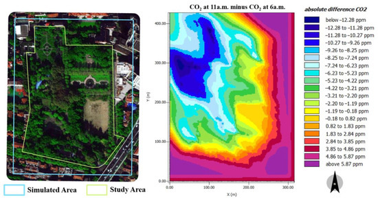
Figure 3.
Differentiation of CO2 concentration formed by photosynthesis of greenery in Block 1.
The regulations between green space and CO2 concentration can be indicated by the differentiation value of heat map. The photosynthetic rate in the area covered by trees is the highest during the five hours, and the absolute difference CO2 concentration reaches −5 ppm or even lower. The absolute difference CO2 concentration in the highly clustered tree communities is below −10 ppm. Large areas of grassland also reduce carbon concentrations during this period, with an absolute difference of −5 to 0 ppm. In the outer buffer zone, absolute difference CO2 concentrations increases by around 4 ppm between 6 a.m. and 11 p.m. Although the absolute difference of CO2 in some open fields in the study area is greater than 0, it also inhibits the increase in CO2 concentration compared with the increase in CO2 concentration in the peripheral buffer zone, which may be related to the CO2 absorption ability by bare soil.
To summarize, the area with high vegetation coverage has obvious spatial differentiation characteristics and becomes the low value interval of CO2 concentration distribution diurnally. To be more precise, PGSs function as a carbon sink in the diurnal period, transforming green patches with high CO2 concentration in the entire plot to low-carbon zones before the day starts.
3.1.2. The Hourly Change of PGSs Carbon Sequestration Capacity
In the simulation results of each block, a point with dense greening (G) coverage was selected, and a simulation point with bare (B) soil without any greening was selected. The difference of CO2 concentration between the two sites () was calculated. per hour represents the carbon sequestration effect of green space vegetation. The smaller the is, the greater the differentiation of CO2 concentration in PGSs, and the better the carbon sequestration effect of PGSs.
In terms of the overall changes of the six plots from 6 a.m. to 18 a.m., the of the greenery shows an overall trend of first decreasing and then increasing (Figure 4). According to the principle of photosynthesis, after receiving sunlight in the daytime, vegetation begins to carry out photosynthesis, and its ability to absorb CO2 is continuously strengthened. In this case, respiration gradually intensifies and produces more CO2 as raw material for photosynthesis, forming a positive feedback loop between photosynthesis and respiration that constantly promotes each other. As a result, the photosynthetic rate of green space increases gradually after the day begins. The photosynthesis effect of green space is the best between 10 a.m. and 12 a.m., and the difference of CO2 concentration is the greatest at 11 a.m. After 11 a.m., the positive feedback cycle between photosynthesis and respiration gradually weakens with the tilt of the solar altitude angle. Although the CO2 concentration in the greenery is still lower than that in the bare soil area, the carbon sink effect is gradually weakened.
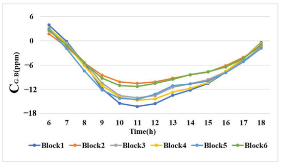
Figure 4.
Hourly change of in six blocks.
3.2. Analysis of Spatial Pattern Indices on the Reduction of Air CO2 Concentration
3.2.1. Contribution Ratio of Spatial Pattern Indices
BRT analysis results of atmospheric CO2 concentration () and spatial patterns indices after unit space standardization are shown in Table 6. For green space structural variables, Gb plays the most important role (19.44%). In the green space structural variables, Co (11.60%) and CanopyD (11.36%) both have a higher contribution ratio. In the green space composition variables, the contribution ratio of Ar is 18.90%, ranking first among green space composition indices. The contribution ratios of Hr and Pr ratio are 12.14% and 13.13%, respectively. After that, the ratios of Or (10.03%), Sr (2.86%), and Wr (0.53%) are successively followed.
Table 6.
Contribution ratios of spatial pattern indices.
3.2.2. Marginal Effect of Spatial Structural Indices
According to the results of BRT analysis, Gb contributes the most among all spatial pattern indices. Moreover, the ME curve largely illustrates the effect of PGSs on reducing CO2 concentration (Figure 5a). According to the ME curve, in the initial interval from zero to 0.1 m3/m2, the ME curve of Gb has an obvious downward trend, which is almost vertical, and rapidly approaches 0. When the Gb is between 0.1–0.25 m3/m2, the ME curve still has an obvious downward trend. After that, the ME curve shows a rising and then falling trend between 0.25–1 m3/m2. After 1 m3/m2, it is relatively smooth. In the range of 1.8–2.5 m3/m2, there is a small fluctuation that first drops and then rises. In general, Gb is always negatively correlated with , and the effect of reducing CO2 concentration is slowly enhanced with the increase in Gb.
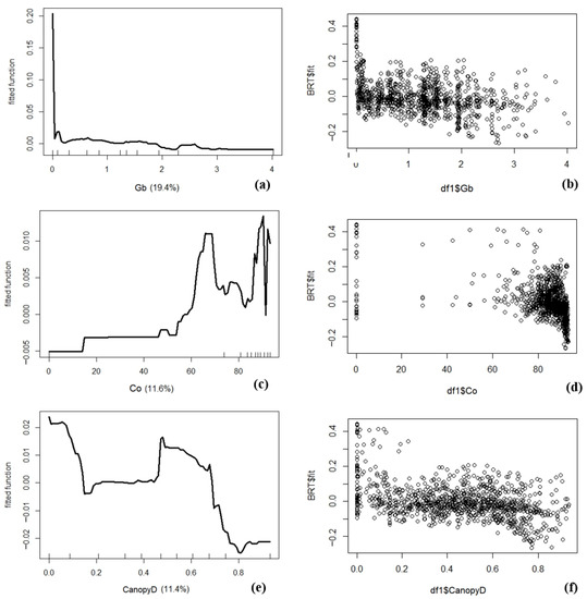
Figure 5.
ME curve and scatter distribution of spatial structural indices: (a) Gb ME curve; (b) Gb fitted scatter; (c) Co ME curve; (d) Co fitted scatter; (e) CanopyD ME curve; (f) CanopyD fitted scatter.
The regularity of Cohesion’s ME curve shows great fluctuation. Until Co is less than 65, greater Co is associated with greater CO2 concentration. Co is positively correlated with the carbon concentration distribution for grids containing less greenery that often have lower cohesion; that is, although the ecological agglomeration of patches increases, the CO2 concentration does not decrease significantly. Co and show a strong negative correlation between 65 and 75, and then the ME curve becomes flat. After Co to 83, the ME curve fluctuates greatly. Due to the influence of green biomass and other indices on CO2 concentration distribution, there is no significant correlation between the data changes. Co and CO2 concentration show a clear negative correlation overall in combination with the scatter distribution relationship (Figure 5d).
The ME curve of CanopyD shows two negative correlations between canopy density and CO2 concentration. Overall, the greater the canopy density, the better the effect of reducing CO2 concentration. When CanopyD is between 0 and 0.15, there is an obvious negative correlation between CanopyD and , which indicates that when trees are sparse, the increase in canopy shade area can reduce the CO2 concentration. When CanopyD is greater than 0.2 and less than 0.45, the ME curve changes gently and approaches the negative value of 0. When CanopyD increases from 0.2 to 0.4, the marginal benefit of reducing CO2 concentration is low. When CanopyD is about 0.45, the marginal effect rapidly increased to the maximum, and then the two show a negative correlation again. The marginal effect decreases to 0 when CanopyD is about 0.7, and the total effect on CO2 concentration is the maximum.
3.2.3. Marginal Effect of Spatial Compositional Indices
- The indices describing greenery areas
Among the green space composition indices, Ar, Hr, and Sr are negatively correlated with CO2 concentration (Figure 6). Ar is the index with the largest contribution ratio to the reduction of CO2 concentration among the spatial composition indices. There is a significant negative correlation between Ar and . The larger the arboreal area, the better the effect of reducing CO2 concentration. Ar reaches the maximum marginal effect at 52%, and then the marginal utility decreases significantly. Hr is also negatively correlated with . The larger the grassland area, the better the effect of reducing CO2 concentration. Its marginal benefit threshold is about 20%. Sr and CO2 concentration show an interactive relationship of first increasing and then decreasing. Its marginal effect threshold is about 10% and then presents a significant negative correlation.
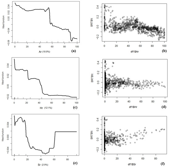
Figure 6.
ME curve and scatter distribution of indices describing greenery areas: (a) Ar ME curve; (b) Ar fitted scatter; (c) Hr ME curve; (d) Hr fitted scatter; (e) Sr ME curve; (f) Sr fitted scatter.
- 2.
- The indices describing non-greenery areas
Among the space compositional indices, Pr has the largest contribution among non-greenery indices. Pr has always shown a significant positive correlation with . The rise trend of the ME curve of Pr is the most obvious after 30%, and it also reaches 0 value during this rising trend. Pr with the best marginal benefit is 30%, and it is better to control the road area ratio below 30% in park planning aiming at reducing CO2 concentration. Open areas are generally located at entrances or large squares with good ventilation. Therefore, Or is negatively correlated with at the beginning. When Or is more than 65%, there is less greenery area. Currently, Or shows a positive correlation with , and the upward trend of the curve is steeper than the downward trend. The contribution of Wr to the reduction of CO2 concentration is the least. The total area ratio of waterbody is less than 5% in the six blocks, and over 92% of grids contain a water ratio of less than 5%. The contribution of Wr is only 0.5%, which has little effect on reducing CO2 concentration in the PGSs (Figure 7).
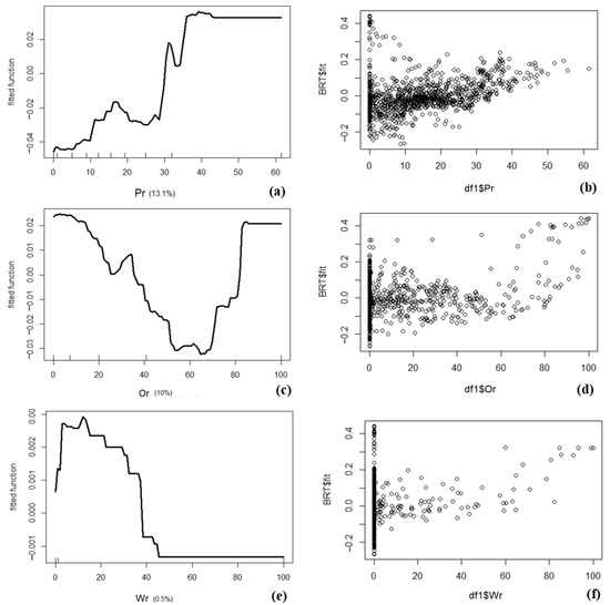
Figure 7.
ME curve and scatter distribution of indices describing non-greenery areas: (a) Pr ME curve; (b) Pr fitted scatter; (c) Or ratio ME curve; (d) Or fitted scatter; (e) Wr ME curve; (f) Wr fitted scatter.
3.3. The Influence of Indices Based on Carbon Cycle Interaction Mechanism
3.3.1. Contribution Ratio of Carbon Cycle Interaction Indices
, microclimate, and physical and physiological indices were analyzed by BRT. Results are shown in Table 7. Three microclimatic indices have the greatest influence on , which are WS (33.71%), AT (13.57%), and RH (12.45%). SA has a smaller impact (7.40%). Physical and physiological indices are arranged, respectively, as PAR (12.15%), SR (8.91%), VF (6.18%), and TKE (5.64%).
Table 7.
Contribution ratios of carbon cycle interaction indices.
3.3.2. Marginal Effect of Carbon Cycle Interaction Indices
The relationship between carbon cycle interaction indices and CO2 concentration can be obtained through the ME curve. In terms of microclimate indices (Figure 8), WS, AT, and RH have obvious associations to follow with CO2 concentration. The higher the WS and the higher AT, the higher the CO2 concentration. On the contrary, the higher the RH, the lower the CO2 concentration.
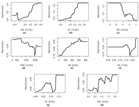
Figure 8.
ME curve of carbon cycle interaction indices: (a) WS; (b) AT; (c) RH; (d) PAR; (e) SR; (f) SA; (g) VF; (h) TKE.
In terms of biological indices, the contribution ratio of photosynthetic effective radiation to CO2 concentration is the highest, indicating that the main reason for the lower CO2 concentration in PGSs in diurnal period is the photosynthesis of plants. The higher the PAR before 2200 micro mol·m−2·m−1, the lower the CO2 concentration. At the same time, the plants reach their light saturation point at 2200 PAR value. The greater the SR, the more closed the stomata inside the plant. Gas exchange will not be able to take place well, and the higher the concentration of CO2 in the air will be. SA before 0.15 and after 0.17 shows a positive correlation with , and the ME curve of SA between 0.15 and 0.17 shows a negative correlation that may be related to the SA of urban green space, which is generally between 0.15 and 0.17 [67,68]. When the VF is above 0.06, the transpiration effect is small. Due to the lack of water, the stomata conductance of plants is small, and they cannot fully carry out photosynthesis. When the VF is greater than 0.11, there is too much water inside the plant, which may cause poor ventilation and hinder gas exchange. The TKE ME curve, which reflects the characteristics of atmospheric turbulence, shows a state of fluctuation, but the overall regularity has similarity with WS. The higher TKE is, the higher the CO2 concentration will be.
4. Discussion
4.1. Spatial Indices Differences Result in the Distribution of Carbon Cycle Interaction Indices
The unit spatial data of < −1 ppm, Gb > 1 m3/m2, Ar > 52%, and Hr < 20% were selected for further comparison. These data have a significant carbon sink effect. Investigating the correlation between spatial indices and the carbon cycle interaction indices within green areas demonstrates that the variance in spatial indices is the principal impetus for the alteration of microclimate and physical and physiological indices inside PGSs.
In Figure 9, the Gb data is divided into GB > 2.5 m3/m2, 2.5–1.5 m3/m2, and <1.5 m3/m2. Scatter plots visualize three grades of Gb, as well as the connections between the climatic environment indices and the physical and physiological indices. As can be seen from Figure 9a–d, Gb presents an obvious negative correlation with WS, AT, and SA. GB and RH show a significant positive correlation. Different levels of Gb are also related to the typical differentiation characteristics of microclimate indices and biological physiological indices. The internal space PGSs with high Gb usually has the following characteristics: lower WS, slightly lower AT, higher RH, and smaller SA of climate environmental indices. Similarly, the spatial differentiation of physical and physiological indices corresponding to unit space of high green density has the regularity of smaller PAR, larger SR, smaller VF, and smaller TKE in internal space.
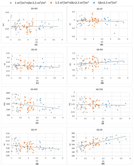
Figure 9.
Scatter plot of the interaction between Gb and carbon cycle interaction indices: (a) Gb and WS (b) Gb and AT; (c) Gb and SA; (d) Gb and RH; (e) Gb and PAR; (f) Gb and TKE; (g) Gb and VF; (h) Gb and SR.
4.2. Variation of Spatial Indices on CO2 Concentration
With the data selected in Section 4.1, the influences of Gb, Ar, CanopyD, and Co on CO2 concentration were further analyzed. In Figure 10, the four indices are negatively correlated to . In other words, with the increase in the values of these four indices, the overall trend is that CO2 concentration decreases, and the carbon sink effect is better. Moreover, the data performance of the four indices was graded to find the corresponding variation rules of CO2 concentration in different spatial levels. Gb takes 1.5 m3/m2 and 2.5 m3/m2 as the boundary value of data division. Ar grades of 70% and 90% are interval data. CanopyD uses 0.6 and 0.7 as classification boundary data. The data of Co are 86% and 90% interval data. The distribution and differentiation of different grade intervals of spatial indices and CO2 concentration are as follows: the higher the grades of spatial indices, the lower the corresponding value of CO2 concentration.
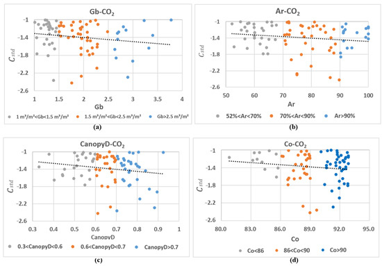
Figure 10.
Scatter plot of the interaction between spatial indices and Cstd: (a) Gb and Cstd; (b) Ar and Cstd; (c) CanopyD and Cstd; (d) Co and Cstd.
4.3. The Interaction of Microclimate and Environment Indices, Physical and Physiological Indices, and CO2 Concentration
The study continued to explore the internal atmospheric cycling process of CO2 concentration change between PGSs with high carbon sink capacity and PGSs with low carbon sink capacity. Two groups of data, < −1 ppm and > 1 ppm, with typical differences were selected to analyze the correlation between microclimate indices and physical and physiological indices. In terms of the overall characteristics, the PAR, SR, VF, and TKE are larger when the WS is smaller. Meanwhile, compared with the low carbon sink space, the WS, AT, and SA corresponding to < −1 ppm are smaller, and RH is relatively small. The series comparison of WS relatively affects the physical and biological indices PAR, SR, TKE, and VF, and there is a significant difference in the value range. In Figure 11a–d, when WS ranges from −0.25 to 0 m/s, PAR, VF, and TKE reach their maximum values; when WS is less than −0.25 m/s, the activity of biological indices decreases slightly. In Figure 11e–g, under the condition of high carbon concentration, the biological activity of some extremely high temperature and extremely low humidity spaces do not reach the peak. The SA between 0.17 and 0.25 and VF and other biological indices also show that the larger the SA, the smaller the biological indices. Because SA of the space with higher greenery coverage is between 0.17 and 0.2, the material exchange activity of the vegetated area is greater (Figure 11h).
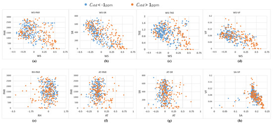
Figure 11.
Scatter plot of the interaction relationship between microclimate indices and physical-physiological indices: (a) WS and PAR; (b) WS and SR; (c) WS and TKE; (d) WS and VF; (e) RH and PAR; (f) AT and PAR; (g) AT and SR (h) SA and VF.
4.4. Strategies to Improve the Carbon Sink of Urban Park
Through the analysis of the marginal effect threshold between the spatial form description indices and carbon concentration of park green space, the research can provide the quantitative control requirements for policymaking in terms of the spatial pattern indices of PGSs. In green space management aiming for carbon reduction, the green biomass density is more appropriate at 1–2.5 m3/m2. The canopy density of low-carbon green open space is best at about 0.7, the arboreal area ratio should be around 52%, and the grassland area ratio is about 20%, and would benefit if the area ratio of parkways was controlled below 30%.
The effects of the internal composition and structural indices of PGSs on carbon storage are non-linear. Therefore, there are interactive effects and constraints on the spatial indices affecting carbon absorption capacity. For example, the green amount is a three-dimensional pattern index reflecting the amount of green biomass. In addition, most studies have shown that increasing the amount of green biomass is crucial for the overall carbon sequestration capacity of the city [11,14,43]. This study found that there is a restrictive relationship between PAR and Gb. According to Figure 8d, before reaching the light saturation point, the higher the value of PAR, the more promoting the energy of carbon absorption. Figure 12a shows that when Gb is less than 1.5 m3/m2, the Gb increases, and the PAR increases further. The increase in PAR represents the enhancement of light energy utilization efficiency. When Gb is greater than 1.5 m3/m2, PAR reduces when Gb is further increased, and the light energy utilization efficiency is also reduced. The efficient usage of PAR is the key to increasing carbon sequestration capacity. The correlation between Gb and CanopyD also shows a quadratic curve variation trend. When Gb increases and vegetation is dense, CanopyD tends to slow down with the increase in green amount (Figure 12b). Their associated characteristics will affect the effective light utilization of the PAR. After the green biomass reaches a certain value, the vegetation is too dense, the PAR will decrease, and the vegetation cannot be fully illuminated, thus affecting the reduction of its carbon sink efficiency. Therefore, in the process of improving the green amount of PGSs, it is necessary to consciously control other spatial indices within the appropriate interval and to ensure that the greening receives sufficient light and creates the appropriate conditions for the occurrence of physical and biological processes. For the design and management of PGSs, controlling the appropriate dense planting interval of arbor patches to ensure sufficient light and rationally matching the relationship between trees and grassland landscape configuration can lead to a better carbon sequestration effect than only pursuing the increase in green amount.
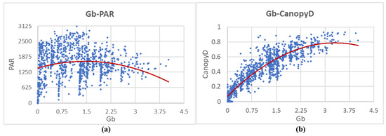
Figure 12.
Scatter plot of the relationship between Gb, PAR, and CanopyD: (a) Gb and PAR; (b) Gb and CanopyD.
4.5. Characteristics and Limitations of the Study
The Envi-met software was used to simulate the CO2 concentration distribution data, considering the biological complex diversity inside the actual site. BRT machine learning method was adopted to quantify the influence degree and trend characteristics of each index on CO2 concentration. In particular, the interactive effects of the carbon cycle in PGSs within the site were discussed innovatively. However, the study was abstract in its modeling. For example, only five species of typical Shanghai countryside tree species are selected. No further subdivision of herbs and shrub types was conducted, and the same height attribute was uniformly set. Although different types of soil were set according to the actual site in the scenario simulation, the main object of the study was the spatial patterns of PGSs, so the possible influence of soil respiration was not discussed.
Future studies can be explored on a larger spatiotemporal scale. This study only discussed the contribution degree and interaction mechanism of spatial morphology to CO2 concentration from a time cross-section. The sun’s altitude varies throughout the day; the same location and the same spatial form will receive different intensities of light at different times, thus affecting the photosynthetic efficiency of PGSs. On the other hand, deciduous trees alter their biomass during the year, especially some common tree species in Shanghai such as sycamores and acacia. In terms of space, this study simulated PGSs as an isolated green space patch. Although this reduces the influence of variables of human traffic activities, it can be considered to embed PGSs into the street scale in subsequent studies to explore the carbon sink effect of PGSs in different urbanization backgrounds.
5. Conclusions
In this paper, Envi-met software was used to simulate the distribution of CO2 concentration in typical PGSs. Through quantitative and qualitative methods, this study analyzed the interactive influence and carbon reduction mechanism between the spatial morphology and structure characteristics of PGSs and CO2 concentration to provide a reasonable planning path for the low-carbon patterns of PGSs.
PGSs act as carbon sinks in the diurnal period. During the morning hours of 10 a.m.−12 a.m. on a typical summer day, green space has a substantial capacity to take in CO2. The study observed the greatest disparity in CO2 concentration within the PGSs at 11 a.m. through simulation. Gb, Ar, Hr, Pr, CanopyD, and other spatial indices have the greatest effect on the variation of CO2 concentration distribution, respectively. The proportion of greenery, such as Gb and CanopyD, has a negative correlation with CO2 concentration, while the Pr and Or have a positive correlation with CO2 concentration. The waterbody in PGSs has little effect on CO2 concentration. The WS has the greatest influence on the carbon cycle, thus affecting the changes in CO2 concentration, and the role of microclimate is more significant than that of physical and physiological indices.
Furthermore, the greenery in parks adjusts air CO2 concentration through photosynthesis and forms an area with decreased WS and appropriate AT and RH due to its spatial arrangements. This is a vital component in the process of the microclimate influencing the spread of CO2 concentration. A suitable microclimate environment enables the plant to accelerate photosynthesis and other biological physiological reactions.
Author Contributions
Y.J.: conceptualization, methodology, supervision, writing—original draft, writing—review and editing. Y.L.: writing—original draft, methodology, software, investigation, formal analysis. Y.S.: validation, software, investigation. X.L.: validation, writing—review and editing. All authors have read and agreed to the published version of the manuscript.
Funding
This research study was funded by the National Natural Science Foundation of China project (grant numbers 51878279 and 51878418). The authors would like to thank the editor and the anonymous reviewers for their helpful comments.
Data Availability Statement
No data were used for the research described in the article.
Conflicts of Interest
The authors declare no conflict of interest.
Appendix A

Figure A1.
Differentiation of CO2 concentration formed by photosynthesis of greenery in Block 2.
Figure A1.
Differentiation of CO2 concentration formed by photosynthesis of greenery in Block 2.


Figure A2.
Differentiation of CO2 concentration formed by photosynthesis of greenery in Block 3.
Figure A2.
Differentiation of CO2 concentration formed by photosynthesis of greenery in Block 3.


Figure A3.
Differentiation of CO2 concentration formed by photosynthesis of greenery in Block 4.
Figure A3.
Differentiation of CO2 concentration formed by photosynthesis of greenery in Block 4.


Figure A4.
Differentiation of CO2 concentration formed by photosynthesis of greenery in Block 5.
Figure A4.
Differentiation of CO2 concentration formed by photosynthesis of greenery in Block 5.


Figure A5.
Differentiation of CO2 concentration formed by photosynthesis of greenery in Block 6.
Figure A5.
Differentiation of CO2 concentration formed by photosynthesis of greenery in Block 6.

References
- IPCC. IPCC Sixth Assessment Report. Available online: https://www.ipcc.ch/reports/ (accessed on 20 March 2023).
- Carretero, E.M.; Moreno, G.; Duplancic, A.; Abud, A.; Vento, B.; Jauregui, J.A. Urban forest of Mendoza (Argentina): The role of Morus alba (Moraceae) in carbon storage. Carbon Manag. 2017, 8, 237–244. [Google Scholar] [CrossRef]
- Velasco, E.; Roth, M.; Norford, L.; Molina, L.T. Does urban vegetation enhance carbon sequestration? Landsc. Urban Plan. 2016, 148, 99–107. [Google Scholar] [CrossRef]
- Dorendorf, J.; Eschenbach, A.; Schmidt, K.; Jensen, K. Both tree and soil carbon need to be quantified for carbon assessments of cities. Urban For. Urban Green. 2015, 14, 447–455. [Google Scholar] [CrossRef]
- Luo, Y.; Zhang, D.; Zhang, L.; Chen, X. Study on selection and collocation of urban greening tree species under dual carbon goal—A case study of Shanghai Expo Park. Landsc. Archit. Acad. J. 2022, 39, 25–32. (In Chinese) [Google Scholar]
- Baraldi, R.; Chieco, C.; Neri, L.; Facini, O.; Rapparini, F.; Morrone, L.; Rotondi, A.; Carriero, G. An integrated study on air mitigation potential of urban vegetation: From a multi-trait approach to modeling. Urban For. Urban Green. 2019, 41, 127–138. [Google Scholar] [CrossRef]
- Baró, F.; Chaparro, L.; Gómez-Baggethun, E.; Langemeyer, J.; Nowak, D.J.; Terradas, J. Contribution of ecosystem services to air quality and climate change mitigation policies: The case of urban forests in Barcelona, Spain. Ambio 2014, 43, 466–479. [Google Scholar] [CrossRef]
- Sun, Y.; Xie, S.; Zhao, S. Valuing urban green spaces in mitigating climate change: A city-wide estimate of aboveground carbon stored in urban green spaces of China’s Capital. Global Chang. Biol. 2019, 25, 1717–1732. [Google Scholar] [CrossRef]
- Zhang, G.; Xing, L.; Zhang, L.; Zhong, Q.; Yi, Y. Summary on the monitoring methods of carbon sequestration in urban green space. Landsc. Archit. Acad. J. 2022, 39, 4–9+49. (In Chinese) [Google Scholar]
- Idso, S.B.; Idso, C.D.; Balling, R.C. Seasonal and diurnal variations of near-surface atmospheric CO2 concentration within a residential sector of the urban CO2 dome of Phoenix, AZ, USA. Atmos. Environ. 2002, 36, 1655–1660. [Google Scholar] [CrossRef]
- Shen, G.; Wang, Z.; Liu, C.; Han, Y. Mapping aboveground biomass and carbon in Shanghai’s urban forest using Landsat ETM+ and inventory data. Urban For. Urban Green. 2020, 51, 126655. [Google Scholar] [CrossRef]
- Sallustio, L.; Quatrini, V.; Geneletti, D.; Corona, P.; Marchetti, M. Assessing land take by urban development and its impact on carbon storage: Findings from two case studies in Italy. Environ. Impact Assess. Rev. 2015, 54, 80–90. [Google Scholar] [CrossRef]
- Zhang, C.; Wang, L.; Song, Q.; Chen, X.; Gao, H.; Wang, X. Biomass carbon stocks and dynamics of forests in Heilongjiang Province from 1973 to 2013. China Environ. Sci. 2018, 38, 4678–4686. [Google Scholar] [CrossRef]
- Tsedeke, R.E.; Dawud, S.M.; Tafere, S.M. Assessment of carbon stock potential of parkland agroforestry practice: The case of Minjar Shenkora; North Shewa, Ethiopia. Environ. Syst. Res. 2021, 10, 1–11. [Google Scholar] [CrossRef]
- Hou, H.; Zhang, S.; Ding, Z.; Wang, Y.; Yang, Y.; Guo, S. Temporal variation of near-surface CO2 concentrations over different land uses in Suzhou City. Environ. Earth Sci. 2016, 75, 1197. [Google Scholar] [CrossRef]
- Pan, C.; Zhu, X.; Wei, N.; Zhu, X.; She, Q.; Jia, W.; Liu, M.; Xiang, W. Spatial variability of daytime CO2 concentration with landscape structure across urbanization gradients, Shanghai, China. Clim. Res. 2016, 69, 107–116. [Google Scholar] [CrossRef]
- Järvi, L.; Havu, M.; Ward, H.C.; Bellucco, V.; McFadden, J.P.; Toivonen, T.; Heikinheimo, V.; Kolari, P.; Riikonen, A.; Grimmond, C.S.B. Spatial Modeling of Local-Scale Biogenic and Anthropogenic Carbon Dioxide Emissions in Helsinki. J. Geophys. Res. Atmos. 2019, 124, 8363–8384. [Google Scholar] [CrossRef]
- Li, Y.; Gao, J.; Dong, S.; Zheng, J.; Jia, X. Study of CO2 emissions from traffic and CO2 sequestration by vegetation based on eddy covariance flux measurements in suburb of Beijing, China. Pol. J. Environ. Stud. 2020, 29, 727–738. [Google Scholar] [CrossRef]
- Hwang, K.; Papuga, S.A. COVID-19 pandemic underscores role of green space in urban carbon dynamics. Sci. Total Environ. 2023, 859, 160249. [Google Scholar] [CrossRef]
- Park, C.; Schade, G.W. Anthropogenic and biogenic features of long-term measured CO2 flux in north downtown Houston, Texas. J. Environ. Qual. 2016, 45, 253–265. [Google Scholar] [CrossRef]
- Salem, M.; Almuzaini, R.; Kishawi, Y. The impact of road transport on CO2 atmospheric concentrations in Gaza City (Palestine), and urban vegetation as a mitigation measure. Pol. J. Environ. Stud. 2017, 26, 2175–2188. [Google Scholar] [CrossRef]
- Ueyama, M.; Ando, T. Diurnal, weekly, seasonal, and spatial variabilities in carbon dioxide flux in different urban landscapes in Sakai, Japan. Atmos. Chem. Phys. 2016, 16, 14727–14740. [Google Scholar] [CrossRef]
- Vaccari, F.P.; Gioli, B.; Toscano, P.; Perrone, C. Carbon dioxide balance assessment of the city of Florence (Italy), and implications for urban planning. Landsc. Urban Plan. 2013, 120, 138–146. [Google Scholar] [CrossRef]
- Sage, R.F.; Kubien, D.S. The temperature response of C3 and C4 photosynthesis. Plant Cell Environ. 2007, 30, 1086–1106. [Google Scholar] [CrossRef] [PubMed]
- Salvucci, M.E.; Crafts-Brandner, S.J. Mechanism for deactivation of Rubisco under moderate heat stress. Physiol. Plant. 2004, 122, 513–519. [Google Scholar] [CrossRef]
- Meili, N.; Manoli, G.; Burlando, P.; Carmeliet, J.; Chow, W.T.; Coutts, A.M.; Roth, M.; Velasco, E.; Vivoni, E.R.; Fatichi, S. Tree effects on urban microclimate: Diurnal, seasonal, and climatic temperature differences explained by separating radiation, evapotranspiration, and roughness effects. Urban For. Urban Green. 2021, 58, 126970. [Google Scholar] [CrossRef]
- Mitchell, L.E.; Lin, J.C.; Bowling, D.R.; Pataki, D.E.; Strong, C.; Schauer, A.J.; Bares, R.; Bush, S.E.; Stephens, B.B.; Mendoza, D.; et al. Long-term urban carbon dioxide observations reveal spatial and temporal dynamics related to urban characteristics and growth. Proc. Natl. Acad. Sci. USA 2018, 115, 2912–2917. [Google Scholar] [CrossRef]
- Ward, H.; Kotthaus, S.; Grimmond, C.; Bjorkegren, A.; Wilkinson, M.; Morrison, W.; Evans, J.; Morison, J.; Iamarino, M. Effects of urban density on carbon dioxide exchanges: Observations of dense urban, suburban and woodland areas of southern England. Environ. Pollut. 2015, 198, 186–200. [Google Scholar] [CrossRef]
- He, C.; Li, J.; Guo, M.; Wang, Y.; Chen, C. Changes of leaf photosynthetic characteristics and water use efficiency along tree height of 4 tree species. Acta Ecol. Sin. 2008, 28, 3008–3016. (In Chinese) [Google Scholar]
- Zhu, X.-H.; Lu, K.-F.; Peng, Z.-R.; He, H.-D.; Xu, S.-Q. Spatiotemporal variations of carbon dioxide (CO2) at urban neighborhood scale: Characterization of distribution patterns and contributions of emission sources. Sustain. Cities Soc. 2022, 78, 103646. [Google Scholar] [CrossRef]
- Prentice, I.C.; Dong, N.; Gleason, S.M.; Maire, V.; Wright, I.J. Balancing the costs of carbon gain and water transport: Testing a new theoretical framework for plant functional ecology. Ecol. Lett. 2014, 17, 82–91. [Google Scholar] [CrossRef]
- Xiong, D.; Yu, T.; Zhang, T.; Li, Y.; Peng, S.; Huang, J. Leaf hydraulic conductance is coordinated with leaf morpho-anatomical traits and nitrogen status in the genus Oryza. J. Exp. Bot. 2015, 66, 741–748. [Google Scholar] [CrossRef]
- Wang, L.; Hu, Y.; Qin, J.; Gao, K.; Huang, J. Carbon fixation and oxygen production of 151 plants in Shanghai. J. Huazhong Agric. Univ. 2007, 26, 399–401. (In Chinese) [Google Scholar] [CrossRef]
- Anderson, M.C.; Kustas, W.P.; Norman, J.M. Upscaling and downscaling—a regional view of the soil-plant-atmosphere continuum. Agron. J. 2003, 95, 1408–1423. [Google Scholar] [CrossRef]
- Shao, Y.; Li, J.; Li, E.; Zhuang, J. Photosynthetic and transpiration characteristics of eight deciduos broad-leaved trees in summer in Shanghai. J. Northwest For. Univ. 2015, 30, 30–38. (In Chinese) [Google Scholar] [CrossRef]
- Xu, X.; Fang, J.; Zhang, Y. Analysis and research progress on the carbon fixation capacity of garden green space. J. Anhui Agric. Sci. 2017, 45, 58–62. [Google Scholar] [CrossRef]
- Xue, H.; Tang, H.; Li, Y.; Li, X.; Guo, J.; Ma, J. Regulation service of main greening tree soecies in Beijing. J. Beijing Norm. Univ. Nat. Sci. 2018, 54, 517–524. (In Chinese) [Google Scholar] [CrossRef]
- Zhang, J.; Shi, Y.; Zhu, Y.; Liu, E.; Li, M.; Zhou, J.; Li, J. The photosynthetic carbon fixation characteristics of common tree species in northern Zhejiang. Acta Ecol. Sin. 2013, 33, 1740–1750. (In Chinese) [Google Scholar] [CrossRef]
- Wang, Z. Research on vegetation quantity and carbon-fixing and oxygen-releasing effects of Fuzhou botanical garden. Chin. Landsc. Archit. 2010, 26, 1–6. (In Chinese) [Google Scholar] [CrossRef]
- Godwin, C.; Chen, G.; Singh, K.K. The impact of urban residential development patterns on forest carbon density: An integration of LiDAR, aerial photography and field mensuration. Landsc. Urban Plan. 2015, 136, 97–109. [Google Scholar] [CrossRef]
- Liu, M.; Zhu, X.; Pan, C.; Chen, L.; Zhang, H.; Jia, W.; Xiang, W. Spatial variation of near-surface CO2 concentration during spring in Shanghai. Atmos. Pollut. Res. 2016, 7, 31–39. [Google Scholar] [CrossRef]
- Yin, L.; Hang, T.; Xu, Y. Research on carbon sink performance of blue-green landscape spaces in the Wuhan garden expo park. S. Archit. 2020, 3, 41–48. (In Chinese) [Google Scholar] [CrossRef]
- Fan, Y.; Wei, F. Contributions of natural carbon sink capacity and carbon neutrality in the context of net-zero carbon cities: A case study of Hangzhou. Sustainability 2022, 14, 2680. [Google Scholar] [CrossRef]
- Wang, M.; Zhu, W. The impact of urban green space on carbon neutrality and spatial characteristics: A case study of Huangpu district in Shanghai. Landsc. Archit. Acad. J. 2021, 38, 11–18. (In Chinese) [Google Scholar] [CrossRef]
- Zhao, Y.; Kan, L.; Che, S. A preliminary study about common garden plants’ effect of carbon fixation and oxygen release in Shanghai’s community and optimal arrangement. J. Shanghai Jiaotong Univ. Agric. Sci. 2014, 32, 45–53. [Google Scholar] [CrossRef]
- Gao, Y.; Lee, X.; Liu, S.; Hu, N.; Wei, X.; Hu, C.; Liu, C.; Zhang, Z.; Yang, Y. Spatiotemporal variability of the near-surface CO2 concentration across an industrial-urban-rural transect, Nanjing, China. Sci. Total Environ. 2018, 631–632, 1192–1200. [Google Scholar] [CrossRef]
- Hutyra, L.R.; Duren, R.; Gurney, K.R.; Grimm, N.; Kort, E.A.; Larson, E.; Shrestha, G. Urbanization and the carbon cycle: Current capabilities and research outlook from the natural sciences perspective. Earth’s Future 2014, 2, 473–495. [Google Scholar] [CrossRef]
- Zhou, H.; Tao, G.; Yan, X.; Sun, J.; Wu, Y. A review of research on the urban thermal environment effects of green quantity. Chin. J. Appl. Ecol. 2020, 31, 2804–2816. (In Chinese) [Google Scholar] [CrossRef]
- Zhou, J.; Sun, T. Study on remote sensing model of three-dimensional green biomass and the estimation of environmental benefits of greenery. Remote Sens. Environ. 1995, 10, 162–174. [Google Scholar] [CrossRef]
- Yang, Y.; Hu, X.; Jin, X.; Yang, C.; Su, D. The influence of three-dimensional green biomass spatial distribution on cooling and humidifying effect of plant community in summer: Taking the park green space of Huaihua City as an example. J. Hunan Agric. Univ. Nat. Sci. 2022, 48, 181–189. (In Chinese) [Google Scholar] [CrossRef]
- Wang, X.; Teng, M.; Huang, C.; Zhou, Z.; Chen, X.; Xiang, Y. Canopy density effects on particulate matter attenuation coefficients in street canyons during summer in the Wuhan metropolitan area. Atmos. Environ. 2020, 240, 117739. [Google Scholar] [CrossRef]
- Fiala, A.C.S.; Garman, S.L.; Gray, A.N. Comparison of five canopy cover estimation techniques in the western Oregon Cascades. For. Ecol. Manag. 2006, 232, 188–197. [Google Scholar] [CrossRef]
- Chen, M.; Dai, F. The influence of urban green spaces on thermal environment based on morphological spatial pattern analysis. Ecol. Environ. Sci. 2021, 30, 125–134. [Google Scholar] [CrossRef]
- Jiang, Y.; Huang, J. Quantitative analysis of mitigation effect of urban blue-green spaces on urban heat island. Resour. Environ. Yangtze Basin 2022, 31, 2060–2072. (In Chinese) [Google Scholar]
- Cui, Y.; Dong, B.; Wei, H.; Xu, W.; Yang, F.; Peng, L.; Fang, L.; Wang, Y. Granularity effect of landscape index at the county scale. J. Zhejiang AF Univ. 2020, 37, 778–786. (In Chinese) [Google Scholar] [CrossRef]
- Meng, N.; Han, B.; Wang, H.; Lu, F.; Xu, C.; Ouyang, Z. Study on the evolution of urban ecosystem patterns in Macao. Acta Ecol. Sin. 2018, 38, 6442–6451. (In Chinese) [Google Scholar] [CrossRef]
- Zhu, M.; Pu, L.; Li, J. Effects of varied remote sensor spatial resolution and grain size on urban landscape pattern analysis. Acta Ecol. Sin. 2008, 28, 2753–2763. (In Chinese) [Google Scholar] [CrossRef]
- Li, Y.-H.; Wang, J.-J.; Chen, X.; Sun, J.-L.; Zeng, H. Effects of green space vegetation canopy pattern on the microclimate in residential quarters of Shenzhen City. Chin. J. Appl. Ecol. 2011, 22, 343–349. (In Chinese) [Google Scholar] [CrossRef]
- WeatherUnderground. Meteorological Data from the Meteorological Station of Shanghai Hongqiao Airport on June 21, 2022. Available online: https://www.wunderground.com (accessed on 21 June 2022).
- Yang, C.; Wang, Y. Vegetation arrangement of the recreational lawn space of urban park in Shanghai. J. Shanghai Jiaotong Univ. Agric. Sci. 2012, 30, 28–33. (In Chinese) [Google Scholar] [CrossRef]
- Jiang, Y.; Han, X.; Shi, T.; Song, D. Microclimatic impact analysis of multi-dimensional indicators of streetscape fabric in the medium spatial zone. Int. J. Environ. Res. Public Health 2019, 16, 952. [Google Scholar] [CrossRef]
- Jiang, Y.; Huang, J.; Shi, T.; Li, X. Cooling island effect of blue-green corridors: Quantitative comparison of morphological impacts. Int. J. Environ. Res. Public Health 2021, 18, 11917. [Google Scholar] [CrossRef]
- Tsoka, S.; Tsikaloudaki, A.; Theodosiou, T. Analyzing the ENVI-met microclimate model’s performance and assessing cool materials and urban vegetation applications–A review. Sustain. Cities Soc. 2018, 43, 55–76. [Google Scholar] [CrossRef]
- Zhu, Y.; Xie, W.; Huang, H. Modeling sensible flux and latene flux in Heihe and boreal forests based on a 3D ENVI-met model. J. Zhejiang AF Univ. 2018, 35, 440–452. [Google Scholar] [CrossRef]
- Chai, T.; Draxler, R.R. Root mean square error (RMSE) or mean absolute error (MAE)?—Arguments against avoiding RMSE in the literature. Geosci. Model Dev. 2014, 7, 1247–1250. [Google Scholar] [CrossRef]
- Elith, J.; Leathwick, J.R.; Hastie, T. A working guide to boosted regression trees. J. Anim. Ecol. 2008, 77, 802–813. [Google Scholar] [CrossRef]
- Feng, Y.; Feng, H. TM data retrieval and analysis of Beijing area surface albedo. Sci. Surv. Mapp. 2012, 37, 164–166. [Google Scholar] [CrossRef]
- Hao, W.; Yu, H.; Wang, H.; Zhou, C.; Zhang, F.; Tian, Y.; Jia, X.; Zha, T. Dynamics of surface albedo and its controlling factors in Beijing Olympic Forest Park. Chin. J. Ecol. 2019, 38, 427–435. [Google Scholar] [CrossRef]


Disclaimer/Publisher’s Note: The statements, opinions and data contained in all publications are solely those of the individual author(s) and contributor(s) and not of MDPI and/or the editor(s). MDPI and/or the editor(s) disclaim responsibility for any injury to people or property resulting from any ideas, methods, instructions or products referred to in the content. |
© 2023 by the authors. Licensee MDPI, Basel, Switzerland. This article is an open access article distributed under the terms and conditions of the Creative Commons Attribution (CC BY) license (https://creativecommons.org/licenses/by/4.0/).