Individual Tree Aboveground Biomass Estimation Based on UAV Stereo Images in a Eucalyptus Plantation

Abstract

As one of the three fastest-growing tree species in the world, eucalyptus grows rapidly, with a monthly growth rate of up to 1 m and a maximum annual growth rate of up to 10 m. Therefore, ways to accurately and quickly obtain the aboveground biomass (AGB) of eucalyptus in different growth stages at a low cost are the foundation of achieving eucalyptus growth-change monitoring and precise management. Although Light Detection and Ranging (LiDAR) can achieve high-accuracy estimations of individual eucalyptus tree biomasses, the cost of data acquisition is relatively high. While the AGB estimation accuracy of high-resolution images may be affected by a lack of forest vertical structural information, stereo images obtained using unmanned aerial vehicles (UAVs) can not only provide horizontal structural information but also vertical structural information through derived point data, demonstrating strong application potential in estimating the biomass of eucalyptus plantations. To explore the potential of UAV stereo images for estimating the AGB of individual eucalyptus trees and further investigate the impact of stereo-image-derived features on the construction of biomass models, in this study, UAVs equipped with consumer-grade cameras were used to obtain multitemporal stereo images. Different features, such as spectral features, texture, tree height, and crown area, were extracted to estimate the AGB of individual eucalyptus trees of five different ages with three algorithms. The different features extracted based on the UAV images had different effects on estimating AGB in individual eucalyptus trees. By estimating eucalyptus AGB using only spectrum features, we found that tree height had the greatest impact, with its R² value increasing by 0.28, followed by forest age. Other features, such as spectrum, texture, and crown area, had relatively small effects. For the three algorithms, the estimation accuracy of the CatBoost algorithm was the highest, with an R² ranging from 0.65 to 0.90, and the normalized root-mean-square error (NRMSE) ranged from 0.08 to 0.15. This was followed by the random forest algorithm. The ridge regression algorithm had the lowest accuracy, with an R² ranging from 0.34 to 0.82 and an NRMSE value ranging from 0.11 to 0.21. The AGB model that we established with forest age, TH, crown area, and HOM-B feature variables using the CatBoost algorithm had the best estimation accuracy, with an R² of 0.90 and an NRMSE of 0.08. The results indicated that accurately estimating the AGB of individual eucalyptus trees can be achieved based on stereo images obtained using UAVs equipped with affordable, consumer-grade cameras. This paper can provide methodological references and technical support for estimating forest biomass, carbon storage, and other structural parameters based on UAV images.

1. Introduction

Eucalyptus plantations are mostly distributed in tropical and subtropical regions, especially in Brazil, India, and China [1]. They have good woody properties and are the most important source of short fibers in pulp and paper production [2]. They also grow rapidly, with a monthly growth rate of up to 1 m and a maximum annual growth rate of up to 10 m. For fast-growing eucalyptus plantations, ways to accurately and quickly obtain the aboveground biomass (AGB) value of eucalyptus in different growth stages at a low cost are the foundation of achieving eucalyptus growth-change monitoring and precise management, which are of great significance for the planning, management, and policy formulation of eucalyptus plantations [3].

However, traditional AGB survey methods are not only time-consuming and laborious but also difficult to use in large regions [4,5]. Additionally, for fast-growing eucalyptus plantations, traditional forest inventory data insufficiently reflect the growth changes of eucalyptus trees during short rotation management cycles [6]. To some extent, the emergence of remote sensing technology has overcome the shortcomings of traditional survey methods and has been widely applied in estimating the structural parameters of eucalyptus plantations [7]. Optical satellite images, given their large coverage area and low spatial resolution, are often used to study the volume and biomass estimation of eucalyptus plantations at the regional scale. For example, Berra et al. [8] extracted spectral reflectance and vegetation indices from Landsat TM images and estimated the timber volume of Brazilian eucalyptus plantations using multiple linear regression. The accuracy of their results was 68%. Gebreslasie et al. [9] extracted texture information from IKONOS images with high spatial resolution and estimated eucalyptus volume using multiple linear regression. The accuracy of their results was 86%. Compared with optical satellite images, images obtained with unmanned aerial vehicles (UAVs) have advantages such as high spatial resolution and flexible data acquisition times. However, the coverage area of images is usually small, and the number of bands is relatively few, usually only including three RGB bands. Therefore, research on estimating forest structural parameters using UAV images is more commonly conducted at the individual tree scale. In addition to the commonly used spectral reflectance, vegetation index, texture, and other features in satellite images, individual tree crown areas can also be extracted from UAV images. For example, Johansen et al. [10] segmented the individual tree crowns of lychee orchards based on multispectral UAV images and extracted parameters such as crown circumference, crown width, tree height, crown area, and plant projection coverage (PPC) at the individual tree scale to evaluate changes in structural parameters before and after orchard pruning. The research results showed that there was a significant difference in tree structural parameters before and after pruning, with an average decrease of 1.94 m in crown circumference, 0.57 m in crown width, 0.62 m in crown height, and 3.5 m² in crown area, while the PPC was 14.8%. Yang et al. [11] used the object-based analysis method to segment individual tree canopies in a broad-leafed forest based on UAV images and extracted eight spectral features, including the mean and standard deviations of RGB bands; seven vegetation index features; twelve texture features; and nineteen structural features, including crown area and tree height. These features were combined to extract olive tree canopies to obtain the best combination scheme and classification algorithm. The results showed that the overall accuracy of all feature combination schemes was above 85.75%, with a maximum of 97.00%. The above research indicates that the commonly used features of forest AGB estimation based on optical UAV images are spectral reflectance, vegetation index, texture, and crown area.

Although these features may help estimate eucalyptus plantation AGB, a lack of vertical structure information is still an important factor that limits the high-precision estimation of eucalyptus plantation biomass based on optical images [12,13]. Unlike optical images, Light Detection and Ranging (LiDAR) can penetrate forest canopies by emitting laser pulses, thus obtaining information on the horizontal and vertical structure of the forest, making it the preferred method for the high-precision estimation of forest biomass [14,15]. For example, Chan et al. [16] estimated the AGB of subtropical forests in Hong Kong based on airborne LiDAR data, and the results showed that the variables extracted by LiDAR could be used as features to estimate AGB in different regions, with a maximum R² of 0.86. Fatoyinbo et al. [17] estimated the AGB of mangroves based on airborne LiDAR data, and the results showed that the optimal accuracy R² of a prediction model combining tree height information was 0.85. However, given the high cost of obtaining data, LiDAR data are not widely applied in forest management practices. It is common to use single temporal LiDAR data for forest AGB estimation in small areas, and few studies have used multitemporal LiDAR data to monitor forest AGB changes. Therefore, given the cost considerations, applying LiDAR in monitoring biomass changes in eucalyptus plantations at different growth stages is not the best choice at this stage.

UAVs have the advantages of a low flight altitude, flexible operation, and low costs [18,19,20,21]. With the development of Structure from Motion (SfM) and multi-view stereo vision technology, high-density point data can be quickly extracted based on stereo overlapping images from UAVs [22,23]. Compared with LiDAR point data, point data derived from UAV stereo images have lower costs and rich color information, avoiding errors caused by LiDAR point data matching with images in order to extract RGB information, thus greatly increasing forestry applications [24,25]. For example, Alonzo et al. [26] used point data derived from UAV stereo images and LiDAR for shrub biomass estimation, and the results showed that the estimation results of the two types of point data were similar. Guerra-Hernández et al. [27] used high-density point data derived from UAV stereo images and LiDAR to measure the heights of individual trees in eucalyptus plantations. The results showed that point data derived from UAV images and LiDAR had similar results in estimating the height of individual trees. Guerra-Hernández et al. [28] also used point data derived from LiDAR and UAV stereo images to estimate the individual timber volumes of eucalyptus plantations. The results showed that the RMSE values of volume estimations based on point data derived from UAV stereo images and LiDAR were 0.030 m³ and 0.026 m³, respectively. The above research indicates that the high-accuracy estimation of individual tree structural parameters in plantation forests can be achieved based on UAV stereo images, and the results are similar to those obtained from LiDAR data without significant differences. UAV stereo images can not only provide horizontal structural information—such as spectral reflectance and vegetation index, texture, and crown area to estimate the AGB of individual eucalyptus trees—but also provide vertical structural information via derived point data. Even the age information of eucalyptus plantations with short rotation management can be obtained through long-term continuous imaging. Therefore, UAV stereo images have shown great potential in the study of AGB estimation in eucalyptus plantations. However, the impact of different UAV-derived features on the accuracy of the AGB estimation model for eucalyptus plantations is still unknown, and further exploration and verification are needed.

In addition to these features, the model construction method is also an important factor affecting the accuracy of AGB estimation for individual eucalyptus trees. Regression analysis, as the earliest and most mature modeling method, plays an important role in forest AGB estimation. However, given the inability of ordinary linear regression to fully quantify the complex relationship between explanatory variables and AGB, the prediction accuracy is relatively low [29,30]. Ridge regression can effectively reduce the impact of multicollinearity by adding regularization terms to penalize coefficients, allowing the model to maintain its simplicity and generalization ability while also fitting the training data, thus avoiding excessive sensitivity to noisy data. Meanwhile, ensemble learning, as an important branch of machine learning, can improve the accuracy of a model by constructing and combining multiple learners to complete learning tasks [31]. Random forest is an excellent bagging algorithm, exhibiting high prediction accuracy, robustness, and interpretability and playing an important role in estimating forest structure parameters [32]. CatBoost is an improved algorithm for the gradient-boosting decision tree algorithm and has shown good application potential in fields such as biology and medicine [33]. However, the application potential of the CatBoost algorithm in forest structure parameter estimation needs further verification.

Accordingly, in this study, a UAV equipped with a consumer-grade camera was used to obtain multitemporal stereo images. Different features such as spectral reflectance and vegetation index, texture, tree height, and crown area were extracted to estimate the AGB of individual eucalyptus trees of five different ages with three algorithms (ridge regression, random forest, and CatBoost). The specific objectives were as follows: (1) to explore the impact of different features on the AGB estimation of individual eucalyptus trees; (2) to explore the impact of different algorithms on the AGB estimation of individual eucalyptus trees; (3) and to achieve high-precision AGB estimates of individual eucalyptus trees based on feature optimization. The results not only provide basic data for the management of eucalyptus plantations but also reference and technical guidance for subsequent forest biomass estimations based on stereo images.

2. Materials and Methods

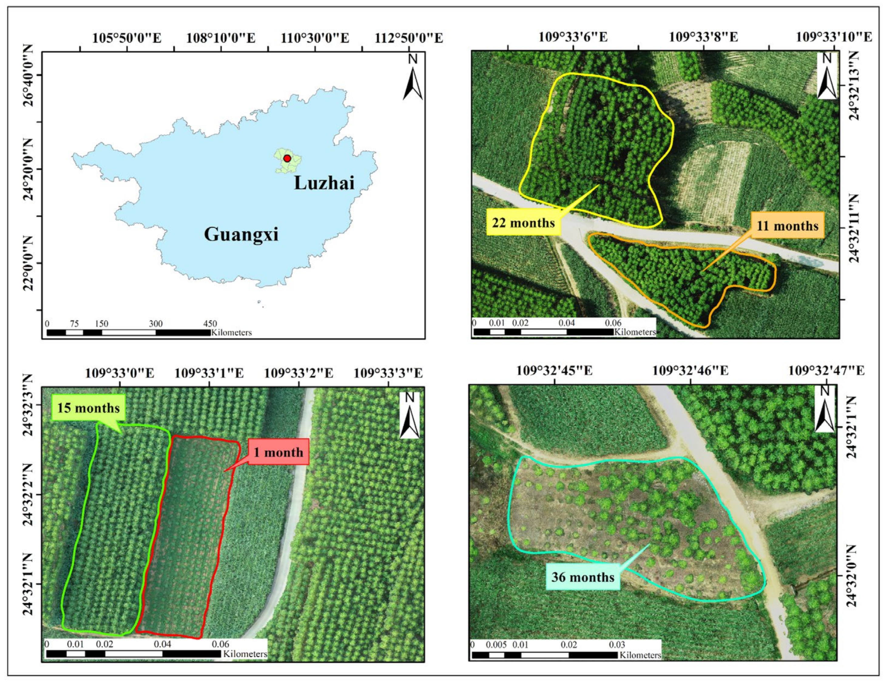
2.1. Study Area

The study area is located in Luzhai County, Liuzhou City, Guangxi Zhuang Autonomous Area, China (108°28′~110°12′ E, 24°14′~24°50′ N), as shown in Figure 1. The terrain of the study area is low and flat, mainly composed of gentle hills, plateaus, and small plains, with an altitude from 99.1 m to 242.6 m. It has a mild subtropical monsoon climate with abundant rainfall and sufficient sunlight. The annual average temperature is around 20 °C, the annual precipitation is about 1500 mm, and the average annual sunshine duration is about 1600 h. The main tree species in the study area include Eucalyptus (Eucalyptus robusta Smith), Masson Pine (Pinus massoniana Lamb.), Chinese Fir (Cunninghamia lanceolata (Lamb.) Hook), and Camphor Tree (Cinnamomum camphora (L.) Presl.).

2.2. Data Introduction

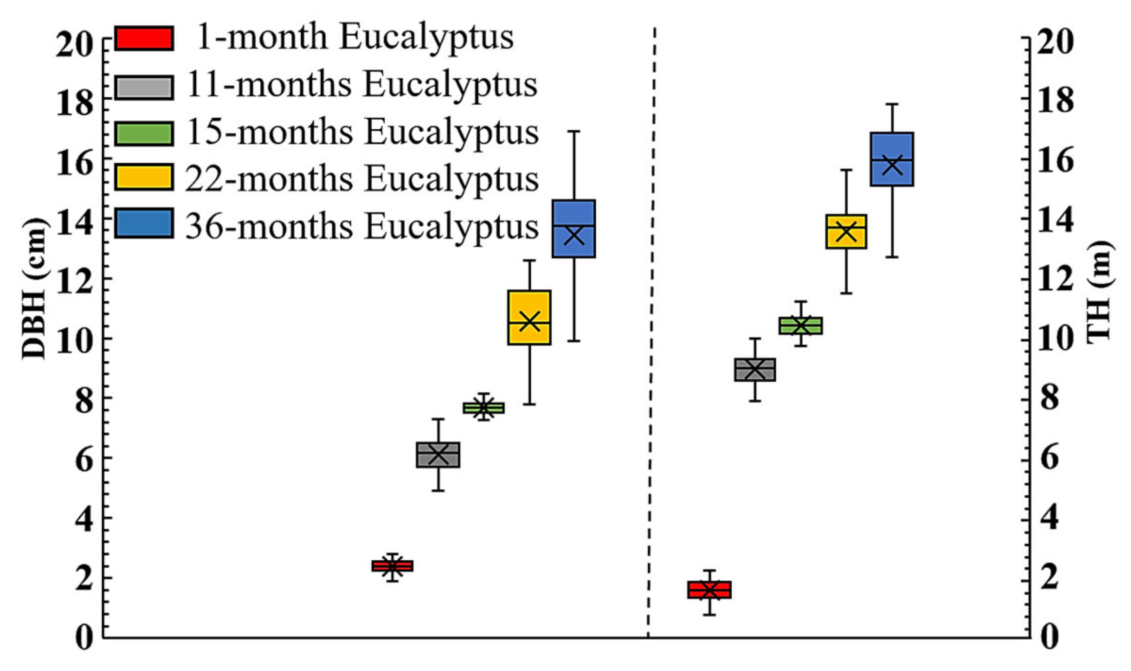
2.2.1. Field Data

Field measurements were conducted in July 2022, and the data obtained mainly included individual tree position, diameter at breast height (DBH), tree height (TH), crown width, and tree age. Among these, the position coordinates of individual trees were obtained using a combination of a total station and a real-time kinematic (RTK). The DBH was obtained using a DBH ruler, and the TH was measured with a Swedish Haglof Vertex Laser ultrasonic altimeter. The distribution of individual tree field measurement data is shown in Figure 2, and the specific statistical results are shown in

Table 1. Statistical results of individual tree field measurement data.

Forest Age (Month)	Number	Average DBH (cm)	DBH SD (cm)	Average TH (m)	TH SD (m)
1	85	2.38	0.21	1.59	0.35
11	52	6.03	0.59	8.93	0.44
15	85	7.68	0.20	10.42	0.33
22	70	10.44	1.16	13.06	0.83
36	57	13.17	1.59	15.84	1.26

Note: diameter at breast height (DBH); tree height (TH); standard definition (SD).

.

2.2.2. UAV Stereo Images

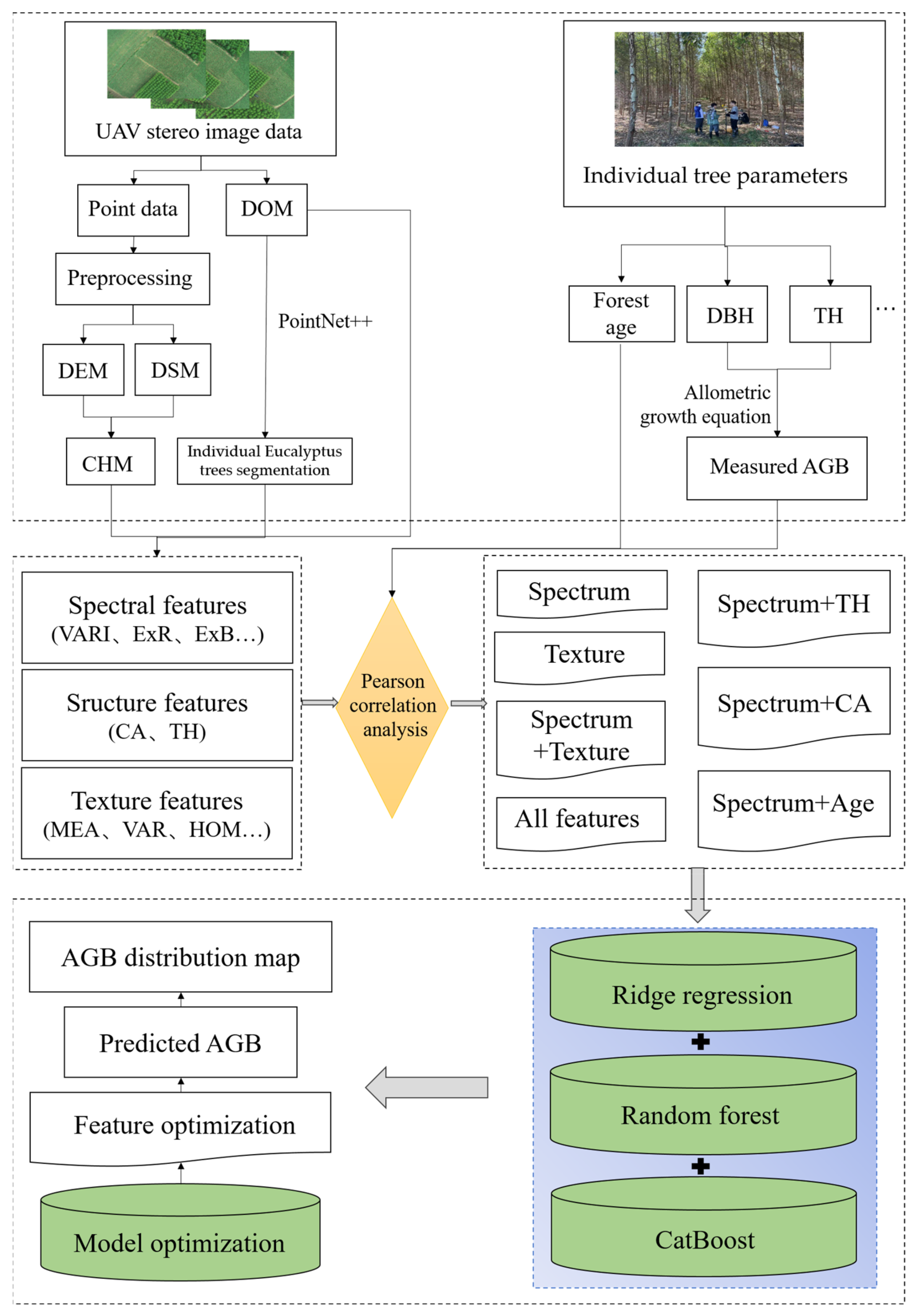
During field data collection, high-resolution stereo images were obtained using a DJI Phantom 4 RTK drone in five-directional flight mode. When collecting images, the weather was clear, with no wind or a light breeze. The flight altitude was 70 m, with an average flight speed of 5.6 m/s. The longitudinal overlap and side overlap were 80% and 70%, respectively. Using the same flight parameters, other stereo images were collected in October 2022 and March 2023 to create AGB spatial distribution maps of individual eucalyptus trees.

2.3. Method

The individual tree AGB was first calculated using the AGB allometric growth equation based on field measurements of individual THs and DBHs. At the same time, the stereo images obtained by the UAV were processed to obtain a digital orthophoto map (DOM) and point data. The point data were denoised and classified, and the elevation was normalized. The classified points were interpolated to generate a digital elevation model (DEM) and a digital surface model (DSM), thereby obtaining a canopy height model (CHM). Meanwhile, the PointNet++ model was used to perform individual tree segmentation based on the normalized point data. Features such as spectrum, texture, TH, and the crown area of individual trees were extracted based on the DOM, CHM, and individual tree segmentation results. Correlation analysis was performed on the extracted features, forest age, and AGB. The features with high correlation were used to construct an AGB model of individual eucalyptus trees using ridge regression, random forest, and the CatBoost algorithm. By comparing the results of models constructed with different algorithms, the optimal model construction algorithm was selected. Then, the features with high correlation were optimized, and the optimal model construction algorithm was used to construct the optimal individual tree AGB estimation model for regional individual eucalyptus tree AGB inversion. Finally, based on the optimal AGB inversion model, the spatial distribution map of individual eucalyptus tree AGB in the study area was obtained. A flowchart of the work is shown in Figure 3.

2.3.1. AGB Calculation of Individual Eucalyptus Trees

Based on field measurements of DBH and TH, the AGB of individual eucalyptus trees was calculated using the eucalyptus allometric growth equation released by the National Forestry Administration in 2014, as shown in Formula (1) [34]:

$$\begin{array}{l}\mathrm{AGB}=0{.02407389(\mathrm{D}}^2{\mathrm{H})}^{0.9768058}+0{.00492556(\mathrm{D}}^2{\mathrm{H})}^{0.8449044}\\ \begin{array}{ccc}& & \end{array}+0{.0007088(\mathrm{D}}^2{\mathrm{H})}^{0.935545}+0{.0063525(\mathrm{D}}^2{\mathrm{H})}^{0.8738162}\end{array}$$

(1)

where AGB represents the aboveground biomass of individual eucalyptus trees (kg/tree), D represents the DBH (cm), and H represents the tree height (m).

The distribution of AGB calculation results for individual eucalyptus trees of different ages is shown in Figure 4.

2.3.2. UAV Stereo Image Processing

The spatial resolution of the images obtained with the UAV was 0.02 m × 0.02 m. The obtained images were processed using the Pix4D V4.7.5 software (Pix4D SA, Prilly, Switzerland) to generate the DSM, DOMs, and point data. The point data were denoised using the Gaussian filtering algorithm, and the denoised point data were classified and manually corrected to obtain ground point data. A DEM was generated with an irregular triangulation interpolation algorithm based on the ground point data. The CHM was obtained by calculating the difference between the DSM and the DEM. Additionally, the denoised point data were normalized based on the DEM to create a segmented dataset for the deep neural network PointNet++. The same procedures were also applied to eucalyptus stereo images from October 2022 and March 2023.

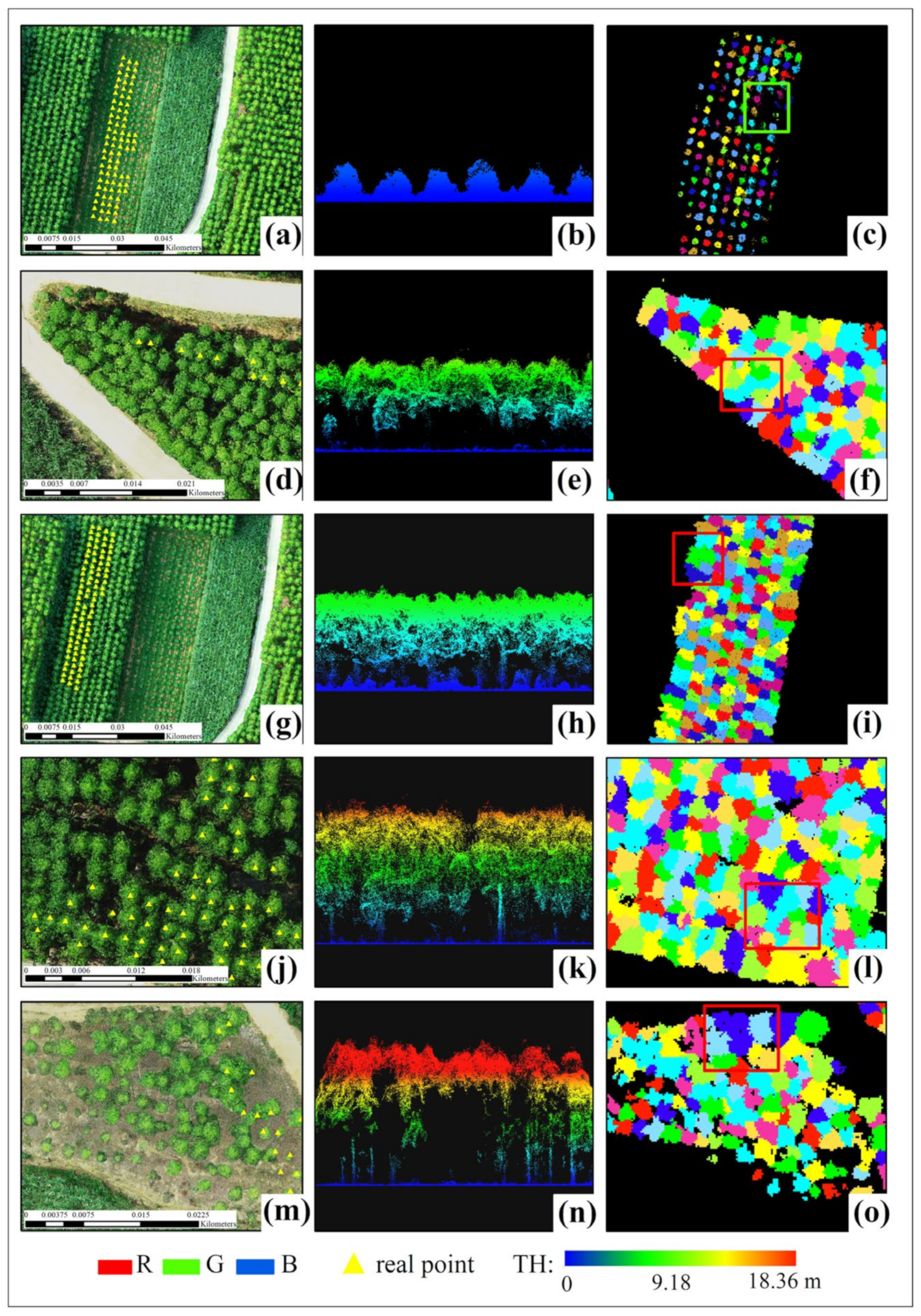
2.3.3. Individual Eucalyptus Tree Segmentation Method

To obtain the spectral reflectance and vegetation index, texture, TH, and crown area features of individual trees, we performed individual tree segmentation on eucalyptus trees. In this study, the classic point cloud segmentation algorithm in deep learning (PointNet++) was used to segment individual eucalyptus trees based on preprocessed point data. The PointNet++ model is an improvement of the PointNet model, which can learn local contextual information and global features [35]. The PointNet model consists of two transformation matrix prediction networks, four multilayer perceptrons (MLPs), and one maximum pooling. The core of the PointNet++ model involves using a set abstraction structure to extract features layer by layer, which includes three parts: sampling, grouping, and PointNet. The specific operating principle is as follows: First, sampling is used to select a certain number of key points, and points within a certain radius area around the key points are used as a grouping. Then, PointNet is performed on the grouping, and finally, the features of each point are obtained. After recognizing tree points in the PointNet++ model, a clustering segmentation algorithm based on point clouds was used to segment the individual tree crowns of the tree points.

Before performing individual tree segmentation, the normalized point data were developed into a training set and a testing set, which included two types of samples: one is individual eucalyptus trees of different ages and growth states, and the other is objects other than eucalyptus trees, including exposed land and other vegetation point data. A total of 345 point samples were produced, including 145 eucalyptus point samples and 200 other samples. Afterward, data augmentation was performed on a limited number of point samples to expand the dataset, including operations such as rotating, randomly shifting, randomly scaling, and randomly discarding, resulting in 2070 point samples. Finally, the expanded point samples were input into the PointNet++ network, and the model was trained and validated at a 7:3 ratio. Meanwhile, key points were selected by setting the farthest point sampling method, and the ball query grouping method was used to divide the grouping. The learning rate was set to 0.001, the batch size was 16, and the number of epochs was 200. Based on the actual growth situation of the five eucalyptus plots, the minimum horizontal spacing between trees was set to 0.3 m.

There were three situations between the reference tree crowns and the segmented tree crowns: true positive (TP), false positive (FP), and false negative (FN). They represent correct segmentation, over-segmentation, and under-segmentation situations. The recall (R), precision (P), and F score (F) were calculated according to Formulas (2)–(4), respectively, to evaluate the segmentation accuracy of individual trees.

$$\mathrm{R}=\frac{\mathrm{TP}}{\mathrm{TP}+\mathrm{FN}}$$

(2)

$$\mathrm{P}=\frac{\mathrm{TP}}{\mathrm{TP}+\mathrm{FP}}$$

(3)

$$\mathrm{F}=2\times \frac{\mathrm{P}\times \mathrm{R}}{\mathrm{P}+\mathrm{R}}$$

(4)

2.3.4. Features Extraction

(1)

Individual Tree Crown Area and TH

Based on the individual tree segmentation results, the areas covered by crown boundaries and crown vertex height information were extracted as the crown area and the THs of individual eucalyptus trees.

(2)

Spectral Reflectance and Vegetation Index

To extract the spectral and vegetation index of the UAV images, the numerical value (DN) of the RGB bands was first normalized using Formulas (5) and (6). Then, the normalized DN value was used to calculate the vegetation index based on the vegetation index calculation formula, as shown in

Table 2. Vegetation index extraction based on UAV orthophoto images.

VI	Name	Formula	Reference
VARI	Visible Atmospherically Resistant Index	(g − r)/(g + r − b)	[36]
ExR	Excess Red Vegetation Index	1.4r − g	[37]
ExB	Excess Blue Vegetation Index	1.4b − g	[38]
ExG	Excess Green Vegetation Index	2g − r − b	[38]
ExGR	Excess Green minus Excess Red Vegetation Index	ExG − ExR	[38]
WI	Woebbecke Index	(g − b)/(r − g)	[39]
IKAW	Kawashima Index	(r − b)/(r + b)	[40]
GLA	Green Leaf Algorithm	(2g – r − b)/(2g + r + b)	[41]
CIVE	Color Index of Vegetation	0.441r − 0.881g + 0.385b + 18.78745	[38]
COM	Combination	0.25ExG + 0.3ExGR + 0.33CIVE + 0.12VEG	[38]
GRRI	Green–Red Ratio Index	G/R	[40]
GBRI	Green–Blue Ratio Index	G/B	[40]
RBRI	Red–Blue Ratio Index	R/B	[40]
INT	Color Intensity Index	(R + G + B)/3	[40]
VEG	Vegetative	g/r0.667 × b0.333	[42]
MGRVI	Modified Green–Red Vegetation Index	(g2 − r2)/(g2 + r2)	[43]

. Based on the previous individual tree crown segmentation results, the vector boundary of the individual tree crowns was overlaid on the normalized RGB image and vegetation index images to mask each tree crown. The mean value of the individual tree crowns was calculated as the spectral reflectance and vegetation index of the individual eucalyptus trees.

$$r=\frac{R}{R+G+B}$$

(5)

$$g=\frac{G}{R+G+B}$$

(6)

$$b=\frac{B}{R+G+B}$$

(7)

(3)

Texture Features

Texture features represent the spatial arrangement attributes of image colors or intensity, which can quantitatively reflect the structure and spatial change information of forest canopies [44]. To extract the texture features of individual eucalyptus trees, based on the segmentation results of the individual tree crowns, the texture features were extracted using the vector boundary of the individual tree crowns as the window size, mainly including mean (MEA), variance (VAR), homogeneity (HOM), contrast (CON), dissimilarity (DIS), entropy (ENT), second-order moment (SEM), and correlation (COR). The specific calculation formulas are shown in

Table 3. Textural feature extraction based on UAV orthophoto images.

Textural Features	Formula
Mean (MEA)	$\mathrm{mean}={\displaystyle \sum _{{}_{i,j}}^{N-1}i{P}_{i,j}}$
Variance (VAR)	$\mathrm{var}={\displaystyle \sum _{{}_{i,j=0}}^{N-1}i{P}_{i,j}{(i-mean)}^2}$
Homogeneity (HOM)	$\mathrm{hom}={\displaystyle \sum _{i,j=0}^{N-1}i\frac{P_{i,j}}{1+{(i-j)}^2}}$
Contrast (CON)	$\mathrm{con}={\displaystyle \sum _{i,j=0}^{N-1}i{P}_{i,j}{(i-j)}^2}$
Dissimilarity (DIS)	$\mathrm{dis}={\displaystyle \sum _{i,j=0}^{N-1}i{P}_{i,j}\left|i-j\right|}$
Entropy (ENT)	$\mathrm{ent}={\displaystyle \sum _{i,j=0}^{N-1}i{P}_{i,j}(-\ln P_{i,j})}$
Second Moment (SEM)	$\mathrm{sm}={\displaystyle \sum _{i,j=0}^{N-1}i{P}_{i,j}^2}$
Correlation (COR)	$\mathrm{corr}={\displaystyle \sum _{i,j=0}^{N-1}i{P}_{i,j}\left[\frac{(i-\mathrm{mean})(j-\mathrm{mean})}{\sqrt{{\mathrm{var}}_i*{\mathrm{var}}_j}}\right]}$

Note: $P_{i,j}=V_{i,j}/{\displaystyle \sum _{i,j=0}^{N-1}{V}_{i,j}}$; V_i,j represents the pixel brightness value at the position of line i and column j, and N represents the size of the moving window when calculating texture features.

.

2.3.5. Feature Combination and Feature Optimization

Based on the feature extraction results, the correlations between the different features and the AGB of individual eucalyptus trees were analyzed in order to select features with higher correlations for different feature combinations. The AGB estimation models were established based on different feature combinations to verify the impact of different features. The SHAP model was used to calculate the importance of each feature variable in the AGB model, thereby constructing a feature optimization AGB estimation model. Based on the concept of Shapley values in cooperative game theory, the SHAP model provides explanations for the contribution of each feature to the prediction results, and it can provide both global and local explanations. In this study, SHAP values were calculated and visualized using “shap” library V0.41.0 in Python.

2.3.6. AGB Estimation Model Construction Algorithms

To explore the impact of different algorithms on the AGB estimation of individual eucalyptus trees, three machine learning algorithms (ridge regression, random forest, and CatBoost) were used to construct AGB models. The details of each algorithm are as follows.

(1)

Ridge regression

Ridge regression is essentially an improved least squares estimation method [45]. By sacrificing the unbiased nature of the least squares method, a more practical and reliable regression method with regression coefficients is obtained at the cost of losing some information and reducing accuracy [46]. In this study, the third-party “Ridge” library of “sklearn” library V1.0.2 in Python was used to construct a ridge regression AGB model. The “alpha” parameter, which controlled the intensity of regularization, was set to 0.005.

(2)

Random forest

Random forest is a powerful machine learning algorithm that combines the prediction results of multiple decision tree models for classification or regression [47]. The decision trees of multiple subsets of data are obtained by bootstrap sampling the training data. At each node of the decision tree, the data subset is randomly divided based on its features to increase the diversity of the model. Ultimately, the prediction results of each decision tree are aggregated through voting or averaging to obtain the final prediction results. Random forest exhibits strong robustness and generalization ability, enabling it to handle high-dimensional data and a large number of features while also demonstrating a certain tolerance for noise and overfitting. In this study, the third-party “RandomForestRegressor” library of “sklearn” library V1.0.2 in Python was used to construct a random forest AGB model. The “n_estimators” parameter was set to 100, and the “random_state” parameter was set to 42.

(3)

CatBoost

CatBoost is a gradient-boosting decision tree algorithm specifically designed for classification and regression tasks [48]. The model uses a decision tree based on the gradient-boosting algorithm as the foundational model, iteratively training multiple weak learners and combining them to form a powerful ensemble model. The unique feature of CatBoost is that it introduces a method of encoding category-based features and addresses the issue of category imbalance by sorting feature statistical information. In this study, “CatBoostRegressor” library V1.1.1 in Python was used to construct a CatBoost AGB model. The “Iterations” parameter specified the number of promotion iterations (set to 1500), the learning rate was the step size of each iteration (set to 0.01), and the depth controlled the depth of the tree in the integration (set to 8).

2.3.7. Accuracy Evaluation

To better evaluate the advantages and disadvantages of AGB models constructed with different features and algorithms, a ten-fold cross-validation was used for model evaluation. The evaluation indicators included the coefficient of determination (R²), the root-mean-square error (RMSE), the normalized RMSE (NRMSE), and Bias. The specific calculation formulas are shown in Formulas (8)–(11):

$$R^2(y,\widehat{y})=1-\frac{{\displaystyle {\sum }_{i=1}^N{(y_i-{\widehat{y}}_i)}^2}}{{\displaystyle {\sum }_{i=1}^N{(y_i-\overline{y})}^2}}$$

(8)

$$\mathrm{RMSE}(y,\widehat{y})=\sqrt{\frac{{\displaystyle {\sum }_{i=1}^N{(y_i-{\widehat{y}}_i)}^2}}{N}}$$

(9)

$$\mathrm{NRMSE}=\frac{\mathrm{RMSE}}{\overline{y}}$$

(10)

$$\mathrm{Bias}(y,\widehat{y})=\frac{{\displaystyle {\sum }_{i=1}^N(y_i-{\widehat{y}}_i)}}{N}$$

(11)

where y represents the measured AGB, ӯ represents the average of the measured AGB, and ŷ represents the estimated AGB. N represents the number of test samples used for evaluation. High R² values were preferred, while lower RMSE, NRMSE, and Bias values indicated better performance by an AGB model.

3. Result and Analysis

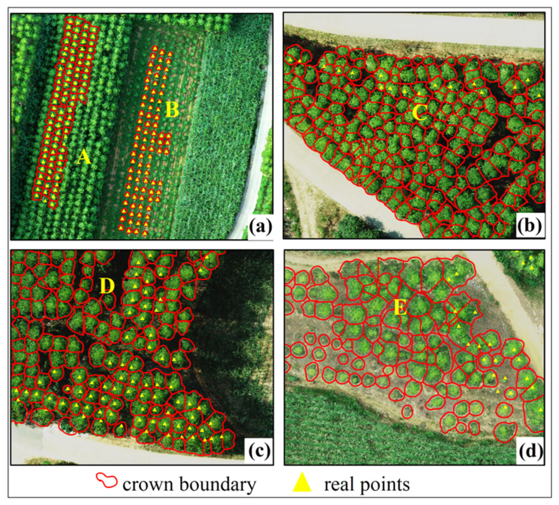
3.1. Individual Tree Segmentation Results for the Eucalyptus Plantations

The segmentation results for individual eucalyptus trees with five different ages using the PointNet++ algorithm are shown in

Table 4. The segmentation results for individual eucalyptus trees with five different ages.

Forest Age (Month)	Number	TP	FN	FP	R	P	F
1	85	85	0	0	1	1	1
11	25	20	2	3	0.91	0.87	0.89
15	91	86	0	5	1	0.95	0.97
22	79	69	0	10	1	0.87	0.93
36	20	16	0	4	1	0.80	0.89

Note: TP, true positive; FN, false negative; FP, false positive; R, recall; P, precision; F, F score.

.

Table 4 shows that the F-scores of the segmentation results of individual eucalyptus trees with five different ages were all greater than 0.89. Of these, the individual tree segmentation accuracy for 1-month-old eucalyptus plantations was the highest, with F being one. The segmentation results for 1-month-old eucalyptus trees were better because of their relatively small crown sizes and larger gaps between trees. These factors contributed to improved individual tree segmentation results. However, the individual tree segmentation accuracy for 11- and 36-month-old eucalyptus plantations was relatively low, with F-scores of 0.89 for each. This was mainly because the 11-month-old sample plots comprised second-generation eucalyptus trees, with two or three individual trees growing on each stump after logging. The spacing between the trees was relatively small, resulting in poor individual tree segmentation results. Although the space between trees in the 36-month-old plot was relatively large, the tree crowns were relatively large, and some adjacent tree crowns were connected, resulting in poor individual segmentation results. The specific segmentation results for individual eucalyptus trees with five different ages are shown in Figure 5.

Figure 5 shows that the PointNet++ algorithm effectively achieved the individual tree segmentation of eucalyptus plantations of different ages. However, there were still incorrect segmentations in certain areas, as shown in the areas marked with green and red boxes in Figure 5.

3.2. Extraction Results for Individual Tree Crown Areas and TH

The above analysis shows that there was some over-segmentation and under-segmentation in the individual tree segmentation results based on the PointNet++ algorithm. To improve the extraction accuracy of the individual tree crown areas, manual adjustments were made to the vector boundaries of the incorrectly segmented individual tree crowns, as shown in Figure 6.

Based on the vector boundaries of individual tree crowns, the crown areas and THs of individual trees were extracted, and a correlation analysis was conducted with the field-measured crown areas and THs of individual trees. The results are shown in Figure 7.

Figure 7 shows that both the extraction accuracies for individual tree crown areas and THs were high, with an R² higher than 0.91. The accuracy of crown area extraction was lower than that of TH extraction. This is mainly because there were certain gaps between the canopies of individual eucalyptus trees, which were not completely connected. However, in most cases, the segmented individual tree canopies were completely connected, which led to some differences between the extracted individual tree crown areas and the measured crown areas.

3.3. Correlation Analysis Results between Features and AGB

Based on feature extraction, the Pearson correlation between 19 spectral features, 24 texture features, TH, crown area, forest age, and AGB was statistically analyzed, and the results are shown in Figure 8.

Figure 8 shows that, among all the features, the correlation between forest age and the AGB of individual eucalyptus trees was the highest, with a correlation coefficient of 0.84, followed by the correlation between TH and AGB, which was 0.80. For texture features, VAR-G had the highest correlation, with a correlation coefficient of −0.69. The correlation coefficient between crown area and AGB was 0.55. The correlation between spectral features and AGB was the lowest, with the spectral reflectance of band b having the highest correlation with AGB at 0.52. Regarding spectral features, feature variables with a correlation greater than 0.5 included b, RBRI, IKAW, and GBRI, while for texture features, variables with a correlation greater than 0.5 included HOM-G, HOM-R, HOM-B, VAR-G, CON-G, and DIS-G. All feature variables with a correlation greater than 0.5 were used for the subsequent AGB modeling of individual eucalyptus trees.

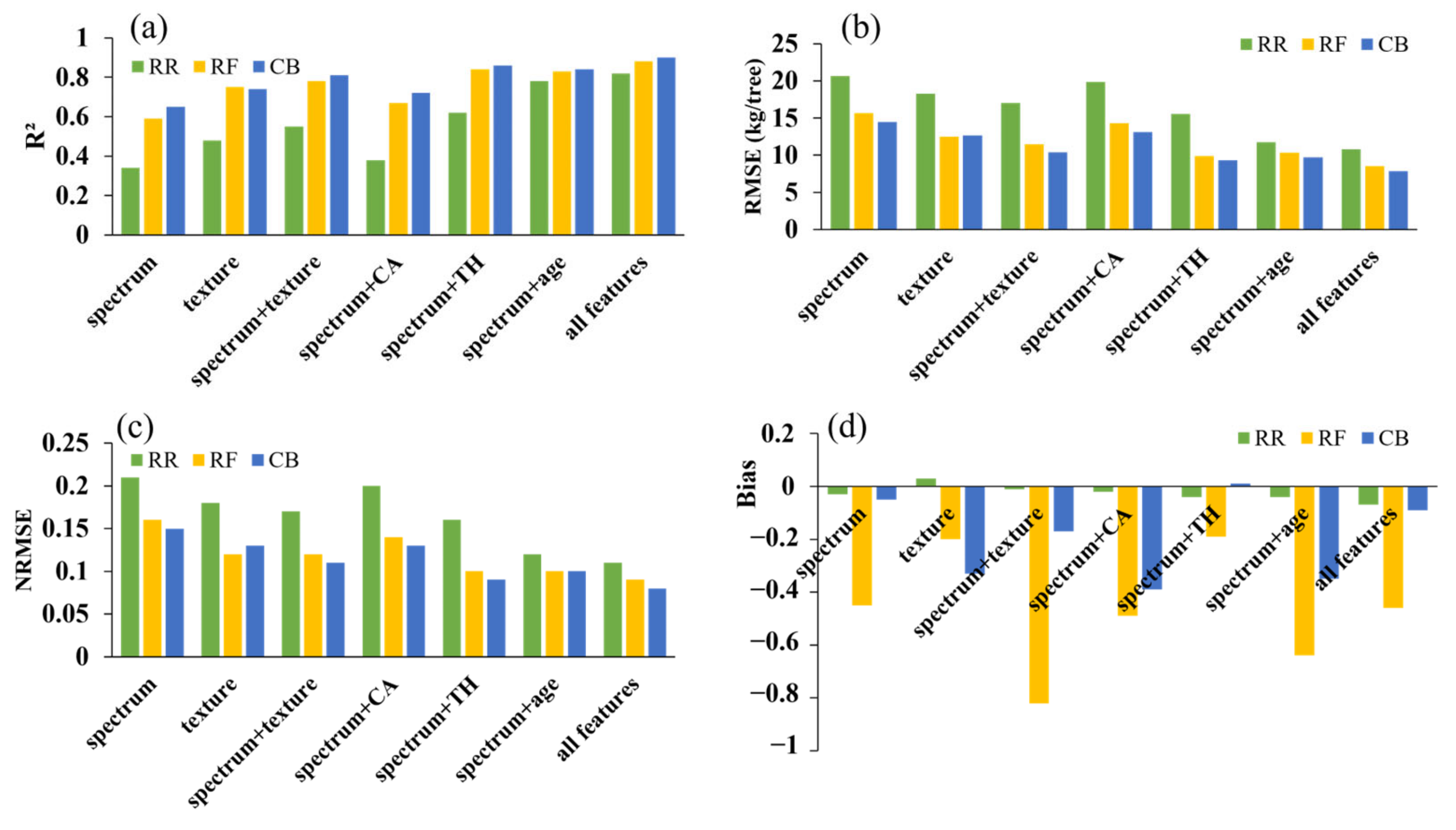
3.4. AGB Estimation Results for Individual Eucalyptus Trees Based on Different Feature Combinations

Based on the above correlation analysis results between the features and AGB, different feature combinations were used to estimate the AGB of individual eucalyptus trees with three algorithms (ridge regression, random forest, and CatBoost), as shown in Figure 9.

Figure 9 shows that, for the AGB estimation results of multiple feature combinations, the model including all features was best. The R² of the ridge regression model was 0.82, the RMSE was 10.79 kg/tree, the NRMSE was 0.11, and the Bias was −0.07. The R² of the CatBoost model was 0.90, the RMSE was 7.85 kg/tree, the NRMSE was 0.08, and the Bias was −0.09. The estimation results of the model with the combination of spectral features and TH followed in terms of accuracy. The R² of the ridge regression model was 0.62, the RMSE was 15.56 kg/tree, the NRMSE was 0.16, and the Bias was −0.04. The R² of the CatBoost model was 0.86, the RMSE was 9.30 kg/tree, the NRMSE was 0.09, and the Bias was 0.01. The estimation results of the model with only spectral features had the lowest accuracy. The R² of the ridge regression model was 0.34, the RMSE was 20.65 kg/tree, the NRMSE was 0.21, and the Bias was −0.03. The R² of the CatBoost model was 0.65, the RMSE was 14.49 kg/tree, the NRMSE was 0.15, and the Bias was −0.05. Compared with the spectral features, the addition of TH, forest age, texture, and crown area improved the estimation accuracy of the model. This showed that a combination of multiple features can improve the estimation accuracy of the individual eucalyptus tree AGB model.

Of the three algorithms, CatBoost had the highest estimation accuracy for all the feature variable combinations, followed by random forest. The difference in the R² values of the estimation results between CatBoost and random forest was not significant, while the result of the ridge regression was the lowest. However, Figure 9d shows that the Bias of the random forest result was much greater than that of the CatBoost result. Therefore, CatBoost was the most suitable algorithm for estimating the AGB of individual eucalyptus trees.

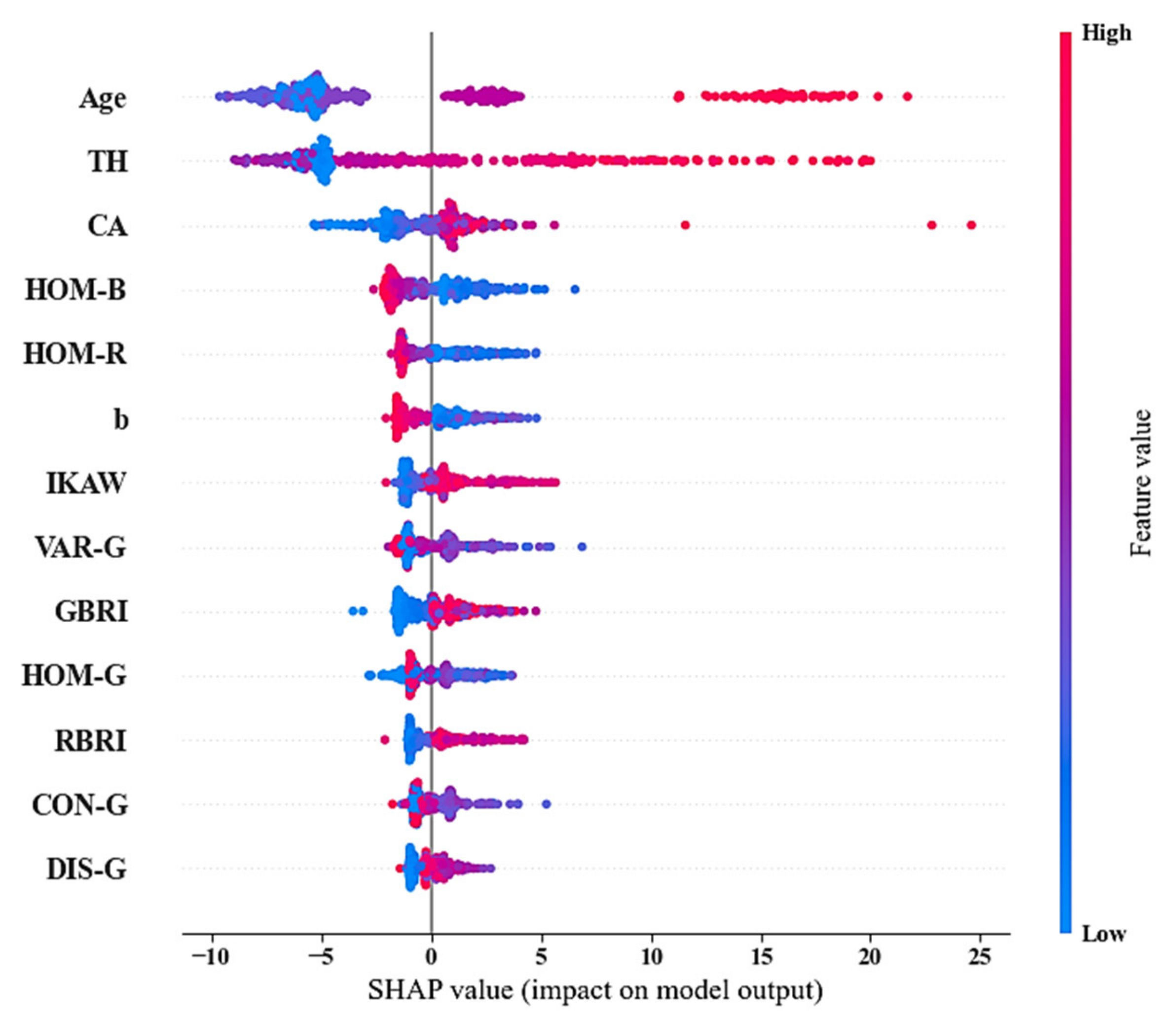
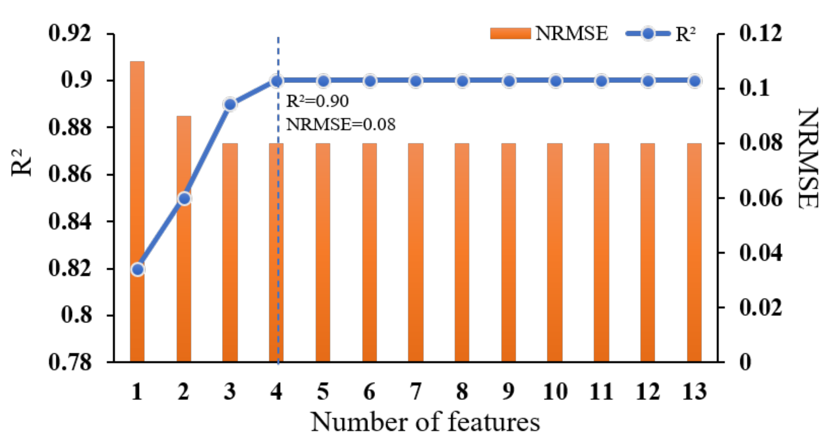
3.5. AGB Estimation Results for Individual Eucalyptus Trees Based on Feature Optimization

Although the combination of multiple feature variables can improve the model’s estimation accuracy, excessive feature variables can not only increase computational costs but also may reduce model accuracy. Therefore, to obtain the optimal AGB estimation model based on the CatBoost algorithm, SHAP (SHapley Additive exPlanations) was used to evaluate the importance of 13 feature variables with a correlation greater than 0.5 with AGB, including spectrum, texture, tree height, crown area, and forest age. The results are shown in Figure 10.

Figure 10 shows that, among the 13 feature variables, forest age was the most important, followed by TH and crown area. In the texture features, HOM-B and HOM-R were relatively important but still lower than TH and crown area. Regarding spectral features, b and IKAW were relatively important but still lower than HOM-B and HOM-R. This result was consistent with the correlation analysis results between features and AGB.

Based on the importance results for the feature variables, the feature variables were sequentially added to the CatBoost model. The AGB estimation results are shown in Figure 11.

Figure 11 shows that, as the number of feature variables increased, the accuracy of the model gradually improved. When the number of feature variables reached four, namely, forest age, tree height, crown area, and HOM-B, the accuracy of the model was highest, with an R² of 0.90 and an NRMSE of 0.08. Afterward, the accuracy of the model did not increase with an increase in feature variables. Therefore, the model constructed with tree height, forest age, crown area, and HOM-B feature variables using the CatBoost algorithm was used to estimate the AGB of individual eucalyptus trees. Correlation analysis was performed with the AGB calculated from the field-measured data, and the results are shown in Figure 12.

Figure 12 shows the correlation analysis results between the estimated AGB and the AGB calculated from field-measured data were good, with an R² of 0.90, an RMSE of 7.93 kg/tree, an NRMSE of 0.08, and a Bias of 0.04. The results indicated that the AGB estimation model constructed based on feature optimization using the CatBoost algorithm can be used to estimate the AGB of individual trees in regional eucalyptus plantations.

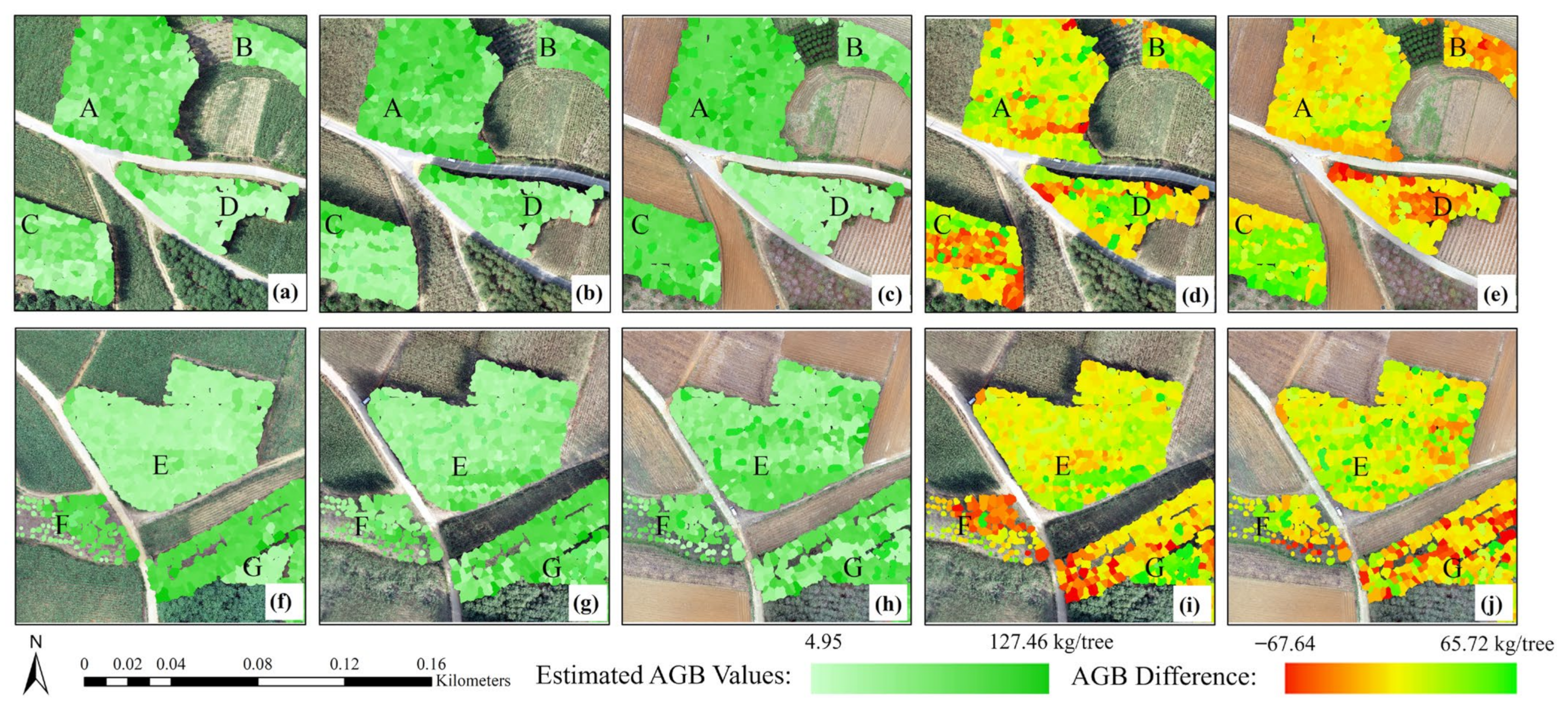
3.6. Spatial Distribution Results for Individual Tree AGB in Eucalyptus Plantations Based on the Optimal Estimation Model

Based on the optimal feature optimization AGB estimation model, the spatial distribution of individual AGB in eucalyptus plantations in July 2022, October 2022, and March 2023 was inverted. The results are shown in Figure 13.

Figure 13 shows that the AGB of individual eucalyptus trees had a gradual growth trend in July 2022, October 2022, and March 2023 but a negative growth trend in some regions. For example, in plot C, negative growth occurred in some regions from July 2022 to October 2022 and from October 2022 to March 2023. There are two main reasons for negative growth: On the one hand, given the influence of wind and rain, some eucalyptus trees collapsed, resulting in significant changes in the tree height extraction, leading to negative growth. On the other hand, given that some eucalyptus plots are natural regeneration plots of the second or third generation, such as plot D, each logging stump usually retains two to three eucalyptus trees first. During the eucalyptus trees growth process, they will be nurtured and felled to retain one or two well-growing trees, which will also lead to negative AGB growth.

4. Discussion

4.1. Analysis of Different Feature Variables in Eucalyptus AGB Estimation

To explore the impact of different feature variables on the construction of AGB models, spectral features, texture, tree height, and crown area were extracted from UAV stereo images, supplemented by forest age, to explore the impact of different feature variables on estimating individual eucalyptus AGB. Tree height and forest age had the greatest impact on the AGB model, followed by crown area, texture, and spectral features. The results indicated that different feature variables have different impacts on estimating the AGB of individual eucalyptus trees. This is mainly because tree height is a structural parameter closely related to the growth status of trees, which can directly characterize changes in tree AGB. The higher the tree height, the greater the biomass. Meanwhile, the true value of AGB can also be obtained based on field-measured tree heights and DBHs using the biomass allometric growth equation; thus, tree height has the greatest impact on the AGB model. There is also a strong relationship between forest age and AGB, and the older the forest age, the greater the AGB. For fast-growing eucalyptus plantations, the correlation between forest age and AGB is stronger, as shown in Figure 8. The Pearson correlation coefficient between forest age and individual eucalyptus AGB is 0.84. When the SHAP model was used to explain the importance of the 13 features used in the CatBoost algorithm for estimating eucalyptus AGB, forest age also showed significant importance, as shown in Figure 10. As a feature variable that directly characterizes forest tree characteristics, the impact of crown area on the AGB model is relatively low. This is mainly because the spaces between rows and columns in eucalyptus plantations are relatively fixed, mostly about 2 m × 3 m. Under this planting situation, the crown area of eucalyptus trees does not change significantly at different growth stages of forest age, so the correlation between crown area and AGB is weaker than that of tree height and forest age. Although texture and spectral features have an impact on AGB, it is lower than that of tree height, forest age, and crown area. This is mainly because the texture and spectral features are not directly related to the AGB of individual eucalyptus trees but indirectly represent the AGB by characterizing the individual crowns of eucalyptus trees. Therefore, the impact of texture and spectral features is weaker than those of AGB that directly characterize feature variables such as tree height, forest age, and crown area. Similar conclusions were drawn in previous studies. For example, Gao et al. [49] extracted spectral, vegetation index, texture, and other features from hyperspectral data and extracted tree height, canopy structure, and other information from airborne LiDAR data. The features were screened and combined to estimate the AGB of different tree species in artificial forests. The results indicated that eucalyptus AGB has the best correlation with features extracted from LiDAR data. Zhao et al. [50] extracted the texture, spectrum, and crown area features of forest shrubs from multispectral images and extracted the height and volume features of each shrub from UAV LiDAR data. The features were screened and combined to estimate shrub AGB. The results indicated that structural features were the most important predictive factors for predicting individual shrub AGB values, while texture and spectrum exhibited a relatively weak performance. Dos Reis et al. [51] used random forest algorithms to estimate the volume of eucalyptus plantations based on Landsat 8 images, Sentinel-1B, terrain data, and forest age based on forest inventory data. The results showed that the volume estimation based on forest age was the best of out all the single data sources, with an R² of 0.49. Zheng et al. [52] explored the effects of vegetation index, leaf area index, and forest age on the estimation of AGB in different forest types via stepwise regression analysis based on remote sensing data. The results showed that forest age is an important variable in estimating AGB. Once the forest age exceeds a certain threshold, the leaf area remains almost unchanged, while the forest biomass continues to accumulate. Therefore, in the future, time series satellite image data such as high-resolution series images can be used to extract the spatial distribution of eucalyptus plantation ages, and tree heights extracted from ICESat-2 photon cloud data can be combined to invert the spatial distribution of eucalyptus plantation biomass in large regions.

4.2. Analysis of Different Algorithms on Eucalyptus AGB Estimation

In addition to feature variables, the model’s construction algorithm is also a key factor affecting the accuracy of biomass estimation. To explore the impact of different algorithms on estimating the AGB of individual eucalyptus trees, three machine learning algorithms, namely, ridge regression, random forest, and CatBoost, were used to estimate the AGB of individual eucalyptus trees based on different feature variables. The results indicated that the CatBoost algorithm has the best estimation accuracy, followed by the random forest algorithm, and the ridge regression algorithm has the lowest estimation accuracy. This is mainly related to the characteristics of the algorithm itself. For example, the CatBoost algorithm has a built-in mechanism for handling overfitting, gradually and effectively optimizing the model through gradient enhancement strategies, and it has a good generalization ability, making it suitable for processing large-scale datasets. Compared with the CatBoost algorithm, the random forest algorithm performs relatively weakly, mainly because it requires additional processing when dealing with imbalanced data, such as using weights or data sampling methods, while the CatBoost algorithm has strong robustness. Meanwhile, when processing data with fewer samples or high-dimensional features, the random forest algorithm may experience overfitting or performance degradation; the CatBoost algorithm is more robust in this situation. The ridge regression algorithm is a linear model that is more suitable for data with linear relationships between features. Although introducing a regularization term can prevent overfitting in the model, when the data are complex or the relationship between features and targets is complex, ridge regression may not be sufficient to capture these complex relationships, resulting in underfitting. In addition, the ridge regression algorithm may include features that have redundancy or no impact on the results when processing features. This is consistent with previous research findings. For example, Zhang et al. [33] used eight methods to estimate forest AGB based on multi-satellite data products. The results showed that five tree-based ensemble algorithms performed better than three nonensemble algorithms (multivariate adaptive regression splines, support vector regression, and multilayer perceptron). Ye et al. [53] estimated AGB for black local-planted forests based on machine learning regression methods (support vector machine, artificial neural network, and random forest). The results indicated that the AGB estimation model based on random forest was optimal, with a maximum R² of 0.85. Although machine learning algorithms can estimate the AGB of individual eucalyptus trees, compared with deep learning algorithms, machine learning algorithms still have some shortcomings in mining data information. Deep learning algorithms can automatically learn higher-level feature representations from raw data, which helps to mine deeper information and achieve higher accuracy estimation in AGB models. Therefore, to further explore the deep-level information between UAV multi-feature variables and AGB, deep learning algorithms such as convolutional neural networks (CNNs) or recurrent neural networks (RNNs) should be considered in the future to estimate AGB in eucalyptus plantations.

5. Conclusions

We used UAVs to obtain stereo images, and different algorithms were used to study the impact of UAV-derived features and forest ages on estimates of the AGB of individual eucalyptus trees. The main conclusions are as follows:

(1)

The impact of different features on estimating the AGB of individual eucalyptus trees varies, with TH having the greatest impact, followed by forest age, with texture, crown area, spectral reflectance, and vegetation index having relatively small effects.

(2)

Of the three algorithms, the model established with CatBoost had the highest accuracy, with an R² ranging from 0.65 to 0.90, an NRMSE ranging from 0.08 to 0.15, and a Bias ranging from −0.39 to 0.01, followed by the random forest algorithm, with an R² ranging from 0.59 to 0.88, an NRMSE ranging from 0.09 to 0.16, and a Bias ranging from −0.82 to −0.19. The ridge regression algorithm had the lowest accuracy, with an R² ranging from 0.34 to 0.82, an NRMSE ranging from 0.11 to 0.21, and a Bias ranging from −0.07 to 0.03.

(3)

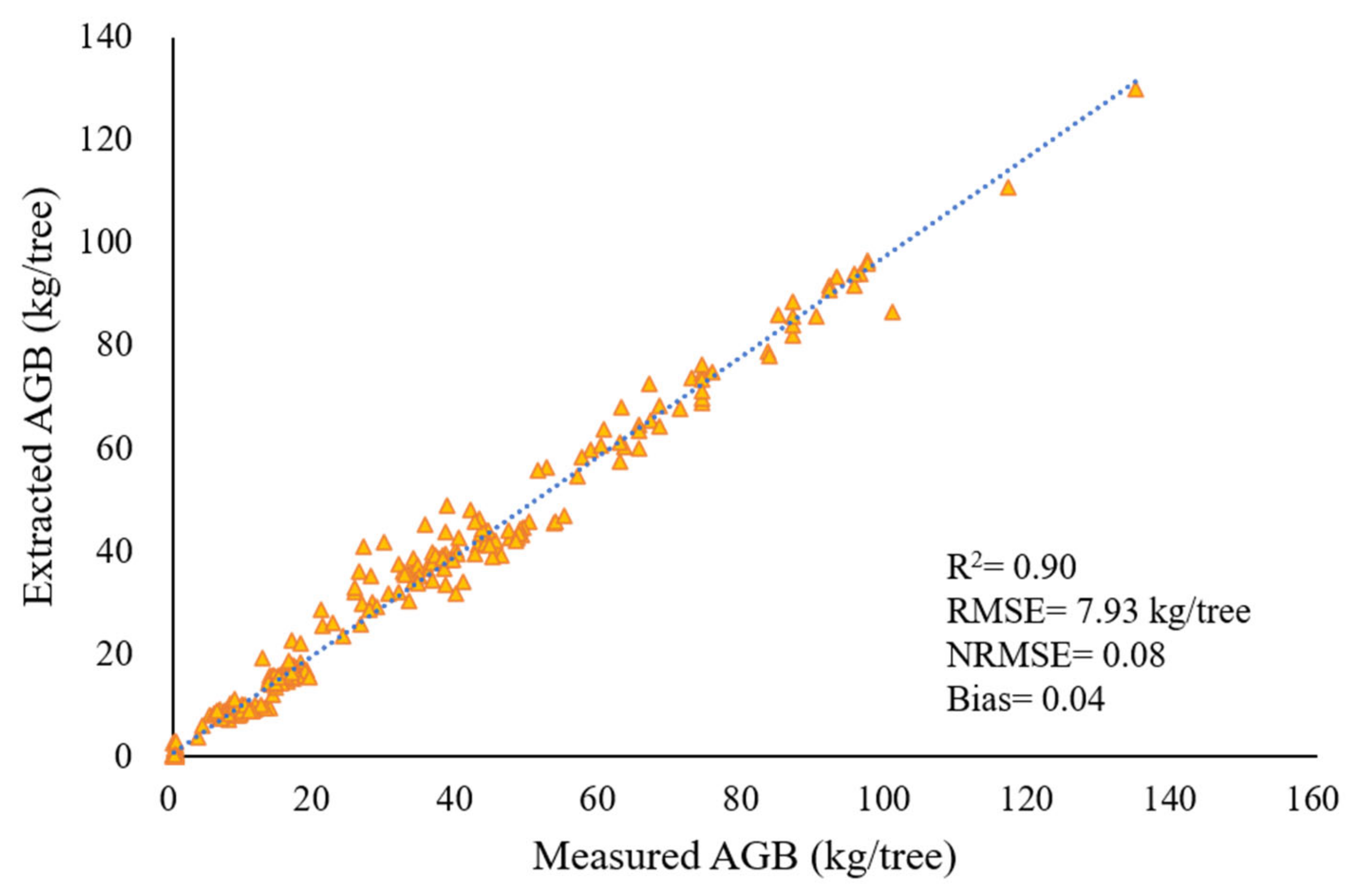
Accurately estimating the AGB of individual eucalyptus trees can be achieved based on UAV stereo images. The model constructed with TH, forest age, crown area, and HOM-B feature variables using the CatBoost algorithm had the best estimation accuracy, with an R² of 0.90 and an NRMSE of 0.08.

The potential of using UAV stereo image data to estimate the AGB of individual eucalyptus trees was explored in this study, and the results can provide methodological references and technical support for subsequent estimation studies of forest biomass, carbon storage, and other structural parameters requiring UAV data. However, given the relatively flat terrain of the sample plots we used, the small forest age range, and the fact that all three algorithms were machine learning algorithms, the practicality of the results in more complex situations needs further verification. Therefore, we plan to select eucalyptus plantation plots with more complex terrain and larger tree age ranges in future research and use deep learning algorithms to further explore the application potential of estimating eucalyptus AGB based on UAV stereo images, thus providing high-precision basic data for eucalyptus plantation planning, management, and policy formulation.

References

1. Schönau, A. Silvicultural considerations for high productivity of Eucalyptus grandis. For. Ecol. Manag. 1984, 9, 295–314. [Google Scholar] [CrossRef]
2. Silverio, F.O.; Barbosa, L.C.A.; Maltha, C.R.A.; Silvestre, A.J.D.; Pilo-Veloso, D.; Gomide, J.L. Characterization of lipophilic wood extractives from clones of Eucalyptus urograndis cultivate in Brazil. BioResources 2007, 2, 157–168. [Google Scholar] [CrossRef]
3. González-García, M.; Hevia, A.; Majada, J.; De Anta, R.C.; Barrio-Anta, M. Dynamic growth and yield model including environmental factors for Eucalyptus nitens (Deane & Maiden) Maiden short rotation woody crops in Northwest Spain. New For. 2015, 46, 387–407. [Google Scholar] [CrossRef]
4. Boisvenue, C.; Smiley, B.P.; White, J.C.; Kurz, W.A.; Wulder, M.A. Integration of Landsat time series and field plots for forest productivity estimates in decision support models. For. Ecol. Manag. 2016, 376, 284–297. [Google Scholar] [CrossRef]
5. Nevalainen, O.; Honkavaara, E.; Tuominen, S.; Viljanen, N.; Hakala, T.; Yu, X.; Hyyppä, J.; Saari, H.; Pölönen, I.; Imai, N.N.; et al. Individual Tree Detection and Classification with UAV-Based Photogrammetric Point Clouds and Hyperspectral Imaging. Remote Sens. 2017, 9, 185. [Google Scholar] [CrossRef]
6. Kumbula, S.T.; Mafongoya, P.; Peerbhay, K.Y.; Lottering, R.T.; Ismail, R. Using Sentinel-2 Multispectral Images to Map the Occurrence of the Cossid Moth (Coryphodema tristis) in Eucalyptus Nitens Plantations of Mpumalanga, South Africa. Remote Sens. 2019, 11, 278. [Google Scholar] [CrossRef]
7. Verma, N.K.; Lamb, D.W.; Sinha, P. Airborne LiDAR and high resolution multispectral data integration in Eucalyptus tree species mapping in an Australian farmscape. Geocarto Int. 2022, 37, 70–90. [Google Scholar] [CrossRef]
8. Berra, E.F.; Brandelero, C.; Pereira, R.S.; Sebem, E.; Goergen, L.C.d.G.; Benedetti, A.C.P.; Lippert, D.B. Total wood volume estimation of Eucalyptus species by images of landsat satellite. Ciênc. Florest. 2012, 22, 853–864. [Google Scholar] [CrossRef]
9. Gebreslasie, M.; Ahmed, F.; Van Aardt, J.A. Extracting structural attributes from IKONOS imagery for Eucalyptus plantation forests in KwaZulu-Natal, South Africa, using image texture analysis and artificial neural networks. Int. J. Remote Sens. 2011, 32, 7677–7701. [Google Scholar] [CrossRef]
10. Johansen, K.; Raharjo, T.; McCabe, M.F. Using Multi-Spectral UAV Imagery to Extract Tree Crop Structural Properties and Assess Pruning Effects. Remote Sens. 2018, 10, 854. [Google Scholar] [CrossRef]
11. Yang, K.; Zhang, H.; Wang, F.; Lai, R. Extraction of Broad-Leaved Tree Crown Based on UAV Visible Images and OBIA-RF Model: A Case Study for Chinese Olive Trees. Remote Sens. 2022, 14, 2469. [Google Scholar] [CrossRef]
12. Latifah, S.; Teodoro, R.; Myrna, G.; Nathaniel, C.; Leonardo, M. Predicted Stand Volume for Eucalyptus Plantations by Spatial Analysis. In IOP Conference Series: Earth and Environmental Science; IOP Publishing: Bristol, UK, 2018; p. 012117. [Google Scholar]
13. Tompalski, P.; Coops, N.C.; Marshall, P.L.; White, J.C.; Wulder, M.A.; Bailey, T. Combining multi-date airborne laser scanning and digital aerial photogrammetric data for forest growth and yield modelling. Remote Sens. 2018, 10, 347. [Google Scholar] [CrossRef]
14. De Moura, Y.M.; Balzter, H.; Galvão, L.S.; Dalagnol, R.; Espírito-Santo, F.; Santos, E.G.; Garcia, M.; Bispo, P.d.C.; Oliveira, R.C.; Shimabukuro, Y.E. Carbon Dynamics in a Human-Modified Tropical Forest: A Case Study Using Multi-Temporal LiDAR Data. Remote Sens. 2020, 12, 430. [Google Scholar] [CrossRef]
15. You, H.; Liu, Y.; Lei, P.; Qin, Z.; You, Q. Segmentation of individual mangrove trees using UAV-based LiDAR data. Ecol. Informatics 2023, 77, 102200. [Google Scholar] [CrossRef]
16. Chan, E.P.Y.; Fung, T.; Wong, F.K.K. Estimating above-ground biomass of subtropical forest using airborne LiDAR in Hong Kong. Sci. Rep. 2021, 11, 1751. [Google Scholar] [CrossRef] [PubMed]
17. Fatoyinbo, T.; Feliciano, E.A.; Lagomasino, D.; Lee, S.K.; Trettin, C. Estimating mangrove aboveground biomass from airborne LiDAR data: A case study from the Zambezi River delta. Environ. Res. Lett. 2018, 13, 025012. [Google Scholar] [CrossRef]
18. Jaakkola, A.; Hyyppä, J.; Yu, X.; Kukko, A.; Kaartinen, H.; Liang, X.; Hyyppä, H.; Wang, Y. Autonomous Collection of Forest Field Reference—The Outlook and a First Step with UAV Laser Scanning. Remote Sens. 2017, 9, 785. [Google Scholar] [CrossRef]
19. Fan, Y.; Feng, H.; Jin, X.; Yue, J.; Liu, Y.; Li, Z.; Feng, Z.; Song, X.; Yang, G. Estimation of the nitrogen content of potato plants based on morphological parameters and visible light vegetation indices. Front. Plant Sci. 2022, 13, 1012070. [Google Scholar] [CrossRef]
20. Tang, X.; You, H.; Liu, Y.; You, Q.; Chen, J. Monitoring of Monthly Height Growth of Individual Trees in a Subtropical Mixed Plantation Using UAV Data. Remote Sens. 2023, 15, 326. [Google Scholar] [CrossRef]
21. Chen, J.; Chen, Z.; Huang, R.; You, H.; Han, X.; Yue, T.; Zhou, G. The Effects of Spatial Resolution and Resampling on the Classification Accuracy of Wetland Vegetation Species and Ground Objects: A Study Based on High Spatial Resolution UAV Images. Drones 2023, 7, 61. [Google Scholar] [CrossRef]
22. Iglhaut, J.; Cabo, C.; Puliti, S.; Piermattei, L.; O’Connor, J.; Rosette, J. Structure from Motion Photogrammetry in Forestry: A Review. Curr. For. Rep. 2019, 5, 155–168. [Google Scholar] [CrossRef]
23. Zarco-Tejada, P.J.; Diaz-Varela, R.; Angileri, V.; Loudjani, P. Tree height quantification using very high resolution imagery acquired from an unmanned aerial vehicle (UAV) and automatic 3D photo-reconstruction methods. Eur. J. Agron. 2014, 55, 89–99. [Google Scholar] [CrossRef]
24. Navarro, J.A.; Algeet, N.; Fernández-Landa, A.; Esteban, J.; Rodríguez-Noriega, P.; Guillén-Climent, M.L. Integration of UAV, Sentinel-1, and Sentinel-2 Data for Mangrove Plantation Aboveground Biomass Monitoring in Senegal. Remote Sens. 2019, 11, 77. [Google Scholar] [CrossRef]
25. You, H.; Tang, X.; You, Q.; Liu, Y.; Chen, J.; Wang, F. Study on the Differences between the Extraction Results of the Structural Parameters of Individual Trees for Different Tree Species Based on UAV LiDAR and High-Resolution RGB Images. Drones 2023, 7, 317. [Google Scholar] [CrossRef]
26. Alonzo, M.; Dial, R.J.; Schulz, B.K.; Andersen, H.-E.; Lewis-Clark, E.; Cook, B.D.; Morton, D.C. Mapping tall shrub biomass in Alaska at landscape scale using structure-from-motion photogrammetry and lidar. Remote Sens. Environ. 2020, 245, 111841. [Google Scholar] [CrossRef]
27. Guerra-Hernández, J.; Cosenza, D.N.; Rodriguez, L.C.E.; Silva, M.; Tomé, M.; Díaz-Varela, R.A.; González-Ferreiro, E. Comparison of ALS-and UAV (SfM)-derived high-density point clouds for individual tree detection in Eucalyptus plantations. Int. J. Remote Sens. 2018, 39, 5211–5235. [Google Scholar] [CrossRef]
28. Guerra-Hernández, J.; Cosenza, D.N.; Cardil, A.; Silva, C.A.; Botequim, B.; Soares, P.; Silva, M.; González-Ferreiro, E.; Díaz-Varela, R.A. Predicting Growing Stock Volume of Eucalyptus Plantations Using 3-D Point Clouds Derived from UAV Imagery and ALS Data. Forests 2019, 10, 905. [Google Scholar] [CrossRef]
29. Dang, A.T.N.; Nandy, S.; Srinet, R.; Luong, N.V.; Ghosh, S.; Kumar, A.S. Forest aboveground biomass estimation using machine learning regression algorithm in Yok Don National Park, Vietnam. Ecol. Inform. 2019, 50, 24–32. [Google Scholar] [CrossRef]
30. Montesano, P.; Cook, B.; Sun, G.; Simard, M.; Nelson, R.; Ranson, K.; Zhang, Z.; Luthcke, S. Achieving accuracy requirements for forest biomass mapping: A spaceborne data fusion method for estimating forest biomass and LiDAR sampling error. Remote Sens. Environ. 2013, 130, 153–170. [Google Scholar] [CrossRef]
31. Gomez, C.; Mangeas, M.; Petit, M.; Corbane, C.; Hamon, P.; Hamon, S.; De Kochko, A.; Le Pierres, D.; Poncet, V.; Despinoy, M. Use of high-resolution satellite imagery in an integrated model to predict the distribution of shade coffee tree hybrid zones. Remote Sens. Environ. 2010, 114, 2731–2744. [Google Scholar] [CrossRef]
32. Selvaraj, M.G.; Vergara, A.; Montenegro, F.; Ruiz, H.A.; Safari, N.; Raymaekers, D.; Ocimatie, W.; Ntamwirac, J.; Titsd, L.; Blomme, G.; et al. Detection of banana plants and their major diseases through aerial images and machine learning methods: A case study in DR Congo and Republic of Benin. ISPRS J. Photogramm. Remote Sens. 2020, 169, 110–124. [Google Scholar] [CrossRef]
33. Zhang, Y.; Ma, J.; Liang, S.; Li, X.; Li, M. An Evaluation of Eight Machine Learning Regression Algorithms for Forest Aboveground Biomass Estimation from Multiple Satellite Data Products. Remote Sens. 2020, 12, 4015. [Google Scholar] [CrossRef]
34. LY/T 2253-2014; Guidelines for Carbon Sink Measurement and Monitoring for Afforestation Projects. SAMR: Beijing, China, 2014.
35. Qi, C.R.; Yi, L.; Su, H.; Guibas, L.J. Pointnet++: Deep Hierarchical Feature Learning on Point Sets in a Metric Space. In Advances in Neural Information Processing Systems; MIT Press: Cambridge, MA, USA, 2017; Volume 30. [Google Scholar]
36. Gitelson, A.A.; Kaufman, Y.J.; Stark, R.; Rundquist, D. Novel algorithms for remote estimation of vegetation fraction. Remote Sens. Environ. 2002, 80, 76–87. [Google Scholar] [CrossRef]
37. Meyer, G.E.; Neto, J.C. Verification of color vegetation indices for automated crop imaging applications. Comput. Electron. Agric. 2008, 63, 282–293. [Google Scholar] [CrossRef]
38. Guijarro, M.; Pajares, G.; Riomoros, I.; Herrera, P.; Burgos-Artizzu, X.; Ribeiro, A. Automatic segmentation of relevant textures in agricultural images. Comput. Electron. Agric. 2011, 75, 75–83. [Google Scholar] [CrossRef]
39. Woebbecke, D.M.; Meyer, G.E.; Von Bargen, K.; Mortensen, D.A. Color Indices for Weed Identification Under Various Soil, Residue, and Lighting Conditions. Trans. ASAE 1995, 38, 259–269. [Google Scholar] [CrossRef]
40. Kawashima, S.; Nakatani, M. An Algorithm for Estimating Chlorophyll Content in Leaves Using a Video Camera. Ann. Bot. 1998, 81, 49–54. [Google Scholar] [CrossRef]
41. Louhaichi, M.; Borman, M.M.; Johnson, D.E. Spatially Located Platform and Aerial Photography for Documentation of Grazing Impacts on Wheat. Geocarto Int. 2001, 16, 65–70. [Google Scholar] [CrossRef]
42. Hague, T.; Tillett, N.D.; Wheeler, H. Automated Crop and Weed Monitoring in Widely Spaced Cereals. Precis. Agric. 2006, 7, 21–32. [Google Scholar] [CrossRef]
43. Bendig, J.; Yu, K.; Aasen, H.; Bolten, A.; Bennertz, S.; Broscheit, J.; Gnyp, M.L.; Bareth, G. Combining UAV-based plant height from crop surface models, visible, and near infrared vegetation indices for biomass monitoring in barley. Int. J. Appl. Earth Obs. Geoinf. 2015, 39, 79–87. [Google Scholar] [CrossRef]
44. Liang, Y.; Kou, W.; Lai, H.; Wang, J.; Wang, Q.; Xu, W.; Wang, H.; Lu, N. Improved estimation of aboveground biomass in rubber plantations by fusing spectral and textural information from UAV-based RGB imagery. Ecol. Indic. 2022, 142, 109286. [Google Scholar] [CrossRef]
45. Hoerl, A.E.; Kennard, R.W. Ridge regression: Biased estimation for nonorthogonal problems. Technometrics 1970, 12, 55–67. [Google Scholar] [CrossRef]
46. Shih, S.F.; Gervin, J.C. Ridge Regression Techniques Applied to Landsat Investigation of Water Quality in Lake Okeechobee. JAWRA J. Am. Water Resour. Assoc. 1980, 16, 790–796. [Google Scholar] [CrossRef]
47. Breiman, L. Random forests. Mach. Learn. 2001, 45, 5–32. [Google Scholar] [CrossRef]
48. Prokhorenkova, L.; Gusev, G.; Vorobev, A.; Dorogush, A.V.; Gulin, A. CatBoost: Unbiased Boosting with Categorical Features. In Advances in Neural Information Processing Systems; MIT Press: Cambridge, MA, USA, 2018; Volume 31. [Google Scholar]
49. Gao, L.; Chai, G.; Zhang, X. Above-Ground Biomass Estimation of Plantation with Different Tree Species Using Airborne LiDAR and Hyperspectral Data. Remote Sens. 2022, 14, 2568. [Google Scholar] [CrossRef]
50. Zhao, Y.; Liu, X.; Wang, Y.; Zheng, Z.; Zheng, S.; Zhao, D.; Bai, Y. UAV-based individual shrub aboveground biomass estimation calibrated against terrestrial LiDAR in a shrub-encroached grassland. Int. J. Appl. Earth Obs. Geoinf. 2021, 101, 102358. [Google Scholar] [CrossRef]
51. Dos Reis, A.A.; Franklin, S.E.; de Mello, J.M.; Junior, F.W.A. Volume estimation in a Eucalyptus plantation using multi-source remote sensing and digital terrain data: A case study in Minas Gerais State, Brazil. Int. J. Remote Sens. 2019, 40, 2683–2702. [Google Scholar] [CrossRef]
52. Zheng, G.; Chen, J.; Tian, Q.; Ju, W.; Xia, X. Combining remote sensing imagery and forest age inventory for biomass mapping. J. Environ. Manag. 2007, 85, 616–623. [Google Scholar] [CrossRef]
53. Ye, Q.; Yu, S.; Liu, J.; Zhao, Q.; Zhao, Z. Aboveground biomass estimation of black locust planted forests with aspect variable using machine learning regression algorithms. Ecol. Indic. 2021, 129, 107948. [Google Scholar] [CrossRef]
Figure 1. Location of the study area.
Forests 14 01748 g001
Figure 2. The distribution of individual tree field measurement data.
Forests 14 01748 g002
Figure 3. Flowchart of the work. Note: tree height, TH; crown area, CA; aboveground biomass, AGB.
Forests 14 01748 g003
Figure 4. Distribution of AGB calculation results for individual eucalyptus trees of different ages.
Forests 14 01748 g004
Figure 5. Individual tree segmentation results for eucalyptus plots with five forest ages. Results for 1-month-old (ac), 11-month-old (df), 15-month-old (gi), 22-month-old (jl), and 36-month-old (mo) eucalyptus with orthophoto mosaic point data derived from stereo images and individual tree segmentation based on point data, from left to right. The green and red boxes in the third column represent incorrect segmentations.
Forests 14 01748 g005
Figure 6. Manual correction results for the individual tree segmentation vector boundary. (a) represents eucalyptus plots with a forest age of 1 and 15 months. (b) represents eucalyptus plot with a forest age of 11 months. (c) represents eucalyptus plot with a forest age of 22 months. (d) represents eucalyptus plot with a forest age of 36 months. The letters A to E represent the plot names for eucalyptus trees of different ages.
Forests 14 01748 g006
Figure 7. Correlation analysis results between the extracted crown areas and THs and field-measured crown areas and THs of individual trees: (a) crown area; (b) TH.
Forests 14 01748 g007
Figure 8. Correlation coefficient between features and AGB: (a) correlation coefficient between TH, forest age, crown area, spectral features, and AGB; (b) correlation coefficient between texture features and AGB.
Forests 14 01748 g008
Figure 9. AGB estimation results for individual eucalyptus trees based on different feature combinations: (a) R2; (b) RMSE; (c) NRMSE; (d) Bias. Note: ridge regression (RR); random forest (RF); CatBoost (CB).
Forests 14 01748 g009
Figure 10. Feature variable importance in the CatBoost model.
Forests 14 01748 g010
Figure 11. AGB estimation results with different feature variables.
Forests 14 01748 g011
Figure 12. Correlation analysis results between the model-estimated AGB and the AGB calculated from field-measured data.
Forests 14 01748 g012
Figure 13. The spatial distribution of individual-tree AGB and the difference in the AGB values of different months in eucalyptus plantations of different ages. (ae) represent the spatial distribution and variation of individual-tree AGB at plot 1. (fj) represent the spatial distribution and variation of individual-tree AGB at plot 2. From left to right: the spatial distribution of individual eucalyptus-tree AGB in July 2022, October 2022, and March 2023; the difference in the AGB of individual eucalyptus trees from October 2022 to July 2022 and March 2023 to October 2022. The letters A to G represent the plot names of different eucalyptus forests.
Forests 14 01748 g013