Article

Estimation of Above-Ground Biomass for Pinus densata Using Multi-Source Time Series in Shangri-La Considering Seasonal Effects

1
Faculty of Forestry, Southwest Forestry University, Kunming 650224, China
2
Ministry of Education Key Laboratory for Biodiversity Science and Ecological Engineering, National Observations and Research Station for Wetland Ecosystems of the Yangtze Estuary, and Shanghai Institute of EcoChongming (SIEC), Fudan University, Shanghai 200433, China
3
Research Institute of Forestry Policy and Information, Chinese Academy of Forestry, Beijing 100091, China
4
College of Mechanical and Electronic Engineering, Northwest A&F University, Xianyang 712100, China
5
Forestry and Grassland Bureau of Diqing Prefecture, Shangri-La 674499, China
*
Author to whom correspondence should be addressed.
Forests 2023, 14(9), 1747; https://doi.org/10.3390/f14091747
Submission received: 19 July 2023 / Revised: 25 August 2023 / Accepted: 27 August 2023 / Published: 29 August 2023
(This article belongs to the Special Issue Biomass Estimation and Carbon Stocks in Forest Ecosystems—Volume II)

Abstract

:
Forest above-ground biomass (AGB) is the basis of terrestrial carbon storage estimation, and making full use of the seasonal characteristics of remote sensing imagery can improve the estimation accuracy. In this study, we used multi-source time series and sample plots with the Random Forest (RF) model to estimate the AGB. The sources included Sentinel-1 (S-1), Sentinel-2 (S-2), and the S-1 and S-2 combination (S-1S-2). Time series included single season, annual, and multi-season. This study aims to (1) explore the optimal image acquisition season to estimate AGB; (2) determine whether the ability to estimate the AGB of multi-seasonal imagery exceeded that of annual and single-season imagery; (3) discover the sensitivity of different data to AGB according to phenological conditions. The results showed that: (1) images acquired in autumn were more useful for AGB estimation than spring, summer, and winter; (2) the S-1 multi-seasonal AGB model had higher accuracy than the annual or single-season one; (3) in autumn and spring, S-1 had higher estimation accuracy than S-2, and in autumn and spring, estimation accuracy from S-1S-2 was higher than that from S-1 and S-2; (4) in 16 AGB estimation models, the best estimation accuracy was achieved by the autumn AGB model from S-1S-2 (R2 = 0.90, RMSE = 16.26 t/ha, p = 0.82, and rRMSE = 18.97). This study could be useful to identify the optimal image acquisition season for AGB estimation, thus reducing the economic cost of image acquisition and improving the estimation accuracy.

1. Introduction

Forest ecosystems are essential carbon reservoirs, accounting for about 80% of terrestrial biosphere carbon stocks, and play a key role in mitigating climate change [1]. Assessing forest biomass is the foundation of evaluating the carbon sequestration capacity of forests. Some studies have shown that forest above-ground biomass (AGB) accounts for about 70%–90% of forest biomass and is a crucial indicator for vegetation growth assessment [2,3]. Thus, estimating forest AGB with high accuracy is of great significance.
Combining sample plots and remote sensing data has been regarded as an efficient means in large-scale observations and forest AGB estimation [4]. However, the estimation accuracy is subject to the model, data, and methods [5,6]. Optical sensors play a vital role in parameter retrievals [7,8], but are susceptible to clouds, rain, snow, etc. Synthetic Aperture Radar (SAR) can collect data in all weather, during day and night, providing details on vegetation structure [9]. However, water content, forest spatial structure, and surface geometry (terrain slope) may cause errors and saturation problems [10]. For optical sensors and SAR, no single data type can meet all requirements [11]. Many studies estimated AGB using optical sensors, SAR, and the combination of optical sensors and SAR; the results showed that the ability to estimate AGB could be ranked in descending order: the combination of SAR and optical sensors, SAR, optical sensors [12,13,14,15]. Some studies concluded that the ability of optical data to estimate AGB exceeded that of SAR [16,17,18]. However, few studies have examined the ability of SAR, optical sensors, and the combination of optical sensors and SAR to estimate AGB according to phenological conditions. The high temporal frequency of satellite data can increase the ability to observe the phenological variation of vegetation, which provides additional seasonal information for AGB estimation [19,20]. Sentinel-1 (S-1) and Sentinel-2 (S-2) are relatively superior, openly available, and have superior space and spectrum, as well as the same data format and time resolution, and are incomparable with other free-access datasets [21,22].
Estimating AGB from a time series perspective enables monitoring changes in forest AGB in both temporal and spatial dimensions, ensuring consistency in time and integrity in space [23]. Weather conditions may affect optical image imaging and cause saturation of the SAR [22]. Thus, exploring the seasonal characteristics of remote sensing imagery can reduce data variability and improve AGB estimation accuracy [19,24,25]. Time series are divided into annual, quarterly, and monthly. In terms of annual data, images with good data quality were acquired each year and then used to estimate the AGB and monitor the dynamics of the AGB [26,27,28,29,30]. In many studies that employed annual time series, images were selected based on weather conditions, and not examined deeply. In terms of seasonal time series, the main aim is to use multi-seasonal data for AGB retrieval or to explore the relationship between the images and AGB under different phenological conditions [19,31,32,33]. Most researchers considered that the multi-seasonal imagery was better for AGB estimation than the single imagery; however, they only compared it with the single imagery from one of the seasons and not individually with the single imagery from each of the seasons [19,31]. Periasamy [33] investigated the suitability of S-1 C-band frequency (5.36 GHz) products for estimating terrestrial biomass in the dry (May) and wet seasons (September); the entire dry or rainy season was represented using a single data point in the study. The essence of research on monthly time series is also to explore the seasonal characteristics of the data. The image from the optimal month for AGB estimation was determined by analyzing the correlation between each month’s data and the AGB or establishing a non-parametric model [17,34]. Forkuor et al. [17] explored the optimal image acquisition period for AGB mapping and mapped AGB in the Sudanian savanna using monthly time series of S-1 and S-2. Theofanous et al. [34] analyzed optimal modeling dates using monthly S-1 and S-2 data in northern Greece. In addition, a few researchers also compared the correlations between monthly and annual data and AGB [24]. The ability of images from the optimal month or single season to retrieve AGB information has not been fully compared with that of multi-season images.
In general, seasonal information from multi-source data has been utilized, to some extent. However, these studies mainly used images from the single season for parameter retrievals [35]. The ability of images to estimate AGB at different time scales has not been fully explored and compared. In addition, few studies have compared the sensitivity of different images to estimate AGB according to phenological conditions. In this study, we used multi-source time series to map AGB. Our goals were to (1) explore the optimal image acquisition season for AGB estimation; (2) determine whether the ability of multi-seasonal images to measure AGB exceeds that of annual and single-season images; (3) discover the sensitivity of different imagery to estimate AGB according to phenological conditions. Our result will help to find the optimal image for AGB estimation, which improves the efficiency of estimating AGB and reduces the economic cost. In addition, it can also contribute to a better estimation of forest carbon storage.

2. Materials and Methods

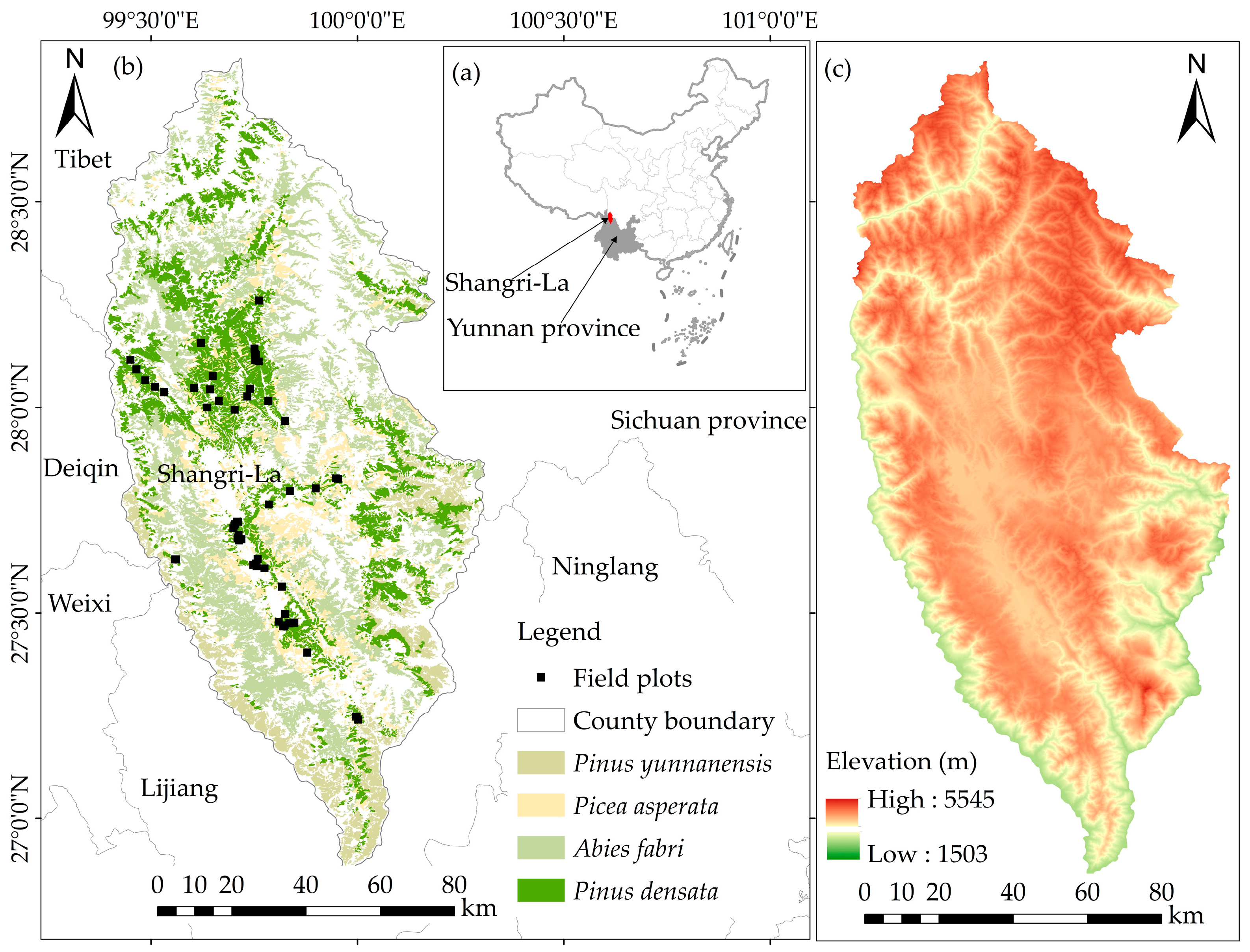
2.1. Study Area and Materials

2.1.1. Study Area

Shangri-La is located in the area of 99°20′~100°19′ E, 26°52′~28°52′ N, the “Three parallel rivers” area of northwestern Yunnan Province, the southwest of China (Figure 1a,b). The southeastern terrain is lower than the northwestern part. The highest point stands at 5545 m above sea level. The lowest point stands at 1503 m above sea level (Figure 1c). Shangri-La has a remarkable monsoon climate, with rainfall concentrated in the months of June to October each year [36]. The average annual precipitation is 268~945 mm, and the annual sunshine is 1742.9~2186.6 h [37]. It is one of only three remaining natural forest areas and a key area for the implementation of the “Tianbao Project” in China. It is also one of the world’s top ten species gene pools and an important part of global biodiversity. It is characterized by cool coniferous forests, temperate coniferous forests, and oak forests [38]. The dominant tree species are Quercus semicarpifolia, Pinus yunnanensis, Pinus densata, Picea asperata, Abies fabri, etc. (Figure 1b). The Pinus densata is endemic to the mountainous regions of the western plateau of China, covering 1848.18 km2, accounting for 16.18% area of Shangri-La [39]. The Pinus densata is an important species in the upper reaches of the Yangtze River region. Therefore, estimating the AGB of Pinus densata holds significant importance in assessing and developing forestry carbon storage in the area.

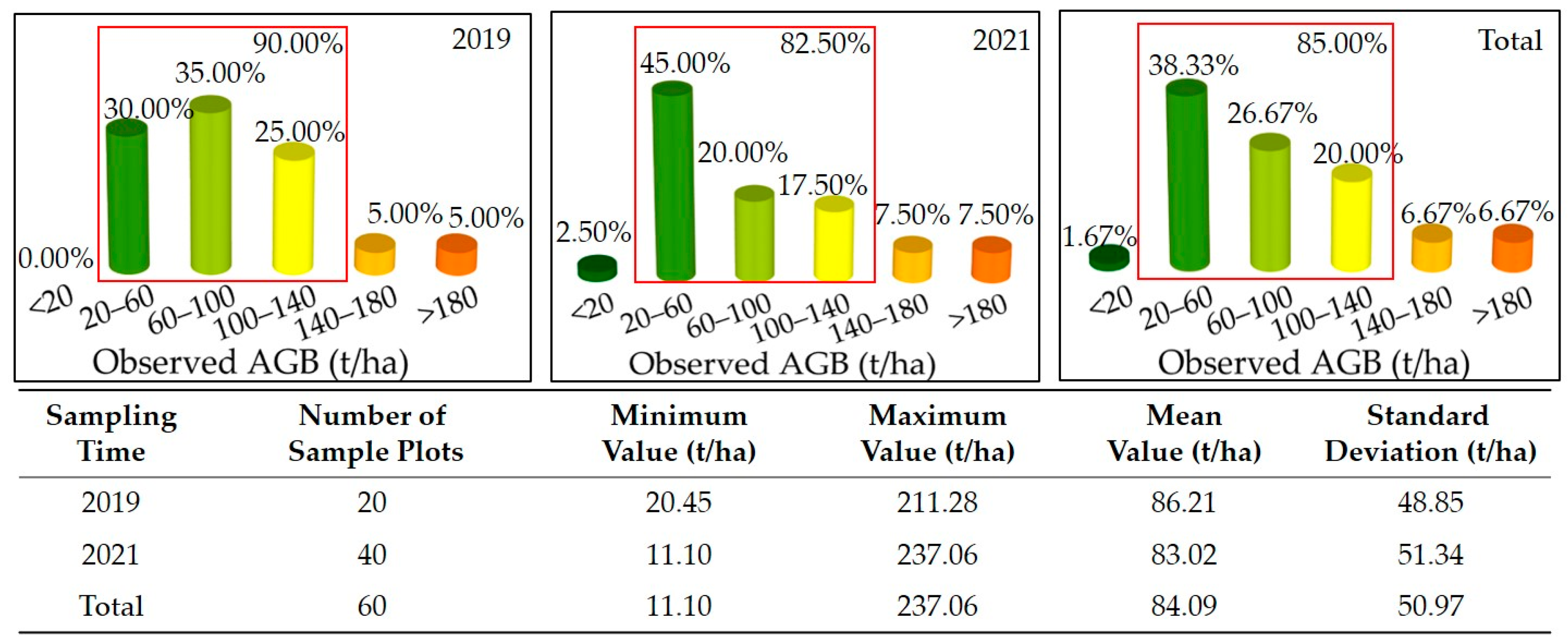
2.1.2. Sampling Design

A total of 60 sample plots of size 10 m × 10 m were surveyed, with 20 of these plots surveyed in December 2019, and the other 40 surveyed in May 2021. Plot sizes of 10 m × 10 m were considered in this study to ensure correspondence between the field measurement and pixel size in the imagery [13].The mean annual growth rates of tree height and diameter at breast height (DBH) per Pinus densata were 1.71 m and 0.01 cm, respectively; the mean annual growth rate of AGB in this area is 0.0001 t/ha [40,41]. Since the estimated annual growth in this area is so small, we did not adjust our field measurements for potential changes that might have occurred between 2019 and 2021. Sample points were randomly distributed in pure Pinus densata forest areas (Figure 1b). The coordinates of plots was recorded in the field with real-time kinematics (RTK). To estimate AGB, we measured the DBH and tree height of per tree with DBH ≥ 5 cm and tree height ≥ 1.3 m. Tree height was measured from the base to the highest tip of the tree to the nearest 0.1 m using a laser rangefinder. The AGB of the individual trees was calculated using the allometric growth equation [42]. The allometric growth equation is as follows:
W = 0.073   ×   D 1.739   ×   H 0.880
where W is the AGB in kg per tree; H = height (m); D = diameter at breast height (cm). The AGB of each sample plot was the sum of the individual trees in the sample plot. Figure 2 presents the summary statistics of observed AGB. Total AGB values ranged from a low of 11.10 t/ha to a high of 237.07 t/ha, with a mean of 84.09 t/ha.

2.1.3. Image Acquisition and Pre-Processing
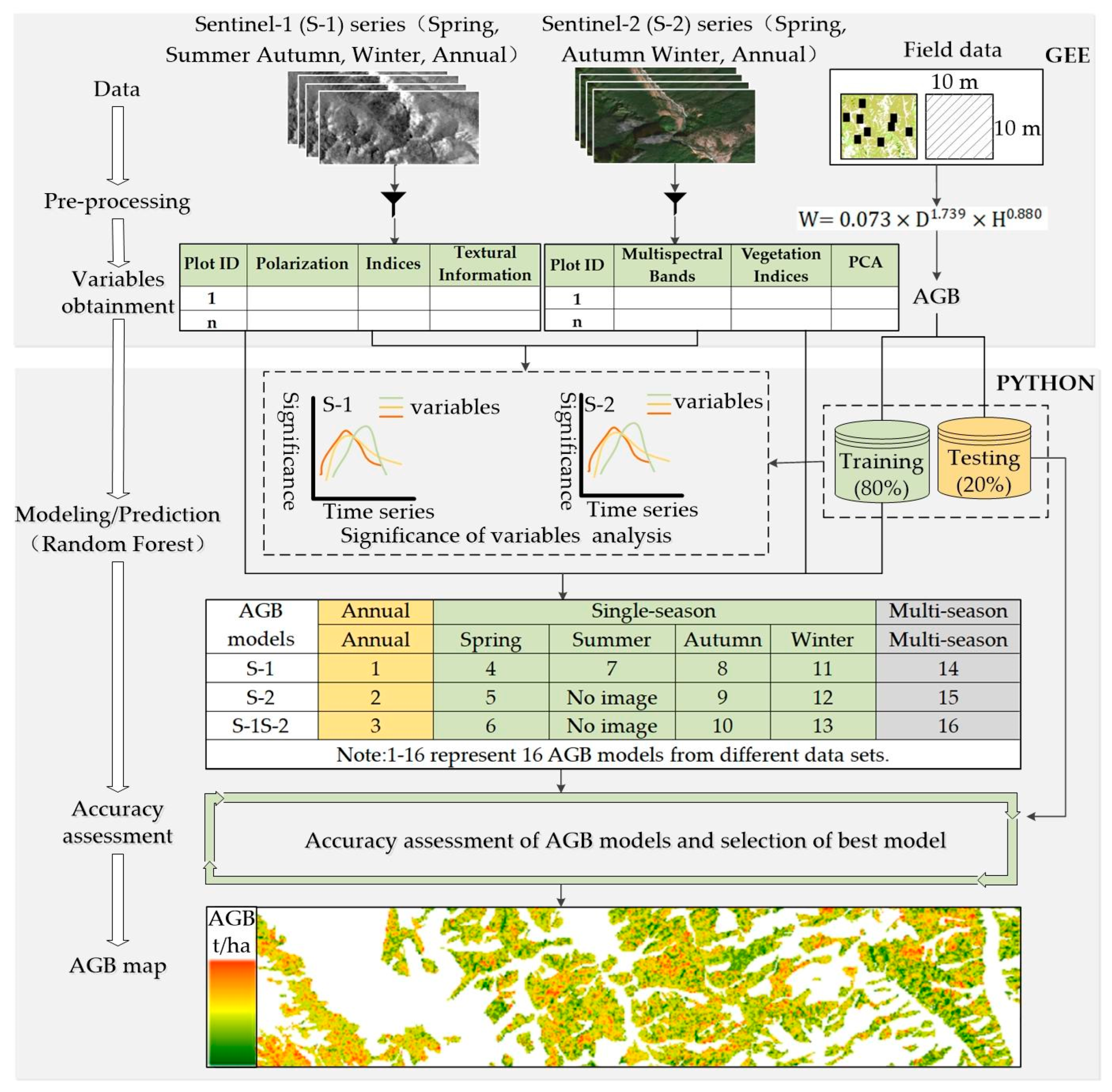
S-1 and S-2 satellite images were obtained from the Copernicus Open Access Hub (COAH, https://scihub.copernicus.eu/ (accessed on 16 May 2023)). The Google Earth Engine (GEE, https://earthengine.google.com/ (accessed on 16 May 2023)) was used to obtain and pre-process images.
S-1 images used in the study were Ground Range Detected (GRD) products from the Wide Swath (IW) with a resolution of 10 m. The orbit property was descending. We used three orbits, and the numbers of relative orbits were 33, 99, and 135. We first acquired images from S-1 during five time periods: spring, summer, autumn, winter, and annual. The S-1 images were processed using Sentinel-1Toolbox (S1TBX) on the GEE platform, which included radiometric calibration, thermal noise reduction, and topographic correction [13]. The backscatter values of the pre-processed image elements were converted into decibels [17]. The equation is as follows:
0 dB = 10   ×   l o g 10 0
where 0 (dB) is the normalized radar cross section and 0   is the backscatter for a specific polarization. The Refined Lee filter of SNAP was used to reduce image noise and upscale data quality [43]. Finally, a median reducer was applied to image collection [44].
We acquired images from S-2 for four time periods: spring, autumn, winter, and annual. Excessive cloud cover in the study area during the summer rendered the images unavailable. Images with less than 10% cloudiness were selected. Images were further pre-processed with an automatic cloud masking procedure using QA bands provided for the S-2 L2A product, masking both opaque and cirrus cloud cover. A median reduction process was performed on the remaining image collection. Finally, the nearest neighbor method was applied to resample the images in the 20 m bands to 10 m [44,45]. Table 1 presents the profile of S-1 and S-2.

2.2. Methodology

In the study, we used S-1 and S-2 time series and sample plots to estimate the AGB of Pinus densata in Shangri-La. Image acquisition, pre-processing, and variable obtainment were based on the GEE. Random Forest (RF) was used to model the AGB. The overall workflow is shown in Figure 3. Five main steps were followed to derive the AGB map: (1) acquisition of muti-source time series images; (2) obtainment of remote sensing variables; (3) modeling; (4) accuracy assessment; (5) AGB mapping.

2.2.1. Multi-Source Time Series Images

In line with the study’s objective, we designed 16 experiments on three time scales: annual, single season, and multi-season (Figure 4).
  • Annual: Annual data were medially synthesized from images during 1 December 2020 and 1 December 2021. There were 3 experiments.
  • Single season: Single seasons included spring, summer, autumn, and winter. The images used for each season were a composite of the median of all images from that season. There were 10 experiments.
  • Multi-season: Multi-seasons were a combination of images from four seasons used in a single season. There were 3 experiments.

2.2.2. Obtainment of Relevant Variables

Numerous studies revealed that backscatter coefficients of SAR were crucial for AGB retrieval [13,17]. Difference (VH − VV), sum (VH + VV), and radar texture information are also significant in AGB retrieval [17,46,47,48]. Hence, we obtained radar backscatter coefficients, differences (VH − VV), sums (VH + VV), and radar texture information from S-1. According to the specific characteristics of the study area, as well as the results of related studies [24,46,49,50], key variables such as the red edge bands, vegetation indices, and the first three principal components were selected from the pre-processed S-2 images. We utilized 10 bands from S-2 for principal component analysis (PCA), excluding atmospheric bands B1, B9, and B10 [51]. Variables selected from S-1 and S-2 are shown in Table 2.

2.2.3. Modeling

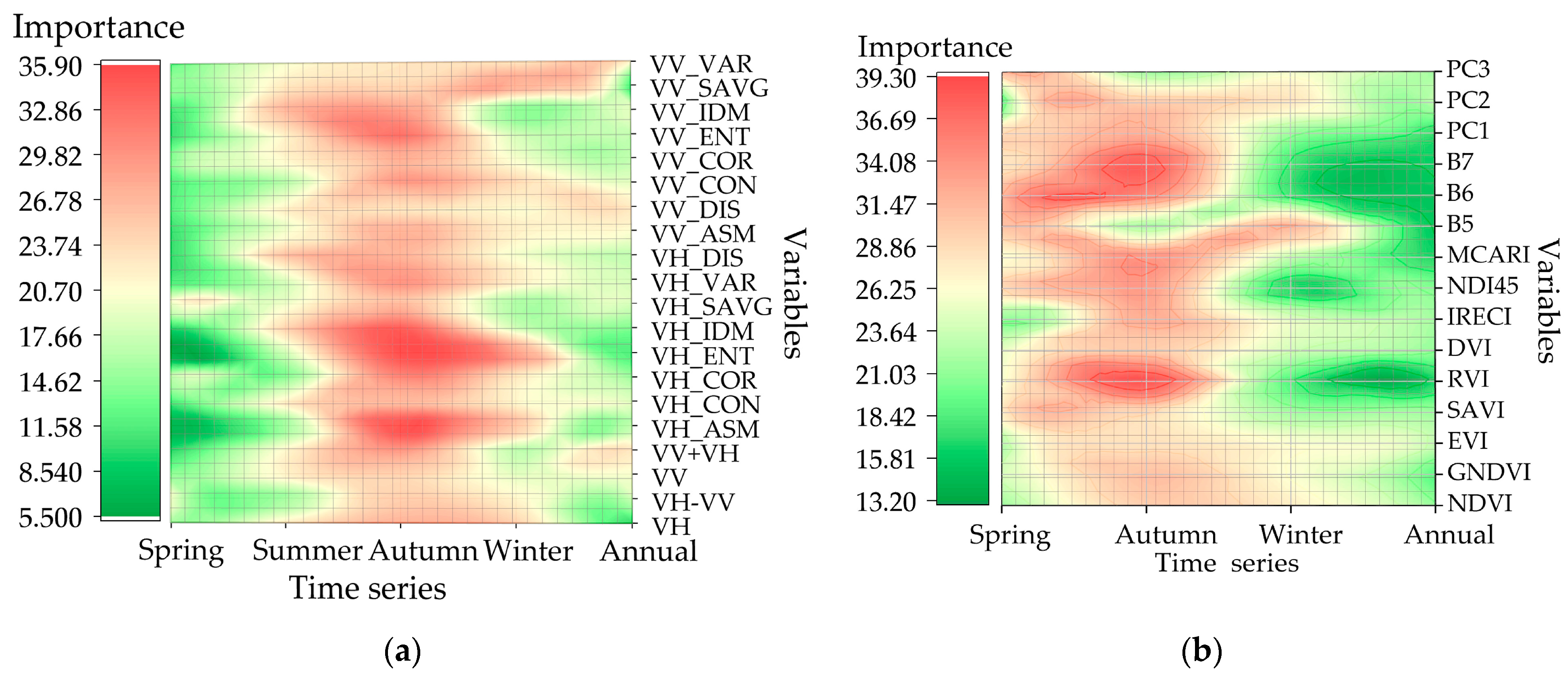
Importance Assessment of Remote Sensing Variables

Variable significance can assess the sensitivity of the argument to the dependent variable. We analyzed the significance of variables at different time periods (spring, summer, autumn, winter, and annual) from S-1 and S-2 using RF. This result will be used to initially determine the sensitivity of the data to AGB for each period.

Selection of Variables Used in AGB Modeling

Experiments involving S-1S-2 and multi-season data had a large number of remote sensing variables with covariance and redundancy. Some variables have a low correlation with AGB, or these variables may be co-dependent. To overcome the challenge of selecting the fewest predictors with the best predictive power and to help in the interpretation of the final model, backward feature elimination (BFE) was used to select appropriate variables [47,52]. Variables used in 16 AGB models are shown in Table 3.

Modeling Method

The Random Forest model is widely used for forest AGB estimation due to its robustness, ability to handle high-dimensional features, and ability to handle complex relationships between independent variables in AGB estimation models [53,54]. The “Random Forest Regressor” algorithm from the Python (3.2) language “sklearn” package was used to conduct this study. The four main parameters in RF are maximum iteration of weak machine learning, maximum depth of the decision tree, minimum number of samples at a leaf node, and minimum number of samples required to split. The maximum iteration of weak machine learning was tested from 20 to 200, and the optimal tuning result was selected based on the stability of the RMSE [55]. When the maximum depth of the decision tree was tuned, the result did not change; so, it was set to 10. We had a small number of sample plots in this study; so, the minimum number of samples at a leaf node was set to 1. The minimum number of samples required to split was set to 2 [56].

2.2.4. Accuracy Assessment

Sixty sample plots were used in this study; eighty percent (48 groups) of the data were randomly selected for model fitting, the remaining 20% (12 groups) were used for validation, and cross-validation was performed during model fitting. We used the coefficient of determination (R2) and root mean square error (RMSE (t/ha)) to assess the model fitting performance on the training dataset. Twenty percent (12 groups) of the data were set apart separately (this portion of data was not involved in model training) for model validation; the accuracy evaluation indicators employed were the relative root mean square error (rRMSE) and the prediction accuracy (p) [57]. To ensure that the model results were as objective as possible, each model was fitted 20 times in this study to allow the mean values of evaluation indicators to be used for comparison [37]. The formulas are as follows:
R 2 = i = 1 n ( y i ^ y ¯ ) 2 i = 1 n ( y i y ¯ ) 2
R M S E = i = 1 n ( y i - y i ^ ) n
r R M S E = R M S E y ¯ × 100 %
p = 1 n i = 1 n 1 - y i - y i ^ y i ^ × 100 %
where n is the number of sample plots, y i   is the observed value, y i ^ is the predicted value, and y ¯ is the mean of the observed values.

3. Results

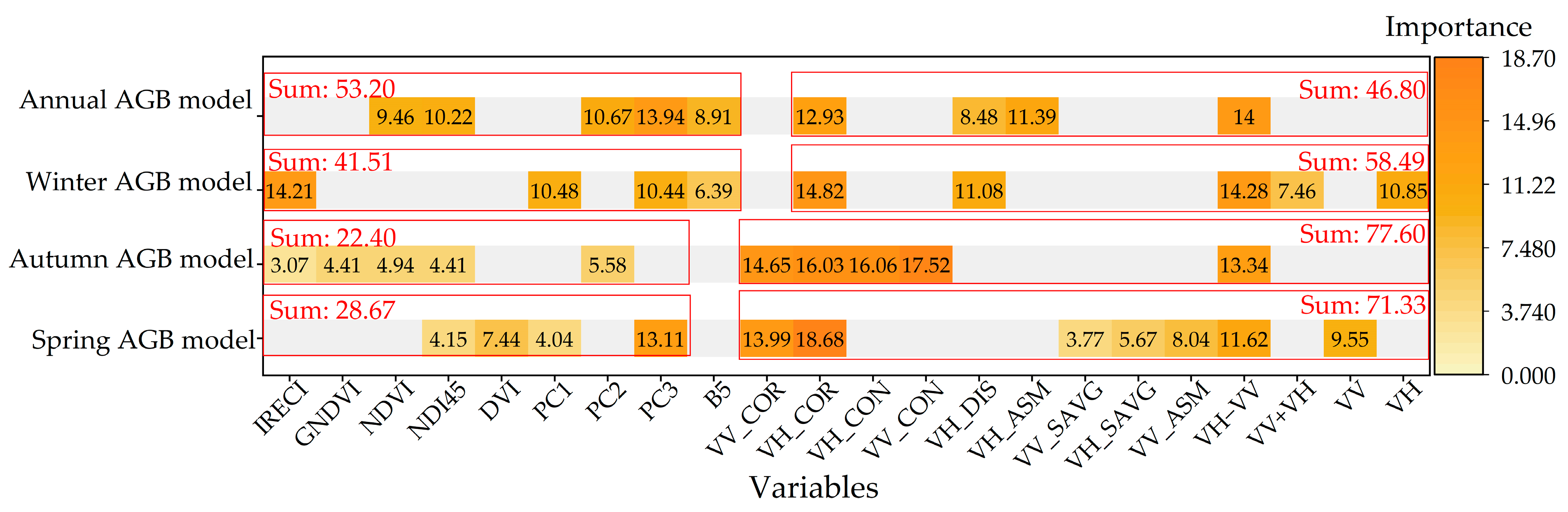
3.1. Significance of Variables

The significance of variables at different time periods is shown in Figure 5. The variables from autumn in S-1 were the most important; the importance of summer, winter, and annual variables was at a medium level; the importance of variables from spring was the lowest. The variables from autumn in S-2 also were the most significant; contrary to S-1, the variables from spring in S-2 were more significant than those from winter and annual. These results showed that the autumn data from S-1 and S-2 had the highest sensitivity to AGB among the single-seasonal and annual data.
Figure 6 shows the importance of the variables of spring, autumn, winter, and annual AGB models from S-1S-2. In four AGB models, the most important variables came from S-1. The most important variable of the spring and winter AGB model was VH_COR; the most important variable of the autumn AGB model was VV_CON; the most important variable of the annual AGB model was VH − VV. In the spring and autumn AGB models, most of the variables from S-1 were more important than those from S-2. In the spring, autumn, and winter AGB models, the sum of the significance of variables from S-1 was higher than that of S-2.
Figure 7 shows the importance of variables of multi-season AGB models. The most important variables came from the autumn in these three multi-seasonal models. In the S-1 AGB model, the importance of variables from different periods was ranked in descending order: autumn, winter, summer, and spring (Figure 7a). In the S-2 AGB model, the importance of the variables at different periods was ranked in descending order: spring, autumn, and winter (Figure 7b). In the S-1S-2 AGB model, the importance of the variables at different periods was ranked in descending order: autumn, spring, and winter (Figure 7c).

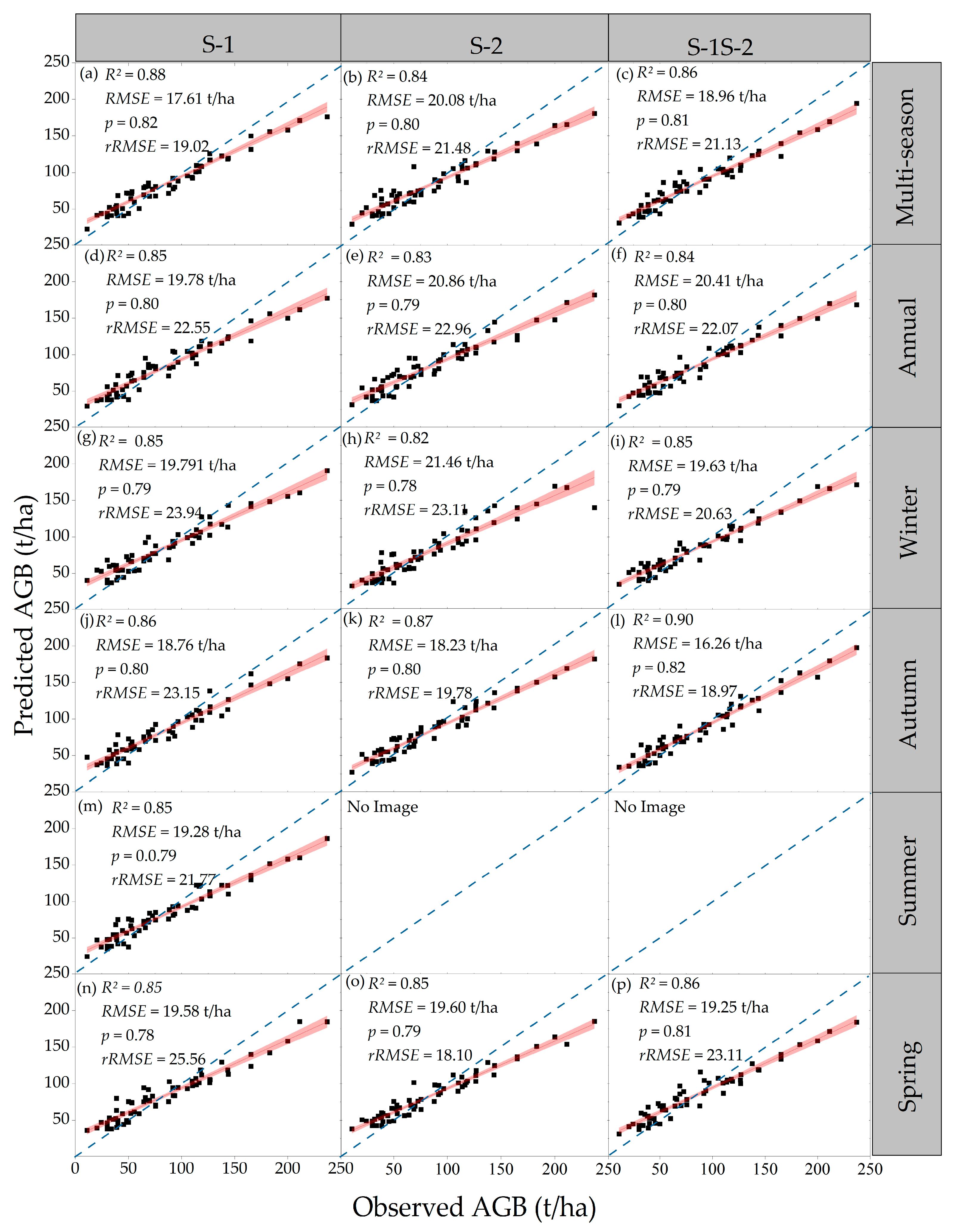
3.2. AGB Models of Periods from S-1, S-2, and S-1S-2

The accuracy assessment results of 16 AGB models are shown in Figure 8. In the 16 models, we found that the AGB model based on autumn images from S-1S-2 was the best (Figure 8l), with R2 = 0.90, RMSE = 16.26 t/ha, p = 0.82, and rRMSE = 18.97.
The estimation accuracy of AGB models from S-1 was ranked in descending order: multi-season, autumn, annual, summer, winter, and spring (Table 4). The estimation accuracies for spring, summer, winter, and annual were relatively close, with R2 of 0.85 and p of 0.78 to 0.80. (Figure 8d, g, m, n). The confidence interval for the multi-season was significantly narrower than those for the single-season or annual at the same confidence level (95%). The multi-season AGB model was best in S-1, with R2 = 0.88, RMSE = 17.61 t/ha, p = 0.82, and rRMSE = 19.02 (Figure 8a). Overall, the quality of images from S-1 was relatively consistent. The estimation accuracy of AGB models from S-2 was ranked in descending order: autumn, multi-season, spring, annual, and winter (Table 4). The AGB model established with autumn data had the best performance, with R2 = 0.87, RMSE = 18.23 t/ha p = 0.80, and rRMSE = 19.78 (Figure 8k). The multi-season had higher estimation accuracy than annual, spring, and winter (Figure 8b, e, h, o). The estimation accuracies of multi-season and spring were similar in S-2 (Figure 8b, o). The estimation accuracy of AGB models from S-1S-2 was ranked in descending order: autumn, multi-season, spring, annual, and winter (Table 4). The AGB model of autumn data was the best, with R2 = 0.90, RMSE = 16.26 t/ha, p = 0.82, and rRMSE = 18.97 (Figure 8l). The multi-season and spring AGB models in S-1S-2 had relatively similar estimation accuracy, R2 = 0.86, p = 0.81; however, the RMSE and rRMSE of the multi-season were smaller than the spring (Figure 8c, p).
The ability of S-1 to estimate AGB was better than that of S-2 in winter, summer, annual, and multi-season (Figure 8a, b, d, e, g, h, m). However, in autumn and spring, the estimation accuracy of S-2 differed less than that of S-1, and the estimation accuracy exceeded S-1 (Figure 8j, k, n, o). Compared with S-1, S-1S-2 improved the estimation accuracy in spring and autumn (Figure 8j, l, n, p); in winter, annual, and multi-season, S-1S-2 did not improve the estimation accuracy (Figure 8a, c, d, f, g, i). Compared to S-2, S-1S-2 somewhat improved estimation accuracy in all periods (Figure 8b, c, e, f, h, i, k, l, o, p).

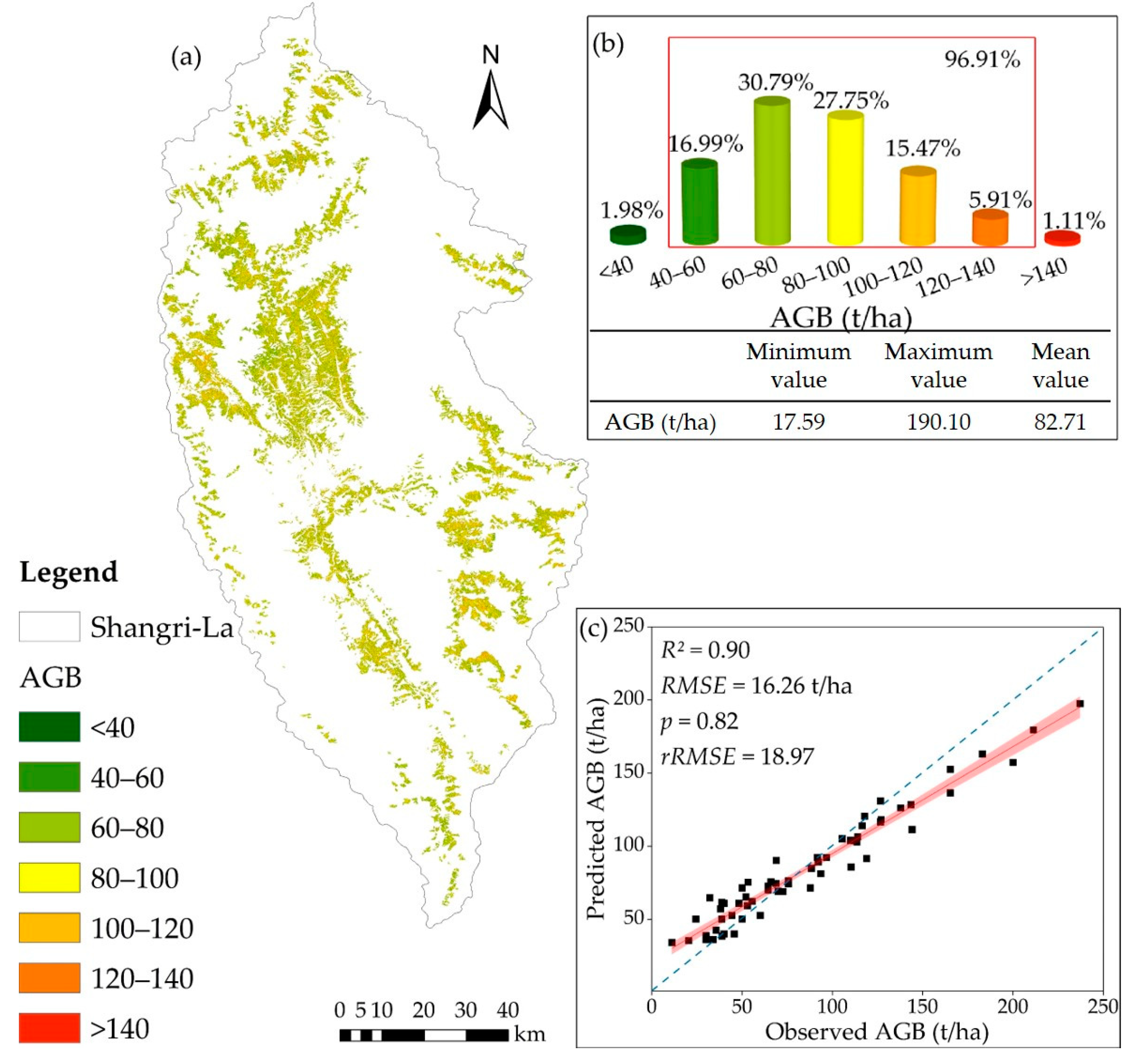
3.3. Spatial Distribution of Pinus Densata AGB

Based on estimation accuracy, the AGB model with the highest accuracy from S-1S-2 was used to estimate the AGB of Pinus densata. Figure 9a depicts the spatial distribution of AGB of Pinus densata. Figure 9b depicts the percentage of plots and pixels occurring in different AGB classes. The range of AGB was from 17.59 t/ha to 190.10 t/ha, with a mean of 82.71 t/ha. The total AGB was 17.21 million tons. Thirty point seven nine percent of the area was characterized by AGB values between 80 and 100 t/ha. Overall, ninety-six point nine one percent of the area had AGB values of 40–140 t/ha.
The topography of the area is complex. We analyzed the spatial distribution characteristics of the AGB of Pinus densata in terms of elevation, slope, and aspect perspectives. The slope was classified into six classes (Figure 10a) according to the method of grading slopes in forestry [30]. Based on the topographic characteristics of the area [30], we divided the elevation into seven classes (Figure 10b). The aspect was classified into nine classes (Figure 10c) according to the method of grading slopes in forestry [42].
Regarding slope, most AGB was found on slopes ranging from 6° to 45°, i.e., gentle, moderate, steep, and very steep slopes. Of these, thirty point six three percent of AGB was found on moderate slope; and thirty-two point five eight percent of AGB was found on steep slopes. It was not easy to find AGB on flat and extremely steep slopes; the sum of flat and extremely steep slopes was 5%. Overall, there was a normal distribution pattern. Across gentle, moderate, and steep slopes, the percentage of AGB was higher than the percentage of the area, indicating a denser distribution of Pinus densata in these regions. In terms of elevation, the AGB of Pinus densata was mainly concentrated between 2400–4000 m, accounting for 99.69% of the total AGB. Over half of the AGB could be found between 3200–3600 m, accounting for 56.54% of the total AGB. Secondly, the AGB was mainly found at 2800–3200 m altitudes, accounting for 28.46% of the total AGB. At 2800–3600 m, the percentage of AGB greatly exceeded the percentage of the area, showing that the density of Pinus densata was high and that it was the dominant tree species in the area. The area above an elevation of 4000 m accounted for 23.67% of the total area; however, the percentage of AGB was only 0.28%. As far as the aspect was concerned, AGB was more evenly distributed across aspects. The area was dominated by mountainous terrain; fewer areas were flat. Except for the flat area, the northwestern aspect contained the least, accounting for 5.42% of the total AGB, while the AGB of the eastern was the most, accounting for 21.67% of the total AGB. The percentage of AGB for each aspect didn’t differ significantly from the percentage of the area.

4. Discussion

4.1. Effect of Seasonality on Data Selection

All experiments involving S-1 have shown that autumn data had greater potential for AGB estimation than spring, summer, autumn, and winter. Despite the strong penetration and all-weather imaging capability of SAR, seasonal changes could cause changes in vegetation canopy thickness, vegetation water content, soil moisture content, and other factors affecting the sensitivity of SAR to AGB [22,58]. Most of the C-band’s backscatter coefficient comes from the top of the forest canopy [59]. Pinus densata, an evergreen needle-leaved forest, is less affected by seasonal defoliation [24] and is mainly influenced by the water content of vegetation, soil, etc. The rainy season in Shangri-La is primarily during the summer, which coincides with the peak season of vegetation, but the water content is also very high during this season. Most of the Pinus densata are found at middle and high altitudes covered by snow for long periods in winter, with low temperatures and low evaporation. This area’s vegetation and soil water content is relatively high. Thus, the winter and summer images were less valid for AGB estimation than the autumn. Our findings agree with previous studies [17,60], which also suggested limitations in using SAR data for AGB estimation during the rainy season. For the optical data, images from autumn are less affected by the weather. Autumn is the end of the growing season of Pinus densata. Therefore, the autumn AGB model from S-2 was the best. Maselli et al. [61] and Wallner et al. [62] also identified that using optical data from the beginning or the end of the growing season improved prediction ability. During the wet season, summer, optical data are affected by clouds and rain, making it difficult to obtain complete images. In winter, as Shangri-La is a high-altitude area, snow will affect image quality.
Whether S-1, S-2, or S-1S-2, the accuracy of the annual AGB model was lower than that of multi-season and autumn models. This finding agrees with a previous study [24]. The annual data was the median of the total yearly images. The quality of the median composite image depends on the quality of the input image. The quality of some of the total yearly images was poor, which decreased the quality of the composition image. In addition, it is difficult for annual data to capture seasonal information. As a result, the ability of the annual images to estimate AGB was weaker than that of optimal seasonal and multi-seasonal images.
In S-1, the multi-season AGB model had the highest estimation accuracy. Castillo et al. [63] considered this an effective approach to improve accuracy using multi-temporal (acquired in January, October, and November) data from S-1. In S-2, the accuracy of the multi-seasonal model was higher than that of spring, winter, and annual. Furthermore, when combining S-1 and S-2, the result was consistent with those obtained using S-2 only. Our findings are similar to previous studies [19,64]. Zhu and Liu [32] also concluded that multi-temporal data could improve the estimation accuracy of AGB. The reason the accuracy of the autumn models from S-2 and S-1S-2 was higher than that of the multi-season could be that the multi-seasonal model was influenced by poor quality data from S-2, namely winter and summer. In contrast, the quality of SAR images is more stable and less affected.
According to Figure 6, Figure 7 and Figure 8, SAR outperformed optical sensors. However, in spring and autumn, when images were relatively less affected by clouds, rain, and snow, the difference between the sensitivity of S-1 and S-2 to AGB was decreased, and the estimation accuracy of S-2 even exceeded that of S-1. Zhang et al. [14] used S-1 and S-2 to assess the AGB of arid ecosystems in the Sahel. They found that S-1 demonstrated better performance than S-2; however, it also led to an overestimation of AGB in the region. Zhao et al. [18] and Vafaei et al. [16] obtained the opposite results, demonstrating that optical sensing was superior to SAR. Therefore, the sensitivity of SAR and optical remote sensing to AGB may be affected by climatic and geographical conditions, leading to diverse outcomes. Numerous studies found that integrating SAR with optical sensing could enhance AGB estimation accuracy to a certain degree [13,17,65]. In this study, the combination of S-1 and S-2 improved the estimation accuracy compared to S-2; compared to S-1, only the combination of S-1 and S-2 in spring or autumn could improve the estimation accuracy.
In this study, the variables obtained from the four seasons were directly used to establish the multi-season AGB model without data fusion. Therefore, the accuracy of the multi-season AGB model might be limited for data with less stable data quality, such as S-2. Next, we will further explore the effective fusion of multi-seasonal data.

4.2. Comparison with Existing Results

In this study, S-1S-2 was used for the first time to estimate the AGB of Pinus densata in Shangri-La. The mean estimated AGB was 82.71 t/ha, which differed from the mean observed AGB by only 1.38 t/ha. The elevation, slope, and direction distribution patterns were roughly the same as in previous studies [30,38,42]. The AGB of this study reached 17.21 million tons.
Total AGB varied among researchers due to differences in remote sensing data, sample plots, and estimation methods. Figure 11 summarizes the estimation results of the Pinus densata from different researchers. Some studies have shown that AGB accounted for about 70%–90% of forest biomass, and under-ground biomass accounted for about 4%–8% [2,66]. So, it could be inferred that the AGB of Pinus densata in the study of Wang et al. [30] was 14~18 million tons. Yue [38] combined Landsat imagery with 50 sample plots to estimate the AGB of Pinus densata in Shangri-La; the AGB was 13.02~13.41 million tons in 2008. Xie [67] combined Landsat imagery with 50 sample plots and utilized the K-NN algorithm to estimate the AGB of the area; the AGB of Pinus densata was 15.75–20.25 million tons in 2015. Sun [42] combined Landsat data with 56 sample plots and utilized the RF model to estimate the AGB. The results indicated that in 2014, the AGB was 11.72 million tons. We calculated the AGB of Pinus densata in Shangri-La using the forest management investigation data (category II of forest inventory); in 2016, the AGB was 14.9 million tons. In addition, several researchers [26,27,68] studied the AGB dynamics of Pinus densata in the region using Landsat time series imagery. Their study showed that the AGB ranged from 7–10 million tons from 1985 to 2017. They used ground survey data from the National Forestry Inventory of China. The distance between the sample plots consisted of regular distributions of 6 km × 8 km. The sample plots were established in a grid pattern at fixed distances (6 km × 8 km), without taking into account forest density and forest type. Some of the sample plots might be established in areas with lower forest density or within mixed forests. However, they only investigated information from Pinus densata, excluding other tree species within plots. Hence, the AGB was smaller than other studies. In this study, we randomly placed the sample plots in pure Pinus densata forest areas based on the subcompartment data from the forest management investigation. However, due to the complex terrain in Shangri-La, the location of certain sample plots was situated in areas with steep topography, which posed challenges for data measurement. The location of these specific sample plots was determined artificially. These sample plots artificially selected might tend to be distributed in areas of higher forest density. Thus, the value of the AGB was relatively high. In addition, the “returning farmland to forest” policy was implemented in Shangri-La in 2000 [26]. After 21 years of forest cultivation, young forests gradually grew into middle-aged and mature woodland, leading to an increase in AGB.

4.3. Sensitive Analyses of the Model

Observed AGB measurements are relatively labor intensive to produce. Therefore, the number of sample plots used in the AGB estimation studies is often small. Fassnacht et al. [69] compiled the number of sample plots from 113 relevant studies. Out of these 113 studies, 66 studies had fewer than 100 sample plots, and the number of samples of 51 studies was between 20 and 60. Furthermore, due to the size and characteristics of the study area, many studies focusing on AGB conducted in that region had a relatively small number of sample plots [39,67,70,71].
To further validate the results, we conducted the sensitivity analysis of the RF model using the bootstrap approach. Bootstrapping entails resampling from the original sample data and mimicking the original sampling, which helps evaluate the original sample [72,73]. We selected 100 bootstrap samples by repeatedly resampling. The number of bootstrap sample plots was 80% (48 groups) of that of the original samples. Each bootstrap sample was utilized to establish the AGB model. The variables used in the modeling were consistent with that of the optimal AGB model. Eighty percent (38 groups) of the data were randomly selected for model fitting and the remaining 20% (10 groups) were used for validation. We used R2 and RMSE to assess the model-fitting performance on the training dataset, p and rRMSE to assess the model-fitting performance on the test dataset. The result of 100 bootstrap sample AGB models is presented in Figure 12. The mean values of evaluation indicators of the bootstrap sample AGB models were R2 = 0.88, RMSE = 17.55 t/ha, p = 0.81, and rRMSE = 20.46. Compared to the optimal AGB model, R2 decreased by 0.02, RMSE increased by 1.29 t/ha, p decreased by 0.01, and rRMSE increased by 1.49. However, the accuracy was still higher than that of other original sample AGB models. In addition, the distribution of evaluation indicators in the boxplots was relatively concentrated, which indicates that the model was relatively stable and our study results were reliable. However, the evaluation indicators of the model still have some fluctuations. In the future, researchers may consider further exploring ways to improve the stability of the model and the accuracy of AGB estimation.

5. Conclusions

Overall, the estimation accuracy of the autumn AGB model from S-1S-2 was the highest. The estimation accuracy of the multi-seasonal AGB model from S-1 exceeded that of the single seasonal and annual; the estimation accuracy of the autumn AGB model, whether from S-2 or S-1S-2, was the highest. Future researchers could use multi-seasonal SAR data and optical data from the best season to improve the AGB estimation accuracy. The ability of S-1, S-2, and S-1S-2 to estimate AGB was ranked in descending order: S-1, S-1S-2, S-2 with winter, summer, annual, and multi-seasonal images; in spring and autumn, the order was: S-1S-2, S-1, S-2. Therefore, we should use seasonal characteristics to determine whether to use single-source or multi-source data in different time scales.
Ninety-six point nine one percent of the area was characterized by the AGB of 40–140 t/ha; the AGB was greater than 140 t/ha or less than 40 t/ha in a few areas. The value ranges indicated that Shangri-La was generally characterized by high AGB values. Proper planning, management, and use of the area’s forest resources are conducive to achieving carbon peak and carbon neutrality.
Clouds, rain, and snow are the key factors limiting the estimation of AGB using remote sensing imagery. Considering seasonal effects is essential to conquer the limitations. We found the optimal time scales of S-1, S-2, and S-1S-2 images for AGB estimation and the ability of different data to estimate AGB in different phenological conditions. This result will help improve forest resource monitoring and management in subtropical forest areas with monsoon climate characteristics. At the same time, it also can provide a scientific basis and decision-making support for ecological protection and economic development.

Author Contributions

C.C. participated in the data analysis and wrote the draft article, Y.H. helped with the data analysis, J.Z. helped with the idea and draft revision, and D.X., D.H., Y.L., L.L., C.T. and T.Y. participated in the draft revision. All authors have read and agreed to the published version of the manuscript.

Funding

This research was funded by the “Young Top Talents” special project of the high-level talent training support program of Yunnan province, China, in 2020 (No. YNWR-QNBJ-2020-164) and the National Natural Science Foundation of China (Nos. 32260390 and 31860207).

Data Availability Statement

The Sentinel-1 and 2 simulated data are available through https://earthengine.google.com/ (accessed on 16 May 2023) and https://scihub.copernicus.eu/ (accessed on 16 May 2023). Sample plots presented in this study are available on request from the corresponding author; the data are not publicly available due to the confidentiality of the dataset.

Acknowledgments

We would like to thank the editor and anonymous reviewers for their comments, which helped improve the manuscript. We thank the Copernicus Open Access Hub for free remote sensing imagery and the Google Earth Engine for providing the platform and algorithmic support for our data acquisition and processing. We also would like to acknowledge all the other individuals who contributed to this paper.

Conflicts of Interest

The authors declare no conflict of interest.

References

  1. Liu, K.; Wang, J.; Zeng, W.; Song, J. Comparison and Evaluation of Three Methods for Estimating Forest above Ground Biomass Using TM and GLAS Data. Remote Sens. 2017, 9, 341. [Google Scholar] [CrossRef]
  2. Chave, J.; Andalo, C.; Brown, S.; Cairns, M.A.; Chambers, J.Q.; Eamus, D.; Fölster, H.; Fromard, F.; Higuchi, N.; Kira, T.; et al. Tree Allometry and Improved Estimation of Carbon Stocks and Balance in Tropical Forests. Oecologia 2005, 145, 87–99. [Google Scholar] [CrossRef] [PubMed]
  3. Cairns, M.A.; Brown, S.; Helmer, E.H.; Baumgardner, G.A. Root Biomass Allocation in the World’s Upland Forests. Oecologia 1997, 111, 1–11. [Google Scholar] [CrossRef]
  4. Lu, D.; Chen, Q.; Wang, G.; Liu, L.; Li, G.; Moran, E. A Survey of Remote Sensing-Based Aboveground Biomass Estimation Methods in Forest Ecosystems. Int. J. Digit. Earth 2016, 9, 63–105. [Google Scholar] [CrossRef]
  5. Lu, D. The Potential and Challenge of Remote Sensing-based Biomass Estimation. Int. J. Remote Sens. 2006, 27, 1297–1328. [Google Scholar] [CrossRef]
  6. Houghton, R.A.; Hall, F.; Goetz, S.J. Importance of Biomass in the Global Carbon Cycle. J. Geophys. Res. Biogeosci. 2009, 114, G00E03-1–G00E03-13. [Google Scholar] [CrossRef]
  7. Campos-Taberner, M.; Moreno-Martinez, A.; Garcia-Haro, F.; Camps-Valls, G.; Robinson, N.; Kattge, J.; Running, S. Global Estimation of Biophysical Variables from Google Earth Engine Platform. Remote Sens. 2018, 10, 1167. [Google Scholar] [CrossRef]
  8. Puliti, S.; Breidenbach, J.; Schumacher, J.; Hauglin, M.; Klingenberg, T.F.; Astrup, R. Above-Ground Biomass Change Estimation Using National Forest Inventory Data with Sentinel-2 and Landsat. Remote Sens. Environ. 2021, 265, 112644. [Google Scholar] [CrossRef]
  9. Berninger, A.; Lohberger, S.; Zhang, D.; Siegert, F. Canopy Height and Above-Ground Biomass Retrieval in Tropical Forests Using Multi-Pass X- and C-Band Pol-InSAR Data. Remote Sens. 2019, 11, 2105. [Google Scholar] [CrossRef]
  10. Balzter, H. Forest Mapping and Monitoring with Interferometric Synthetic Aperture Radar (InSAR). Prog. Phys. Geogr. Earth Environ. 2001, 25, 159–177. [Google Scholar] [CrossRef]
  11. Kellndorfer, J.M.; Walker, W.S.; LaPoint, E.; Kirsch, K.; Bishop, J.; Fiske, G. Statistical Fusion of Lidar, InSAR, and Optical Remote Sensing Data for Forest Stand Height Characterization: A Regional-Scale Method Based on LVIS, SRTM, Landsat ETM+, and Ancillary Data Sets. J. Geophys. Res. Biogeosci. 2010, 115, G00E08-1–G00E08-10. [Google Scholar] [CrossRef]
  12. Zimbres, B.; Rodríguez-Veiga, P.; Shimbo, J.Z.; da Conceição Bispo, P.; Balzter, H.; Bustamante, M.; Roitman, I.; Haidar, R.; Miranda, S.; Gomes, L.; et al. Mapping the Stock and Spatial Distribution of Aboveground Woody Biomass in the Native Vegetation of the Brazilian Cerrado Biome. For. Ecol. Manag. 2021, 499, 119615. [Google Scholar] [CrossRef]
  13. David, R.M.; Rosser, N.J.; Donoghue, D.N.M. Improving above Ground Biomass Estimates of Southern Africa Dryland Forests by Combining Sentinel-1 SAR and Sentinel-2 Multispectral Imagery. Remote Sens. Environ. 2022, 282, 113232. [Google Scholar] [CrossRef]
  14. Zhang, W.; Brandt, M.; Wang, Q.; Prishchepov, A.V.; Tucker, C.J.; Li, Y.; Lyu, H.; Fensholt, R. From Woody Cover to Woody Canopies: How Sentinel-1 and Sentinel-2 Data Advance the Mapping of Woody Plants in Savannas. Remote Sens. Environ. 2019, 234, 111465. [Google Scholar] [CrossRef]
  15. Chen, L.; Wang, Y.; Ren, C.; Zhang, B.; Wang, Z. Optimal Combination of Predictors and Algorithms for Forest Above-Ground Biomass Mapping from Sentinel and SRTM Data. Remote Sens. 2019, 11, 414. [Google Scholar] [CrossRef]
  16. Vafaei, S.; Soosani, J.; Adeli, K.; Fadaei, H.; Naghavi, H.; Pham, T.D.; Tien Bui, D. Improving Accuracy Estimation of Forest Aboveground Biomass Based on Incorporation of ALOS-2 PALSAR-2 and Sentinel-2A Imagery and Machine Learning: A Case Study of the Hyrcanian Forest Area (Iran). Remote Sens. 2018, 10, 172. [Google Scholar] [CrossRef]
  17. Forkuor, G.; Benewinde Zoungrana, J.-B.; Dimobe, K.; Ouattara, B.; Vadrevu, K.P.; Tondoh, J.E. Above-Ground Biomass Mapping in West African Dryland Forest Using Sentinel-1 and 2 Datasets—A Case Study. Remote Sens. Environ. 2020, 236, 111496. [Google Scholar] [CrossRef]
  18. Zhao, P.; Lu, D.; Wang, G.; Liu, L.; Li, D.; Zhu, J.; Yu, S. Forest Aboveground Biomass Estimation in Zhejiang Province Using the Integration of Landsat TM and ALOS PALSAR Data. Int. J. Appl. Earth Obs. Geoinf. 2016, 53, 1–15. [Google Scholar] [CrossRef]
  19. Chrysafis, I.; Mallinis, G.; Tsakiri, M.; Patias, P. Evaluation of Single-Date and Multi-Seasonal Spatial and Spectral Information of Sentinel-2 Imagery to Assess Growing Stock Volume of a Mediterranean Forest. Int. J. Appl. Earth Obs. Geoinf. 2019, 77, 1–14. [Google Scholar] [CrossRef]
  20. Culbert, P.D.; Pidgeon, A.M.; St.-Louis, V.; Bash, D.; Radeloff, V.C. The Impact of Phenological Variation on Texture Measures of Remotely Sensed Imagery. IEEE J. Sel. Top. Appl. Earth Obs. Remote Sens. 2009, 2, 299–309. [Google Scholar] [CrossRef]
  21. Zhang, L.; Zhang, X.; Shao, Z.; Jiang, W.; Gao, H. Integrating Sentinel-1 and 2 with LiDAR Data to Estimate Aboveground Biomass of Subtropical Forests in Northeast Guangdong, China. Int. J. Digit. Earth 2023, 16, 158–182. [Google Scholar] [CrossRef]
  22. Guccione, P.; Lombardi, A.; Giordano, R. Assessment of Seasonal Variations of Radar Backscattering Coefficient Using Sentinel-1 Data. In Proceedings of the 2016 IEEE International Geoscience and Remote Sensing Symposium (IGARSS), Beijing, China, 10–15 July 2016; pp. 3402–3405. [Google Scholar]
  23. Wu, D.; Li, B.; Yang, A. Estimation of tree height and biomass based on long time serises data of Landsat. Eng. Sur Veying Mapp. 2017, 26, 1–5. [Google Scholar] [CrossRef]
  24. Laurin, G.V.; Balling, J.; Corona, P.; Mattioli, W.; Papale, D.; Puletti, N.; Rizzo, M.; Truckenbrodt, J.; Urban, M. Above-Ground Biomass Prediction by Sentinel-1 Multitemporal Data in Central Italy with Integration of ALOS2 and Sentinel-2 Data. J. Appl. Remote Sens. 2018, 12, 016008. [Google Scholar] [CrossRef]
  25. Ni, W.; Yu, T.; Pang, Y.; Zhang, Z.; He, Y.; Li, Z.; Sun, G. Seasonal Effects on Aboveground Biomass Estimation in Mountain ous Deciduous Forests Using ZY-3 Stereoscopic Imagery. Remote Sens. Environ. 2023, 289, 113520. [Google Scholar] [CrossRef]
  26. Liao, Y.; Zhang, J.; Bao, R.; Xu, D.; Wang, S.; Han, D. Estimation of aboveground biomass dynamics of Pinus densata by introducing topographic factors. Chin. J. Ecol. 2023, 42, 1243–1252. [Google Scholar] [CrossRef]
  27. Zhang, J.; Lu, C.; Xu, H.; Wang, G. Estimating Aboveground Biomass of Pinus Densata-Dominated Forests Using Landsat Time Series and Permanent Sample Plot Data. J. For. Res. 2019, 30, 1689–1706. [Google Scholar] [CrossRef]
  28. Huang, J.; Shu, Q.; Xi, L.; Sun, Y.; Liu, Y. Research on biomass estimation model for Pinus densata based on hierar-chical Bayesian method. Jiangsu J. Agric. Sci. 2022, 38, 1265–1271. [Google Scholar]
  29. Santoro, M.; Cartus, O.; Fransson, J.E.S. Dynamics of the Swedish Forest Carbon Pool between 2010 and 2015 Estimated from Satellite L-Band SAR Observations. Remote Sens. Environ. 2022, 270, 112846. [Google Scholar] [CrossRef]
  30. Wang, J.; Cheng, P.; Xu, S.; Wang, X.; Cheng, F. Forest biomass estimation in Shangri-La based on the remote sensing. J. Zhejiang A & F Univ. 2013, 30, 325–329. [Google Scholar]
  31. Cartus, O.; Santoro, M. Exploring Combinations of Multi-Temporal and Multi-Frequency Radar Backscatter Observations to Estimate above-Ground Biomass of Tropical Forest. Remote Sens. Environ. 2019, 232, 111313. [Google Scholar] [CrossRef]
  32. Zhu, X.; Liu, D. Improving Forest Aboveground Biomass Estimation Using Seasonal Landsat NDVI Time-Series. ISPRS J. Photogramm. Remote Sens. 2015, 102, 222–231. [Google Scholar] [CrossRef]
  33. Periasamy, S. Significance of Dual Polarimetric Synthetic Aperture Radar in Biomass Retrieval: An Attempt on Sentinel-1. Remote Sens. Environ. 2018, 217, 537–549. [Google Scholar] [CrossRef]
  34. Theofanous, N.; Chrysafis, I.; Mallinis, G.; Domakinis, C.; Verde, N.; Siahalou, S. Aboveground Biomass Estimation in Short Rotation Forest Plantations in Northern Greece Using ESA’s Sentinel Medium-High Resolution Multispectral and Radar Imaging Missions. Forests 2021, 12, 902. [Google Scholar] [CrossRef]
  35. Pu, R.; Landry, S. Evaluating Seasonal Effect on Forest Leaf Area Index Mapping Using Multi-Seasonal High Resolution Sat ellite Pléiades Imagery. Int. J. Appl. Earth Obs. Geoinf. 2019, 80, 268–279. [Google Scholar] [CrossRef]
  36. Pan, J.; Wang, J.; Gao, F.; Liu, G. Quantitative Estimation and Influencing Factors of Ecosystem Soil Conservation in Shangri-La, China. Geocarto Int. 2022, 37, 14828–14842. [Google Scholar] [CrossRef]
  37. Liao, Y.; Zhang, J.; Bao, R.; Xu, D.; Han, D. Modelling the Dynamics of Carbon Storages for Pinus densata Using Landsat Images in Shangri-La Considering Topographic Factors. Remote Sens. 2022, 14, 6244. [Google Scholar] [CrossRef]
  38. Yue, C. Forest Biomass Estimation in Shangri-La County Based on Remote Sensing. Ph.D. Thesis, Beijing Forestry University, Beijing, China, 2012. [Google Scholar]
  39. Han, D.; Zhang, J.; Yang, J.; Wang, S.; Feng, Y. Establishment of the remote sensing estimation model of the above-ground biomass of Pinus densata Mast. considering topographic effects. J. Cent. South Univ. For. Technol. 2022, 42, 12–21+67. [Google Scholar] [CrossRef]
  40. Wang, C.; Wang, J.; Jiang, H. Morphological Characteristics of Stem of Pinus yunnanensis and Its Related Speciesin Different Habitats. J. West China For. Sci. 2009, 38, 23–27+125. [Google Scholar] [CrossRef]
  41. Zhang, Y.; Shu, Q.; Xu, Y.; Li, S.; Wang, Y. Study on Optimal Height-Curve Model of Natural Pinus densata Forest in Shan gri-La. For. Resour. Manag. 2016, 46–51. [Google Scholar] [CrossRef]
  42. Sun, X. Biomass Estimation Model of Pinus densata Forests in Shangri-La City Based on Landsat8-OLI by Remote Sensing. Master’s Thesis, Southwest Forestry University, Kunming, China, 2016. [Google Scholar]
  43. Lee, J.-S.; Pottier, E. Polarimetric Radar Imaging: From Basics to Applications, 1st ed.; CRC Press: Boca Raton, FL, USA, 2009; ISBN 978-1-4200-5497-2. [Google Scholar]
  44. Feyen, J.; Wip, G.; Crabbe, S.; Wortel, V.; Sari, S.P.; Van Coillie, F. Mangrove Species Mapping and Above-Ground Biomass Estimation in Suriname Based on Fused Sentinel-1 and Sentinel-2 Imagery and National Forest Inventory Data. In Proceedings of the 2021 IEEE International Geoscience and Remote Sensing Symposium IGARSS, Brussels, Belgium, 11–16 July 2021; pp. 6072–6075. [Google Scholar]
  45. Naik, P.; Dalponte, M.; Bruzzone, L. Generative Feature Extraction From Sentinel 1 and 2 Data for Prediction of Forest Aboveground Biomass in the Italian Alps. IEEE J. Sel. Top. Appl. Earth Obs. Remote Sens. 2022, 15, 4755–4771. [Google Scholar] [CrossRef]
  46. Navarro, J.A.; Algeet, N.; Fernández-Landa, A.; Esteban, J.; Rodríguez-Noriega, P.; Guillén-Climent, M.L. Integration of UAV, Sentinel-1, and Sentinel-2 Data for Mangrove Plantation Aboveground Biomass Monitoring in Senegal. Remote Sens. 2019, 11, 77. [Google Scholar] [CrossRef]
  47. Zhao, Y.; Mao, D.; Zhang, D.; Wang, Z.; Du, B.; Yan, H.; Qiu, Z.; Feng, K.; Wang, J.; Jia, M. Mapping Phragmites Australis Aboveground Biomass in the Momoge Wetland Ramsar Site Based on Sentinel-1/2 Images. Remote Sens. 2022, 14, 694. [Google Scholar] [CrossRef]
  48. Bouvet, A.; Mermoz, S.; Le Toan, T.; Villard, L.; Mathieu, R.; Naidoo, L.; Asner, G.P. An Above-Ground Biomass Map of Af rican Savannahs and Woodlands at 25m Resolution Derived from ALOS PALSAR. Remote Sens. Environ. 2018, 206, 156–173. [Google Scholar] [CrossRef]
  49. Frampton, W.J.; Dash, J.; Watmough, G.; Milton, E.J. Evaluating the Capabilities of Sentinel-2 for Quantitative Estimation of Biophysical Variables in Vegetation. ISPRS J. Photogramm. Remote Sens. 2013, 82, 83–92. [Google Scholar] [CrossRef]
  50. Pan, L.; Sun, Y.; Wang, Y.; Chen, L.; Cao, Y. Estimation of Aboveground Biomass in a Chinese Fir (Cunninghamia lanceolata) Forest Combining Data of Sentinel-1 and Sentinel-2. Res. Biomass Estim. Model Pinus Densata Based Hier Ar-Chical Bayesian Method 2020, 44, 149. [Google Scholar] [CrossRef]
  51. Drusch, M.; Del Bello, U.; Carlier, S.; Colin, O.; Fernandez, V.; Gascon, F.; Hoersch, B.; Isola, C.; Laberinti, P.; Martimort, P.; et al. Sentinel-2: ESA’s Optical High-Resolution Mission for GMES Operational Services. Remote Sens. Environ. 2012, 120, 25–36. [Google Scholar] [CrossRef]
  52. Guyon, I.; Elisseeff, A. An Introduction to Variable and Feature Selection. J. Mach. Learn. Res. 2003, 3, 1157–1182. [Google Scholar]
  53. Breiman, L. Random Forests. Mach. Learn. 2001, 45, 5–32. [Google Scholar] [CrossRef]
  54. Belgiu, M.; Drăguţ, L. Random Forest in Remote Sensing: A Review of Applications and Future Directions. ISPRS J. Photogramm. Remote Sens. 2016, 114, 24–31. [Google Scholar] [CrossRef]
  55. Pham, L.T.H.; Brabyn, L. Monitoring Mangrove Biomass Change in Vietnam Using SPOT Images and an Object-Based Approach Combined with Machine Learning Algorithms. ISPRS J. Photogramm. Remote Sens. 2017, 128, 86–97. [Google Scholar] [CrossRef]
  56. Bao, R.; Zhang, J.; Chen, P. Research on improving the accuracy of estimating aboveground biomass Pinus densata based on remote sensing filtemg algorithm. J. Southwest For. Univ. 2020, 40, 126–134. [Google Scholar] [CrossRef]
  57. Tang, J.; Zhang, J.; Chen, L.; Cheng, T. Research on estimation of aboveground biomass and scale conversion for Pinus densata Mast. For. Resour. Manag. 2021, 83–89. [Google Scholar] [CrossRef]
  58. Vaglio Laurin, G.; Liesenberg, V.; Chen, Q.; Guerriero, L.; Del Frate, F.; Bartolini, A.; Coomes, D.; Wilebore, B.; Lindsell, J.; Valentini, R. Optical and SAR Sensor Synergies for Forest and Land Cover Mapping in a Tropical Site in West Africa. Int. J. Appl. Earth Obs. Geoinf. 2013, 21, 7–16. [Google Scholar] [CrossRef]
  59. Abdullahi, S.; Kugler, F.; Pretzsch, H. Prediction of Stem Volume in Complex Temperate Forest Stands Using TanDEM-X SAR Data. Remote Sens. Environ. 2016, 174, 197–211. [Google Scholar] [CrossRef]
  60. Nguyen, L.V.; Tateishi, R.; Nguyen, H.T.; Sharma, R.C.; To, T.T.; Le, S.M. Estimation of Tropical Forest Structural Character istics Using ALOS-2 SAR Data. Adv. Remote Sens. 2016, 5, 131–144. [Google Scholar] [CrossRef]
  61. Mallinis, G.; Koutsias, N.; Makras, A.; Karteris, M. Forest Parameters Estimation in a European Mediterranean Landscape Using Remotely Sensed Data. For. Sci. 2004, 50, 450–460. [Google Scholar] [CrossRef]
  62. Wallner, A.; Elatawneh, A.; Schneider, T.; Knoke, T. Estimation of Forest Structural Information Using RapidEye Satellite Data. For. Int. J. For. Res. 2015, 88, 96–107. [Google Scholar] [CrossRef]
  63. Castillo, J.A.A.; Apan, A.A.; Maraseni, T.N.; Salmo, S.G. Estimation and Mapping of Above-Ground Biomass of Mangrove Forests and Their Replacement Land Uses in the Philippines Using Sentinel Imagery. ISPRS J. Photogramm. Remote Sens. 2017, 134, 70–85. [Google Scholar] [CrossRef]
  64. Chrysafis, I.; Mallinis, G.; Gitas, I.; Tsakiri-Strati, M. Estimating Mediterranean Forest Parameters Using Multi Seasonal Landsat 8 OLI Imagery and an Ensemble Learning Method. Remote Sens. Environ. 2017, 199, 154–166. [Google Scholar] [CrossRef]
  65. Tovar Blanco, A.L.; Lizarazo Salcedo, I.A.; Rodríguez Eraso, N. Estimating aboveground biomass of Eucalyptus grandis and Pinus spp. using Sentinel-1A and Sentinel-2A images in Colombia. Colomb. For. 2020, 23, 79–94. [Google Scholar] [CrossRef]
  66. Chen, L.; Ren, C.; Zhang, B.; Wang, Z.; Xi, Y. Estimation of Forest Above-Ground Biomass by Geographically Weighted Regression and Machine Learning with Sentinel Imagery. Forests 2018, 9, 582. [Google Scholar] [CrossRef]
  67. Xie, F.; Shu, Q.; Zi, L.; Wu, R.; Wu, Q.; Wang, H.; Liu, Y.; Ji, Y. Remote Sensing Estimation of Pinus densata Aboveground Biomass Based on k-NN Nonparametric Model. Acta Agric. Univ. Jiangxiensis 2018, 40, 743–750. [Google Scholar] [CrossRef]
  68. Rui, B.; Zhang, J.; Lu, C.; Chen, P. Estimating Above-Ground Biomass of Pinus Densata Mast. Using Best Slope Temporal Segmentation and Landsat Time Series. JARS 2021, 15, 024507. [Google Scholar] [CrossRef]
  69. Fassnacht, F.E.; Hartig, F.; Latifi, H.; Berger, C.; Hernández, J.; Corvalán, P.; Koch, B. Importance of Sample Size, Data Type and Prediction Method for Remote Sensing-Based Estimations of Aboveground Forest Biomass. Remote Sens. Environ. 2014, 154, 102–114. [Google Scholar] [CrossRef]
  70. Deng, Y.; Pan, J.; Wang, J.; Liu, Q.; Zhang, J. Mapping of Forest Biomass in Shangri-La City Based on LiDAR Technology and Other Remote Sensing Data. Remote Sens. 2022, 14, 5816. [Google Scholar] [CrossRef]
  71. Xu, L.; Shu, Q.; Fu, H.; Zhou, W.; Luo, S.; Gao, Y.; Yu, J.; Guo, C.; Yang, Z.; Xiao, J.; et al. Estimation of Quercus Biomass in Shangri-La Based on GEDI Spaceborne Lidar Data. Forests 2023, 14, 876. [Google Scholar] [CrossRef]
  72. Diaconis, P.; Efron, B. Computer-Intensive Methods in Statistics. Sci. Am. 1983, 248, 116–131. [Google Scholar] [CrossRef]
  73. McRoberts, R.E.; Næsset, E.; Hou, Z.; Ståhl, G.; Saarela, S.; Esteban, J.; Travaglini, D.; Mohammadi, J.; Chirici, G. How Many Bootstrap Replications Are Necessary for Estimating Remote Sensing-Assisted, Model-Based Standard Errors? Remote Sens. Environ. 2023, 288, 113455. [Google Scholar] [CrossRef]
Figure 1. (a) Shangri-La and its location in China; (b) spatial distributions of tree species and sample plots; (c) elevation.
Forests 14 01747 g001
Figure 2. Summary statistics of observed above-ground biomass (AGB) of the Pinus densata in 2019, 2021, and tgetotal period.
Forests 14 01747 g002
Figure 3. Overview of methodological approach.
Forests 14 01747 g003
Figure 4. Experimental schemes of multi-source time series. (1)–(3) Experiments on annual data; (4)–(13) experiments on single seasonal data; (14)–(16) experiments on multi-seasonal data.
Forests 14 01747 g004
Figure 5. Importance of each variable in different periods. (a) S-1, (b) S-2.
Forests 14 01747 g005
Figure 6. Importance of variables of spring, autumn, winter, and annual AGB models from S-1S-2 (variables from S-2: IRECI, GNDVI, NDVI, NDI45, DVI, PC1, PC2, PC3, B5; variables from S-1: VV_COR, VH_COR, VH_CON, VV_CON, VH_DIS, VH_ASM, VV_SAVG, VH_SAVG, VV_ASM, VH − VV, VV + VH, VV, VH).
Forests 14 01747 g006
Figure 7. The importance of variables of S-1 (a), S-2 (b), and S-1S-2 (c) multi-season AGB models.
Forests 14 01747 g007
Figure 8. (a,d,g,j,m,n) Scatterplots of the observed AGB and predicted AGB produced from S-1 each period; (b,e,h,k,o) scatterplots of the observed AGB and predicted AGB produced from S-2 each period; (c,f,i,l,p) scatterplots of the observed AGB and predicted AGB produced from S-1S-2 each period. R2, RMSE, p, and rRMSE are the coefficient of determination, root mean square error, prediction accuracy, and relative root mean square error, respectively. The red-shaded area is the confidence interval (95%).
Forests 14 01747 g008
Figure 9. (a) Predicted maps of AGB in the study site; (b) histogram of the percentage of plots/pixels occurring in different AGB classes of the AGB maps; (c) scatterplot of estimation model.
Forests 14 01747 g009
Figure 10. (a) Concentric circle diagrams of area and AGB percentage for each slope; (b) concentric circle diagrams of area and AGB percentage for each elevation; (c) concentric circle diagrams of area and AGB percentage for each aspect.
Forests 14 01747 g010
Figure 11. Different researchers’ results of AGB estimation of Pinus densata in Shangri-La.
Forests 14 01747 g011
Figure 12. Boxplots of evaluation indicators of bootstrap sample AGB models.
Forests 14 01747 g012
Table 1. Profile of S-1 and S-2.
SensorsBandsAcquisition
Periods
Number of ImagesProcessing
Levels
S-1VV, VHSpring (2021/03–2021/06)31GRD
(Level-1)
Summer (2021/06–2021/09)32
Autumn (2021/09–2021/12)30
Winter (2020/12–2021/03)30
Annual (2020/12–2021/12)123
S-2B1, B2, B3, B4, B5, B6, B7, B8, B9, B10, B8A, B11, B12Spring (2021/03–2021/06)39Level-2A
Summer (2021/06–2021/09)0
Autumn (2021/09–2021/12)41
Winter (2020/12–2021/03)73
Annual (2020/12–2021/12)153
Where B1 is the coastal band, B2 is the blue band, B3 is the green band, B4 is the red band, B5 is the vegetation red edge 1 (RE1) band, B6 is the vegetation red edge 2 (RE2) band, B7 is the vegetation red edge 3 (RE2) band, B8 is the near infrared (NIR) band, B8A is the narrow near infrared, B9 is water vapor band, B10 is the cirrus band, B11 is the short-wave infrared 1 (SWIR1) band, and B12 is the short-wave infrared 2 (SWIR2) band.
Table 2. Variables obtained from S-1 or S-2 for AGB modeling.
SensorVariable TypeVariable NameDefinition
S-1 (Spring; Summer; Autumn; Winter; Annual)PolarizationVVVertical transmit-vertical channel
VHVertical transmit-horizontal channel
DifferenceVH − VVQuotient
SumVH + VVProduct
Textural informationCON, DIS, SAVG, IDM, ASM, ENT, VAR, CORContrast (CON), Sum average (SAVG),
Dissimilarity (DIS), Inverse different moment (IDM),
Angular second moment (ASM), Entropy (ENT),
Variance (VAR), Correlation (COR)
S-2
(Spring; Autumn; Winter; Annual)
Multispectral bandsB5Red edge1, 705 nm
B6Red edge2, 749 nm
B7Red edge3, 783 nm
Vegetation indicesRVINIR/RED
DVINIR/RED
NDVI(NIR – RED/NIR + RED)
NDI45(RE1 – RED)/(RE1 + RED)
GNDVI(RE3 – GREEN)/(RE3 + GREEN)
IRECI(RE3 − RED)/(RE1/RE2)
SAVI1.5 × (NIR − RED)/8 × (NIR + RED + 0.5)
MCARI((RE1 − RED) − 0.2 × (RE1 − Green)) × (RE1 − RED)
EVI2.5 × ((NIR − RED)/(NIR + 6 × RED − 7.5 × BLUE + 1))
Transform indicesPC1, PC2, PC3PC means the principal component
NIR is near infrared; RE is the red edge; BX is a certain single band of the image.
Table 3. Variables used in 16 AGB models.
ExperimentNumber of VariablesVariables Used in Each Experiment
1: S-1 annual20Polarization, difference, sum, and textural information for annual
2: S-2 annual15Multispectral bands, vegetation indices, and transform indices for annual
3: S-1S-2 annual9VH_DIS, B5, NDVI, DVI, PC2, VH_ASM, VH_COR, PC3, VH − VV for annual
4: S-1 spring20Polarization, difference, sum, textural information for spring
5: S-2 spring15Multispectral bands, vegetation indices, and transform indices for spring
6: S-1S-2 Spring11NDI45, DVI, PC1, PC3, VV_COR, VH_COR, VV_SAVG, VH_SAVG, VV_ASM, VH − VV, VV for spring
7: S-1 summer20Polarization, difference, sum, textural information for summer
8: S-1 autumn20Polarization, difference, sum, textural information for autumn
9: S-2 autumn15Multispectral bands, vegetation indices, transform indices for autumn
10: S-1S-2 autumn10IRECI, NDI45, GNDVI, NDVI, PC2, VH − VV, VV_COR, VH_COR, VH_CON, VV_CON for autumn
11: S-1 winter20Polarization, difference, sum, textural information for winter
12: S-2 winter15Multispectral bands, vegetation indices, and transform indices for winter
13: S-1S-2 winter9B5, VV + VH, PC3, PC1, VH, VH_DIS, IRECI, VV − VH, VH_COR for winter
14: S-1 multi-season22VH_ASM, VV + VH, VV_DIS for spring, VH_CON, VH − VV, VH_COR, VV_COR for summer, VH − VV, VV, VH, VH_ENT, VH_COR, VV_CON for autumn and VV_DIS, VV_COR, VH_DIS, VH_SAVG, VV + VH, VH − VV, VH_COR, VH_IDM, VH_ASM for winter
15: S-2 multi-season12RVI, NDVI, DVI, NDI45, PC2, B6 for spring, EVI, DVI, PC3, NDI45 for autumn and EVI, NDVI for winter
16: S-1S-2 multi-season17VH_COR, PC2, VV_SAVG, PC3, VV + VH for spring, B7, VV_COR, GNDVI, VH_ENT, VV, VH_COR, VH − VV for autumn and VH_SAVG, VH_COR, PC1, NDVI, VH_VAR for winter
The expression of the texture features is VV_TTT and VH_TTT, and TTT is the abbreviation of a certain texture feature.
Table 4. Estimation accuracies ranking of AGB models.
Data SourceThe Rank of Estimation Accuracies of the AGB Model in Descending Order
S-1Multi-season, Autumn, Annual, Summer, Winter, Spring.
S-2Autumn, Multi-season, Spring, Annual, Winter
S-1S-2Autumn, Multi-season, Spring, Annual, Winter
Disclaimer/Publisher’s Note: The statements, opinions and data contained in all publications are solely those of the individual author(s) and contributor(s) and not of MDPI and/or the editor(s). MDPI and/or the editor(s) disclaim responsibility for any injury to people or property resulting from any ideas, methods, instructions or products referred to in the content.

