Abstract
The traditional classical sampling statistics method ignores the spatial location relationship of survey samples, which leads to many problems. This study aimed to propose a spatial sampling method for sampling estimation and optimization of forest biomass, achieving a more efficient and effective monitoring system. In this paper, we used Sequential Gaussian Conditional Simulation (SGCS) to obtain the biomass of four typical forest types in Shangri-La, Yunnan Province, China. In addition, we adopted a geostatistical sampling method for sample point layout and optimization to achieve the purpose of improving sampling efficiency and accuracy, and compared with the traditional sampling method. The main results showed that (1) the Gaussian model, exponential model, and spherical model were used to analyze the variogram of the four typical forests biomass, among which the exponential model had the best fitting effect (R2 = 0.571, RSS = 0.019). The range of the exponential model was 8700 m, and the nugget coefficient (C0/(C0 + C)) was 11.67%, which showed that the exponential model could be used to analyze the variogram of forest biomass. (2) The coefficient of variation (CV) based on 323 biomass field plots was 0.706, and the CV based on SGCS was 0.366. In addition, the Overall Estimate Consistency (OEC) of the simulation result was 0.871, which can be used for comparative analysis of traditional and spatial sampling. (3) Based on the result of SGCS, with 95% reliability, the sample size of traditional equidistant sampling (ES) was 191, and the sampling accuracy was 95.16%. But, the spatial sampling method based on the variation scale needed 92 samples, and the sampling accuracy was 93.12%. On the premise of satisfying sampling accuracy, spatial sampling efficiency was better than traditional ES. (4) The accuracy of stratified sampling (SS) of four typical forest areas based on 191 samples was 97.46%. However, the sampling accuracy of the biomass variance stratified space based on the SGCS was 93.89%, and the sample size was 52. Under the premise of satisfying the sampling accuracy, the sampling efficiency was obviously better than the traditional SS. Therefore, we can obtain the conclusion that the spatial sampling method is superior to the traditional sampling method, as it can reduce sampling costs and solve the problem of sample redundancy in traditional sampling, improving the sampling efficiency and accuracy, which can be used for sampling estimation of forest biomass.
1. Introduction
Forest biomass and its dynamics are key components of the global carbon cycle and important indicators for studying the structure and function of forest ecosystems [1,2]. They are important for commercial use and national development planning, for scientific research on ecosystem productivity, energy, and material flows, and for assessing the contribution of forest land change to the global carbon cycle [3]. The survey and monitoring of forest biomass are of great significance for forest resource protection, management, and utilization. The accurate estimation of forest biomass can effectively replace the forest monitoring system [4]. With the development of statistics, forestry workers begin to use the sampling survey method to estimate forest biomass [5], which can effectively save the costs of labor, material resources, and time [6]. However, the sampling method and sample size will have an impact on the representativeness of the biomass survey population, thereby affecting sampling efficiency and accuracy [7,8]. When the sampling method and sample size are given, the area [9] and shape of sample units will also affect the sampling efficiency and accuracy to different degrees [10]. At present, the sampling methods used in forest resources investigation and monitoring mainly include simple random sampling, systematic sampling, stratified random sampling, cluster sampling, two-stage sampling, and multi-stage sampling [11]. Talvitie et al. [12] investigated the amount of dead and damaged wood in the 3700 ha forest park of Helsinki City by using simple random sampling and adaptive cluster sampling and compared the sampling efficiency of the two methods. Fu et al. [13] estimated the above-ground tree biomass of Chinese Fir in Jiangxi Province by systematic sampling method. Yim et al. [14] designed a systematic clustering sampling method based on field sample data and Landsat ETM+ data in Yang-Pyeong County, Korea, to provide strong support for forest resource assessment in Korea; Stehman et al. [15] used MODIS data from 2000 to 2005 to analyze the overall cover changes of subtropical forest biomes, which as a stratified variable to design stratified random sampling, proving the method is a practical and accurate area estimation method for global forest monitoring. ÖZÇELİK et al. [8] estimated the biomass of black pine trees in Turkey by a two-stage sampling method. The three traditional sampling methods are different in accuracy, sample size determination, and sampling efficiency. Some studies have shown that stratified random sampling is superior to systematic sampling and simple random sampling. Under the equivalent confidence probability, stratified random sampling has the advantage of a small sample size and high sampling accuracy [16]. On the contrary, there are still some disadvantages to the traditional sampling method: the sample units obtained by simple random sampling are relatively scattered, and when the sampled population presents a cluster distribution, the estimation accuracy of this method cannot meet the requirements [17], and the accuracy depends on the sample size [18,19]. In order to achieve the required reliability and accuracy, an additional 10%–15% sample size insurance factor was added [11], which greatly increases the difficulty and costs of sampling work. For complex populations, systematic sampling requires a large number of samples to ensure its representativeness [16]. Although stratified random sampling is superior to systematic sampling and simple random sampling, it needs to use effective technical methods and select scientific stratified variables [20,21]. To sum up, if we use traditional sampling methods to investigate forest resources, there will be great limitations, which will lead to redundant samples, unrepresentative sample point layout, and failure to reflect the real situation of the target population. These problems will affect the sampling efficiency and accuracy.
The process of forest growth and development will be affected by competition, natural disturbance, environmental conditions, tree species regeneration, and other factors and their interactions, there is a significant spatial autocorrelation [22,23], which results in a non-random spatial distribution of forest biomass [24]. The traditional sampling methods based on classical statistics do not take into account the spatial autocorrelation of forest biomass [25], as well as the interaction of multiple factors in spatial pattern and distribution, which leads to an increase in investigation costs and low estimation accuracy [24]. In this context, the spatial sampling method based on the theory of geostatistics [26,27] involving the spatial autocorrelation and spatial variability of the survey object, which has been developed rapidly and widely used in ecology [28], soil [29], forestry [30], and other fields. Geostatistics has played a key role in the study of the spatial variation in forest ecosystems [27,31]. As the main analysis tool of geostatistics, the range of variogram reflects the regional variables’ spatial variation scale or spatial autocorrelation [32], and the ratio of nugget to sill (C0/(C0 + C) reflects the spatial variability [33,34]. Consequently, it is significant to study natural phenomena that are both random and structured in spatial distribution [35]. With the development of geostatistics, the Kriging method first proposed by Matheron is also widely used in the forestry field [36,37], but this method can only provide a simplified spatial distribution pattern of variation. In addition, the extremum in the known data could disappear, which is prone to smoothing effects [38,39]. The Sequential Gaussian Conditional Simulation (SGCS) method based on geostatistics can overcome the smoothing effect produced by Kriging estimation, and approach the real spatial distribution as much as possible [40,41,42,43].
In this article, we took the alpine mountainous region of Shangri-La City, Diqing Tibetan Autonomous Prefecture, Yunnan Province, China as the research area. Four typical forests of Pinus yunnanensis forests, Pinus densata forests, Quercus forests, and Spruce fir forests are the research objects. Based on the forest management inventory data, we used the geostatistical variogram and the SGSG method to explore the spatial variability and spatial autocorrelation scale of forest biomass and further optimize the estimation of forest biomass in the study area by designing an efficient spatial sampling method. The research results are of great significance for accurately and comprehensively grasping the spatial distribution characteristics of forest resources, optimizing the layout of forest biomass survey samples, and improving the quality and efficiency of investigation work. At the same time, it can provide technical reference for the local forest resources management, investigation, and monitoring.
2. Data and Methods
2.1. Study Area
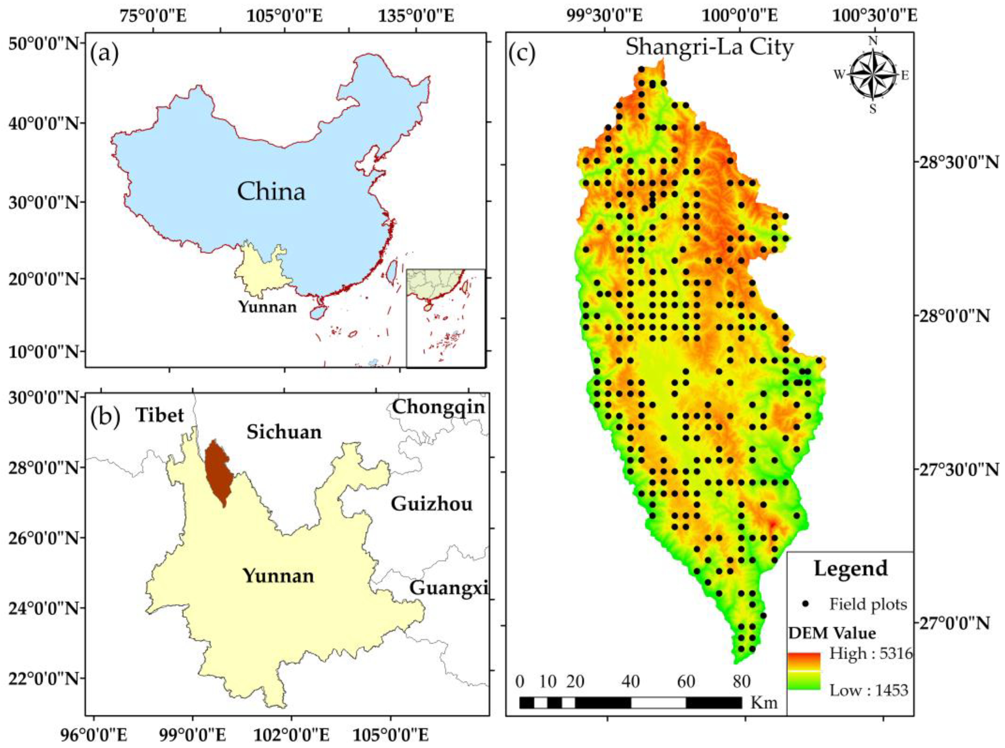
Shangri-La City belongs to the Diqing Tibetan Autonomous Prefecture of Yunnan Province, China, which is located in the hinterland of the Hengduan Mountains on the Qinghai-Tibet Plateau in the northwest of Yunnan Province. The geographic coordinates are between 26°52′11.44″ N and 28°50′59.57″ N, 99°23′6.08″ E, and 100°18′29.15″ E, the total area is 1.142 million ha. The maximum distance from north to south is 218 km, the maximum distance from east to west is 88 km, the average elevation is 3459 m. Shangri-La City belongs to the mountainous cold temperate monsoon climate, resulting in low temperatures throughout the year (the average temperature throughout the year is 5.5 °C), and the alternation of the four seasons is not obvious. In addition, the summer and autumn seasons have more rainfall, while the winter and spring seasons are relatively dry (the average annual precipitation is 617.6 mm). It has intact ecosystems and abundant forest resources, the forest area is 897,500 ha, the forest volume is 139 million m3, and the forest coverage rate is 78.61%. There are mainly 10 types of vegetation; their dominant tree species are Pinus yunnanensis, Pinus densata, Quercus, and Spruce fir. The geographical location of the study area is shown in Figure 1.
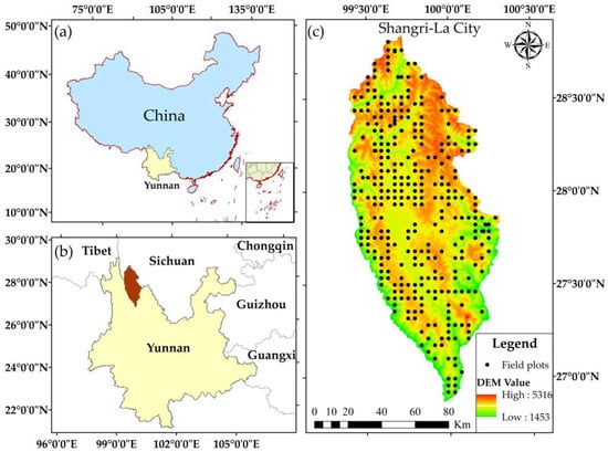
Figure 1.
Location of study area: (a) administrative map of China; (b) the map of Yunnan Province and surrounding provinces, Shangri-la is located in the northwest of Yunnan Province; (c) Shangri-la DEM with spatial resolution of 12.5 m and field plots layout.
2.2. Data and Processing
2.2.1. Data
- Field plots data
In this study, the field plots data we used were the angle gauge controlling sample plots (AGCSP) obtained from the forest management inventory, from the Forestry Department of Yunnan Province; the data were collected by professionals from the forestry department of Yunnan Province in the field according to strict standards in 2016. A total of 323 field plots were used in this study, and they were circular sample plots with a size of 1 ha, including 45 Pinus yunnanensis plots, 87 Pinus densata plots, 138 Spruce fir plots, and 53 Quercus plots. For each plot, the central coordinates, the forest compartment type, the parameters of dominant tree species, the average diameter at breast height (DBH), and the mean tree height were recorded in detail.
- Other data
The auxiliary data include the vector data of the administrative division of Shangri-La City and the forest compartment data of the forest management inventory in 2016. The vector data of the administrative divisions of Shangri-La City is obtained from the geospatial data cloud platform of the Computer Network Information Center of the Chinese Academy of Sciences, it is used for raster data cutting. The forest compartment is the basic unit for forest resource statistics and management, in the forest management inventory, investigators usually use forest compartment surveys to determine the quantity and quality of forests and forest lands to specific plots. The forest compartments provide detailed information on forest lands, including area, land type, forest land type, dominant tree species, and other information. There are the same forest resource attributes in a forest compartment, but there are significant differences in topographic features and environmental and ecological and biological factors among different forest compartments, so the forest compartment was used as a statistical unit to analyze the local spatial variability of four typical forests biomass.
2.2.2. Data Processing
According to forestry industry standards, which include Tree Biomass Models and Related Parameters to Carbon Accounting for Pinus yunnanensis [44], Tree Biomass Models and Related Parameters to Carbon Accounting for Picea asperata [45], Tree Biomass Models and Related Parameters to Carbon Accounting for Abies fabri [46], Tree Biomass Models and Related Parameters to Carbon Accounting for Quercus [47], and biomass model given by Wang et al. [48], we calculated the forest biomass of 323 field plots. The four tree species biomass models are shown in Table 1. Firstly, the biomass of the average tree was calculated according to the average DBH and average tree height of each plot. Secondly, the forest biomass of each plot was calculated according to the number of trees in each plot. Table 2 records the statistical parameters of biomass in 323 plots; Figure 1 shows the spatial distribution of all field plots.

Table 1.
Single-tree biomass model of main tree species selected in Shangri-La City.
Table 2.
Statistical parameters of sample plots biomass.
2.3. Methods
2.3.1. Methods for Estimating Forest Biomass
Geostatistical methods are mostly used in the field of geostatistics, but there are also some applications in the field of forestry. According to the research results of Feng Yimin et al. using a sequential indicator simulation method for simulating forest type distribution [49], this study came up with a geostatistical method for estimating forest biomass. We used the geostatistical variogram as an analysis tool, and the SGCS method based on simple Kriging interpolation to estimate the four typical forests biomass, using the results from the SGCS method as reference data for sampling accuracy analysis and verification. To begin with, the GS+9.0 software is used for conducting variogram analysis based on the biomass data of 323 plots obtained above and performing simple Kriging interpolation according to the analysis results. Moreover, using the forest biomass of plots used for variogram analysis as conditional data [50], determining the optimal number of simulations through multiple attempts. Finally, the biomass of four typical forests in Shangri-La was obtained by SGCS method.
- Variogram
A variogram is a basic tool specific to spatial statistics (also known as geostatistics). Under one-dimensional conditions, it is defined as when the spatial point x changes on the one-dimensional x-axis, the difference of the value Z (x) and Z (x + h) of the regionalized variable Z (x) at points x and x + h, represented as the half of the variance, is called the variogram of the regionalization variable Z (x) in the direction of the x-axis, denoted as γ (x, h). In fact, the theoretical variogram model is unknown, and it is often estimated from valid spatial sampling data. A series of γ2 (h)values can be calculated for various h values. Therefore, a theoretical model is used to fit the values of γ2 (h). Usually, the theoretical model of variogram can be fitted by the spherical model, exponential model Gaussian model, etc., to describe the variation law of regionalized variables. The model of the variogram is uniquely determined by the model type, Sill (C0 + C), Range, and Nugget value (C0) [33,51].
- Sequential Gaussian Conditional Simulation (SGCS)
The SGCS is a spatially stochastic simulation method used to generate spatially explicit estimates of an interest variable based on the theory of regionalized variables and spatial autocorrelation measured by a variogram. Construct a Gaussian function based on known data, and regard each value of the regionalized random variable Z (x) as a random realization of the Gaussian function (that is, the normal distribution function) F(x). At each simulated position x_m, F(x) is derived using the known data Z (x_i) (i = 1, 2, ..., n) and previously simulated values Z (x_j) (j = 1, 2, ..., m − 1) as the conditional cumulative conditional probability density function [52]. The cumulative conditional probability distribution is then utilized to generate the spatial predictions by sequentially stochastic simulation. This method overcomes the smoothing effect disadvantage of Kriging’s estimation and measures the possible values and probabilities of the predicted spatial data at the same time, which can correctly reflect the spatial fluctuation of regional variables and reproduce the fluctuation of the real resource characteristic spatial variation curve [40,41,42,43]. In most cases, the original data do not satisfy the requirements of the simulation process, so it needs to be normalized before being simulated, and finally the inverse transformation method is used to convert the simulation results [53].
2.3.2. Traditional Sampling Methods
Sampling refers to extracting a representative sample from all the samples in this study and estimating the population’s situation based on the sample data, which has the advantages of low costs, fast speed, high precision, and flexibility [11]. The earliest sampling method was purpose sampling, which is an unequal probability sampling method proposed by Norwegian statistician Kangas at the end of the 19th century [54]. The sampling methods used in this study mainly include equidistant sampling (ES) and stratified sampling (SS).
- Equidistant sampling (ES)
Equidistant sampling, also called systematic sampling, means that all the units of the population are arranged in a certain order, the first sample unit is extracted by a simple random method, and then the rest of sample units are sequentially extracted, the samples are distributed according to the determined number of samples and the spacing of sample points. It has the advantages of simplification, uniform distribution, and convenient location [55]. The calculation formula of the sample size and the distance between sample points are as follows [11]:
where n is the sample size, tα is the value of the t statistics from Student’s t-distribution at the significant level α, C is the coefficient of variation, E is the relative error, L is the distance between sample points, and A is the area of the population (It is measured in hectares).
- Stratified sampling (SS)
Stratified sampling, also called type sampling, refers to the random sampling of samples from a population that can be divided into different subpopulations (otherwise known as strata) in a specified proportion from each stratum. After the population is stratified, each stratum is an independent sampling population, random sampling is carried out in each stratum, and there can be no overlap or omission of any units between strata. The advantage of this method is that the sample’s representativeness is better and the sampling error is smaller. Because the sample size allocated to each stratum is different, the proportional distribution method is generally used to allocate the sample size in each stratum; in other words, the number of sample units allocated to each stratum is calculated according to the area proportion (weight) of each stratum [11].
2.3.3. Spatial Sampling Methods and Comparisons with Traditional Approaches
- Spatial sampling based on variation scale
Spatial sampling based on variation scale, it was designed by us considering the spatial autocorrelation of forest biomass. There is a spatial variation scale in objects with spatial autocorrelation, in geostatistics, we used the range to reflect the spatial variation scale of the survey objects. Based on the analysis results of variogram for four typical forests’ biomass, the range was used as the distance between sample points. Then, we calculated the sample size according to the distance between sample points and arrange sample points based on the ES method.
- SS based on local spatial variability
The study area has complex topographic features, and the spatial distribution of forest biomass exhibits significant variability in different local areas. In this context, we designed the SS based on local spatial variability. The sample size was determined according to the population coefficient of variation (CV) from the SGCS results. In addition, the CV chart of four typical forests’ biomass from SGCS results was stratified based on the SS’s theory, and the pixels with similar spatial variation characteristics were grouped together. We used the proportional distribution method to calculate the sample size for each stratum, and arranged the sample points for each stratum based on the ES method.
As a specific representation of the sampling population, the sampling frame should initially be clearly defined in the sampling survey [56]. According to the forest compartment data from the forest management inventory in Shangri-La City in 2016, the distribution range of four typical forests should be extracted as the sampling frame of this sampling design. The sampling frame area is 691,602.3 ha, the sampling unit was a square plot of 100 m × 100 m, and the number of population units was 691,603.
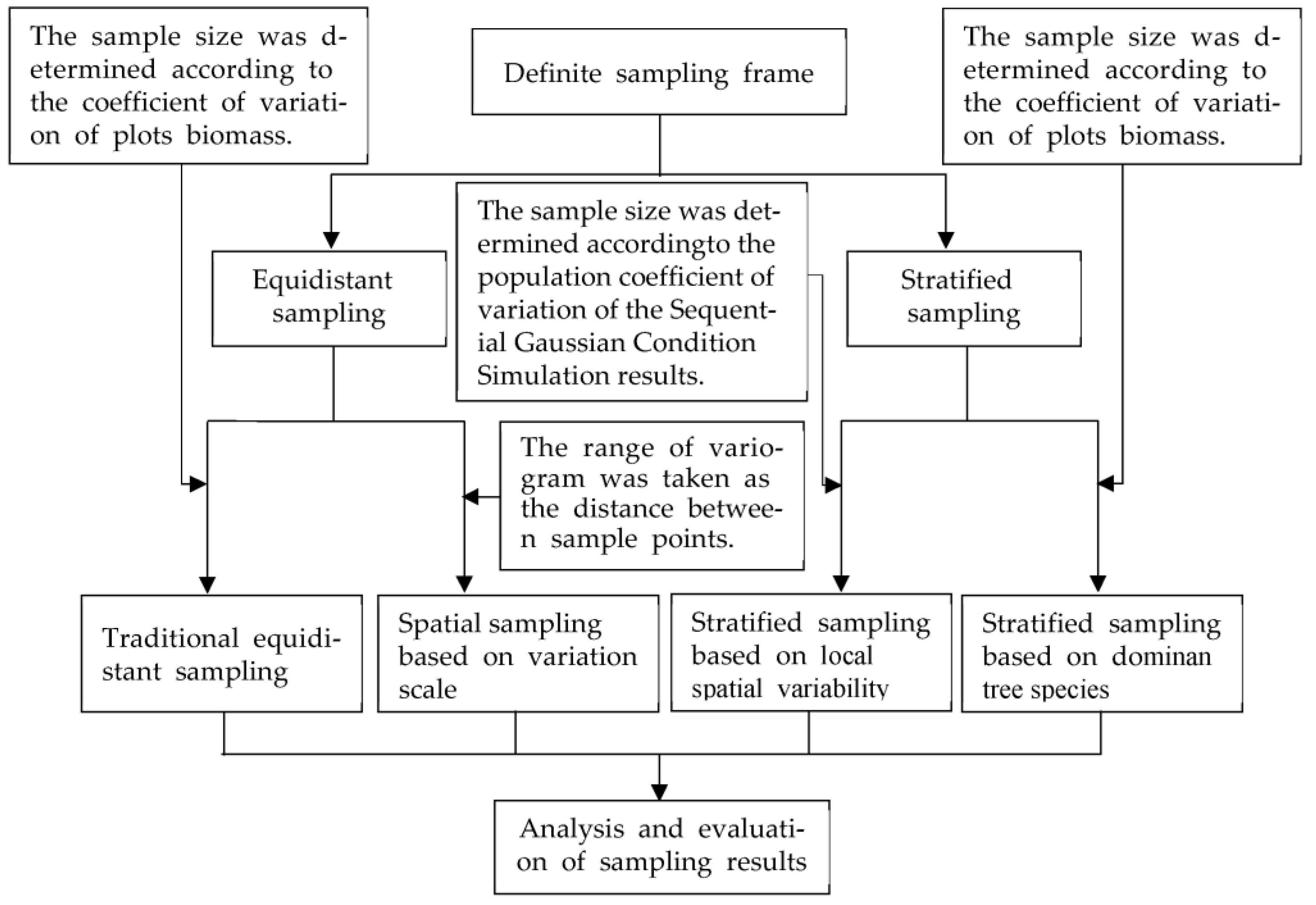
Different sampling methods result in different sample sizes and obtain different sampling accuracy. Considering the differences, advantages, and disadvantages of sampling methods, we used two spatial sampling methods and two traditional sampling methods to conduct a sampling survey on four typical forests’ biomass and conducted a comparative analysis of sampling results. The sampling technical route is shown in Figure 2.
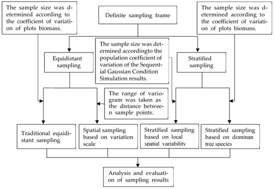
Figure 2.
Sampling technology roadmap.
2.3.4. Accuracy Evaluation
- Forest biomass simulation accuracy
This study used the SGCS method based on the data from 323 biomass field plots to obtain the spatial distribution results of four typical forests’ biomass. Furthermore, we calculated the median of the confidence interval for the total biomass value using the 323 field plots of biomass. The Overall Estimate Consistency (OEC) is determined by the ratio of the total biomass estimated by simulation (TBS) to the median of the confidence interval for the total biomass value calculated by the plots (TBP). The accuracy of the simulation results is evaluated according to the consistency of the OEC [57], and the calculation formula is as follows.
a. Confidence interval:
where is the standard error, S is the standard deviation, n is the number of field plots, is the estimated error limit, is the confidence interval of the overall estimated total value, and a is the field plot area.
b. Overall Estimate Consistency (OEC):
where is the biomass value of the i-th field plot, m is the total number of pixels, and is the simulated value of the j-th pixel. OEC represents the closeness of the simulated population value to the ground sample’s estimated population value, and when the two are equal, OEC = 1.
- Sampling accuracy
According to the biomass value corresponding to the sample points, the sampling accuracy was calculated, we used the relative error and sampling estimation accuracy to analyze, and evaluate each sampling method.
a. ES relative error:
where is the variance of the sampling estimated value, n is the sample size, and is the estimated value of the sampling mean.
b. SS relative error:
where is the estimated mean of the sampling population, l is the number of strata, is the weight of each stratum, is the sample mean of each stratum, is the variance of the population mean estimate, and is the variance of the sampling estimated value of each stratum.
c. Sampling estimation accuracy:
3. Results
3.1. Sequential Gaussian Condition Simulation of Forest Biomass
3.1.1. Variogram Analysis of Forest Biomass
- Normal distribution test of data
In spatial statistics, it is required that the data approximately obey the normal distribution in order to perform SGCS [58]. We used SPSS to test the biomass data structure of the 323 field plots, through the test, it was found that the biomass data did not conform to the normal distribution, so the cubic root transformation was performed on it. The transformed data approximately obeys the normal distribution and satisfies the conditions of spatial statistics, so it can be used to construct a variogram model for subsequent analysis. The histogram of the frequency distribution of biomass data before and after transformation is shown in Figure 3.
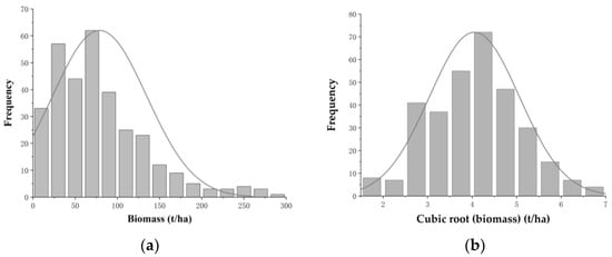
Figure 3.
(a) Histogram of initial forest biomass; and (b) histogram of the transformed forest biomass.
- Variogram analysis of forest biomass
In this study, GS+9 was used to analyze the variogram of forest biomass data from 323 field plots [59]. The spherical model, exponential model, and Gaussian model were utilized to model and predict the variogram of forest biomass, and the models were evaluated using the determination coefficient (R2), the residual sum of squares (RSS). The ratio of the nugget to the sill (C0/(C0 + C)) reflects the spatial variability, it is divided into three grades, 0%–25%, 25%–75%, and more than 75%, which, respectively, indicates that the spatial autocorrelation is strong, moderate, and weak. Generally, the greater the ratio, the greater the spatial variability or the weaker the spatial autocorrelation. A ratio of more than 75% implies that the spatial variability of forest biomass is greatly caused by random changes [33,34]. On the other hand, a ratio of smaller than 75% implies that the spatial autocorrelation is strong due to structural factors. Table 3 shows the results of the variogram structure analysis of forest biomass.
Table 3.
Parameters of forest biomass variograms fitted.
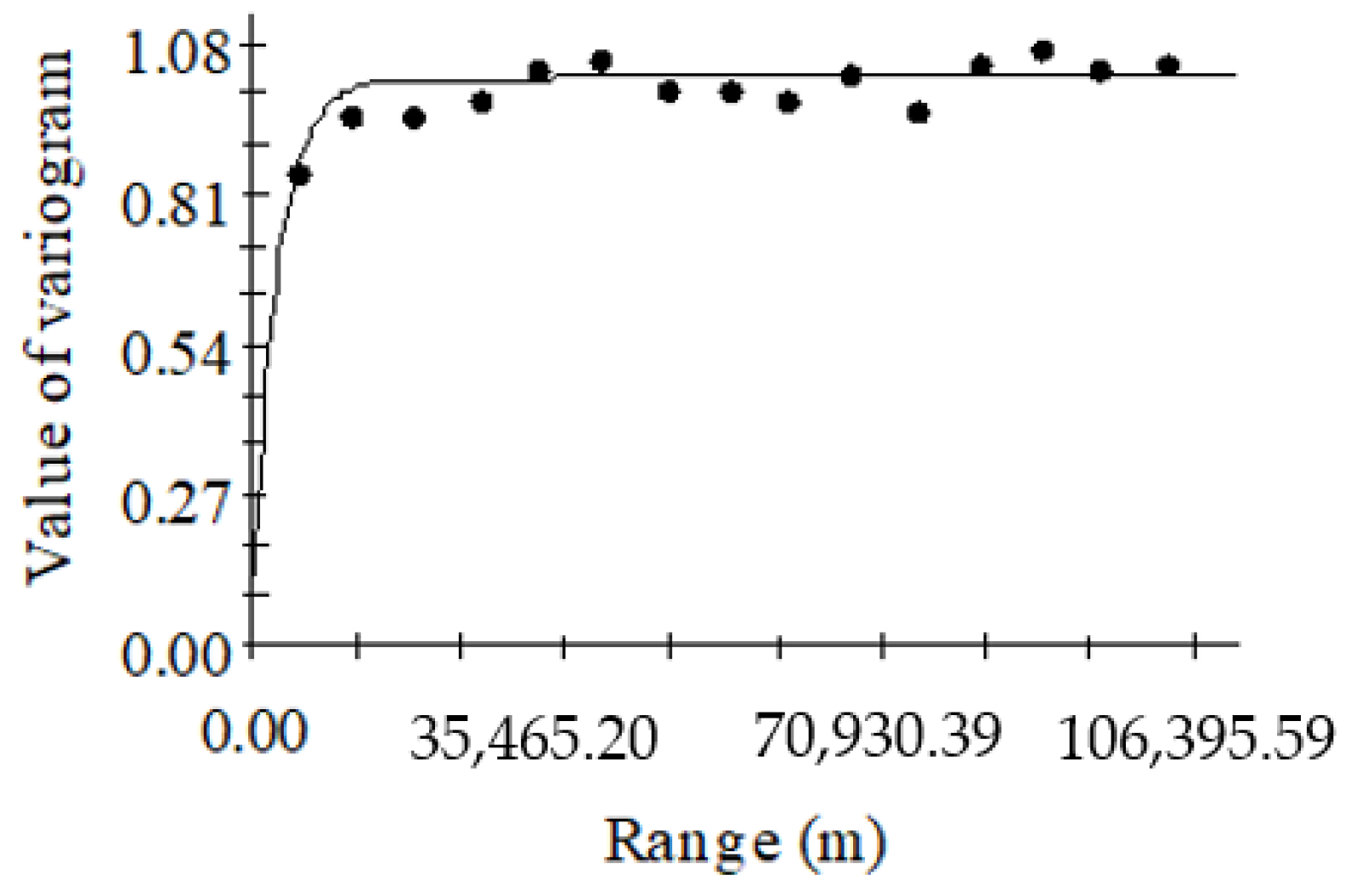
The results of forest biomass variogram analysis showed that the R2 of the exponential model was the highest (R2 = 0.571), and the RSS was the smallest (RSS = 0.0190), so the model fitting effect was the best. The ratio of nugget to sill was 11.67%, indicating that forest biomass has high spatial autocorrelation. The range was 8700 m, indicating that the maximum spatial correlation distance of forest biomass was 8700 m. Within the range, there is spatial correlation; otherwise, there is no spatial correlation [32]. The exponential model formula of forest biomass is shown in Equation (14), and Figure 4 is the variogram fitted by the exponential model.
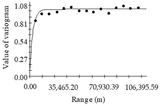
Figure 4.
Variograms diagram of forest biomass.
According to Figure 4, we know that when the range is 0, the value of the variogram is called the nugget value (C0 = 0.119), which represents the amount of random variation [32]. As the range increases, the value of the variogram () gradually increases from the nugget value to a stable state, where the variogram value is called the sill value (C0 + C = 1.02).
3.1.2. Sequential Gaussian Condition Simulation of Forest Biomass
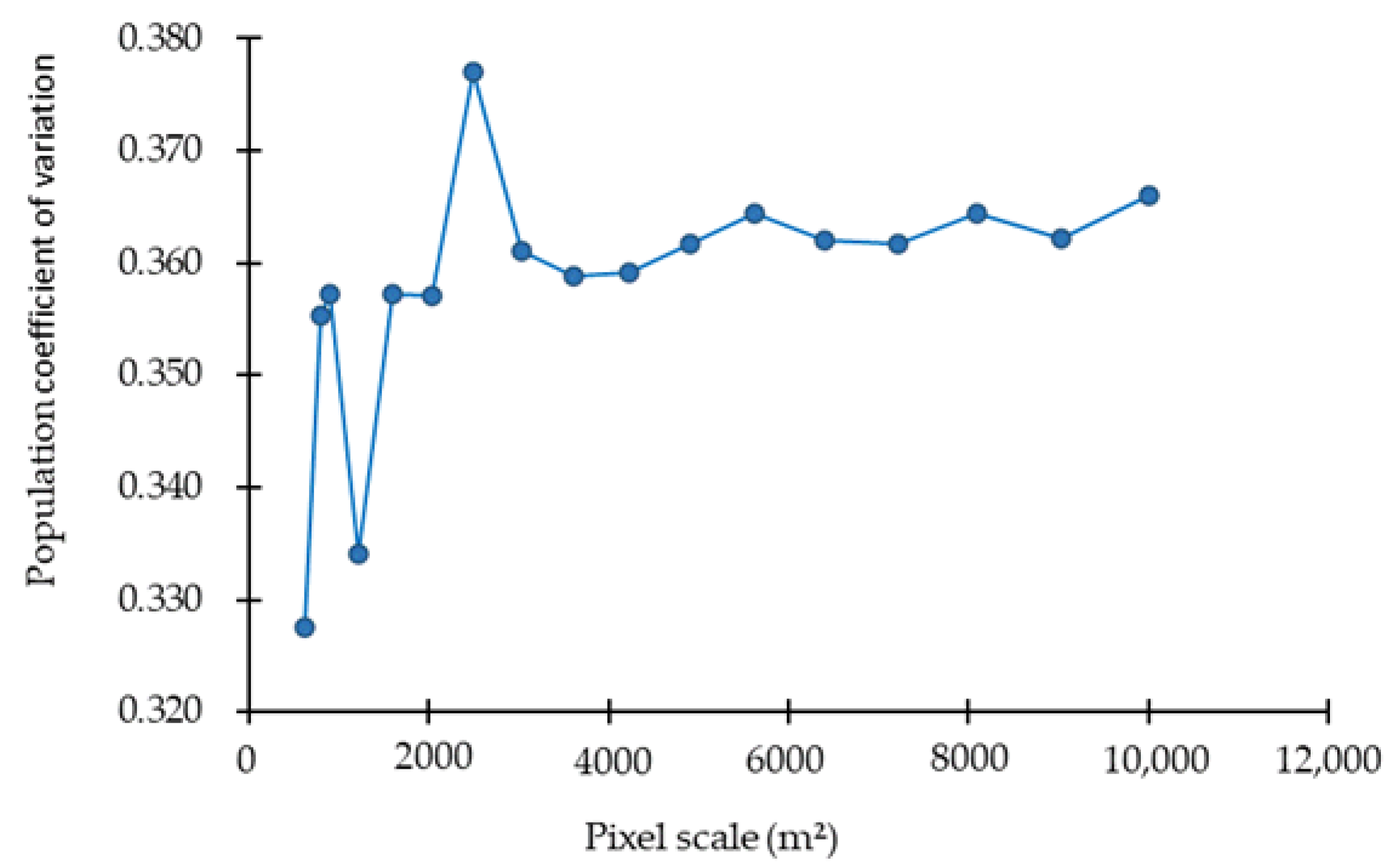
In this study, GS+9 and ArcGIS 10.5 were used to achieve the SGCS of four typical forests’ biomass. Firstly, GS+9 was used to fit the variogram of 323 biomass field plots. Secondly, the parameters of the optimal variogram model (including range, nugget, and sill) are used for simple Kriging interpolation. Finally, the Gaussian Geostatistical Simulations tool in ArcGIS 10.5 was used to achieve the SGCS [60]. Through repeated experiments, we successively set number of SGCS simulations as 10, 25, 50, 75, 100, and 125. The results showed that the variance of the simulated forest biomass values at the pixel level greatly changed as the number of simulations increased and tended to be stable when the number of simulations was 50. Therefore, the number of the SGCS simulations was determined to be 50. In addition, we analyzed the effect of different pixel sizes on the biomass population coefficient of variation (CV). The simulated raster data of different pixel sizes from 25 m × 25 m to 100 m × 100 m with an interval of 5 m were output so as to determine the optimal pixel size. Figure 5 shows the change of the biomass population CV against pixel sizes.

Figure 5.
Population variation coefficient of biomass at different pixel sizes.
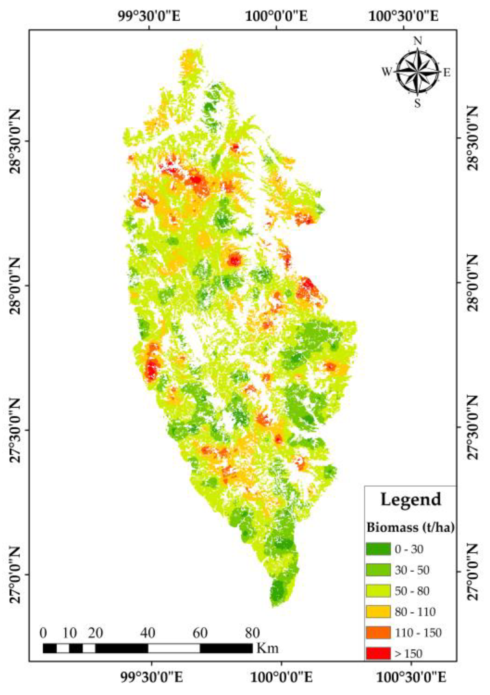
According to the experimental results, we found that the biomass population CV basically tended to be stable when the output pixel area was 3025 m2. In order to match the size of the field plot, the pixel size of SGCS was determined 100 m × 100 m. Since we performed cubic root transformation on the original data, the inverse transformation of simulation results was required after the simulation was completed, and the spatial distribution results of four typical forests biomass were finally obtained, as shown in Figure 6.

Figure 6.
Spatial distribution map of four typical forests’ biomass.
Based on the biomass data of 323 field plots, the median confidence interval of the biomass population value was 54,567,476.7 tons. However, the biomass population value of the four typical forests by using the SGCS method was 47,527,599.6 tons, and it was distributed between 7.1 t/ha and 247.4 t/ha, the average biomass was 69 t/ha. They were close to the biomass data of the Shangri-La forest management inventory in 2016. In addition, the OEC was 0.871, which was closer to 1. Therefore, the four typical forests’ biomass estimation results obtained by the SGCS method satisfied the accuracy requirements and can be used for sampling survey research.
3.2. Analysis of Local Spatial Variability for Four Typical Forests Biomass
As a regionalized variable, forest biomass has different spatial variability from one location to another due to the influence of various habitat factors, which is manifested by the differences in different locations. In order to obtain the spatial variability of the local location of four typical forests’ biomass, we took the forest compartment data of four typical forests in the forest management inventory in Shangri-La in 2016 as the statistical unit and analyzed the spatial variability of forest biomass in each forest compartment according to the spatial distribution results of four typical forests biomass simulated by SGCS.
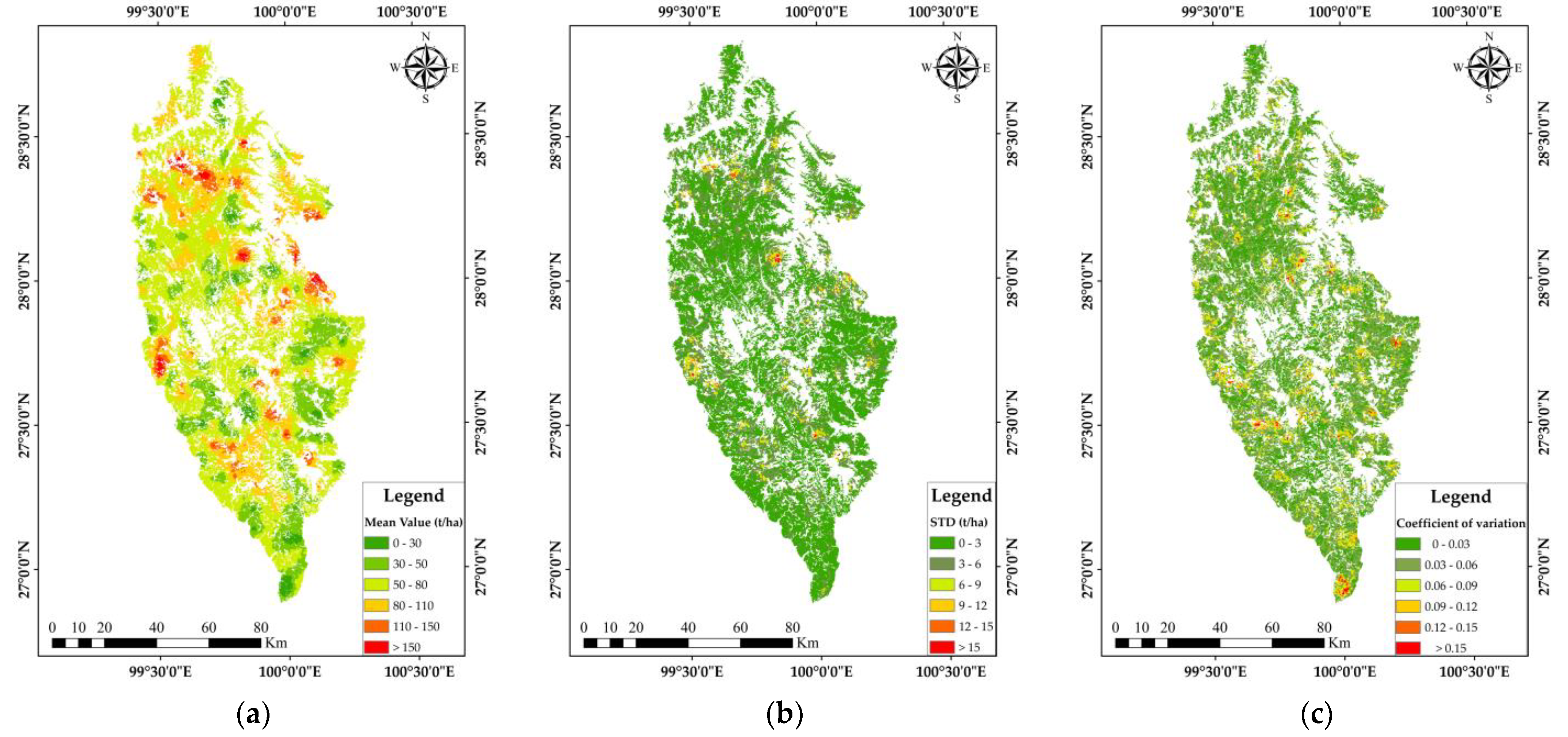
Firstly, according to the results of 50 SGCS runs, the “Zonal Statistics as Table” tool in ArcGIS 10.5 was used to obtain the mean chart and standard deviation (STD) chart of all pixels in each forest compartment. The mean chart provides the mean value of biomass estimates after 50 simulations of all pixels in each forest compartment, and the STD chart shows the variance of biomass estimates in each forest compartment. Then, the ratio calculation between the STD chart and the mean chart was carried out to obtain the CV chart of four typical forests’ biomass in each forest compartment, which reflected the local spatial variation characteristics of forest biomass in each class. The mean value, STD, and CV of biomass of forest compartments are shown in Figure 7.
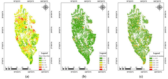
Figure 7.
(a) Mean biomass based on forest compartment data of four typical forest types as statistical units; (b) biomass standard deviation based on forest compartment data of four typical forest types as statistical units; (c) biomass coefficients of variation based on forest compartment data of four typical forest types as statistical units.
According to the CV chart, we can draw some conclusions that the maximum CV of forest biomass was 0.3, the minimum CV was 0, and the CV of forest biomass in most areas of Shangri-La ranges from 0 to 0.12. The CV chart exhibits irregular and fragmented characteristics, which are similar to the spatial structure attributes of forest distribution. The area with a small CV indicates a small change in biomass; on the contrary, it indicates a significant difference in biomass compared to the surrounding area.
3.3. Sampling of Forest Biomass
3.3.1. Equidistant Sampling
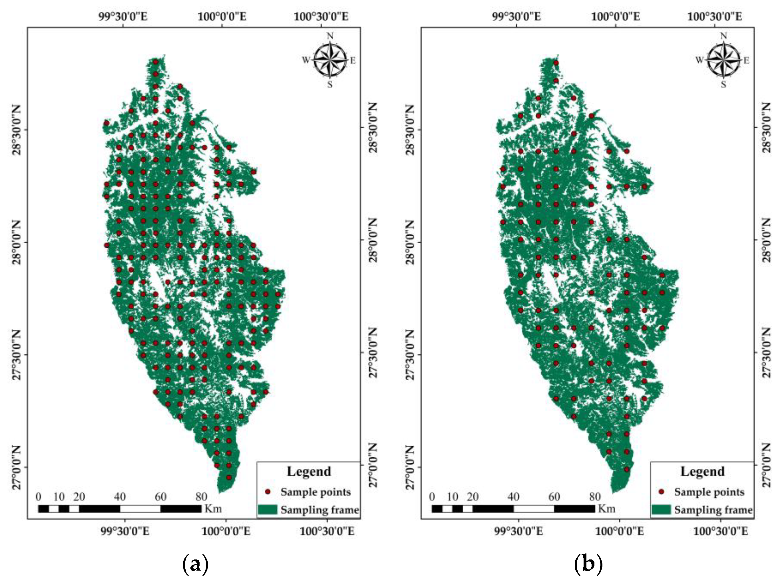
Based on the biomass of 323 field plots, the CV was 0.706. Under the condition of 95% confidence probability, the sampling design accuracy was set to 90%. According to the sample size estimation formula of ES to calculate the sample size, it was 191, and the distance between sample points was 6017 m. Finally, the sampling points are arranged according to the ES method. Based on the results of the variogram analysis of forest biomass, the range (8700 m) of the exponential model was taken as the distance between sample points to design ES, the sample size was 92. We arranged the sampling points according to the distance between the sample points and the sample size. The layout of sample points by two ES methods is shown in Figure 8.

Figure 8.
Comparison of two equidistant sampling methods for sample layout: (a) traditional equidistant sampling methods of sample layout; (b) spatial sampling based on variation scale of sample layout.
3.3.2. Stratified Sampling
- SS based on local spatial variability
Using the forest compartment data of four typical forest types as statistical units, the CV chart obtained by SGCS reflects the local spatial variation of forest biomass. In this study, the CV chart of four typical forests’ biomass was stratified based on the SS’s theory, and the pixels with similar spatial variation characteristics were grouped together. According to the cumulative distribution histogram of pixel values in the CV chart, the Jenks optimal natural fracture method in ArcGIS 10.5 was used to stratify them. According to the breakpoint of the data itself, the cluster analysis was carried out to minimize the intra-class difference and maximize the inter-class difference, and all pixels were divided into three strata. Based on the population mean and STD of biomass simulation results, the CV was 0.366. Under the condition of 95% confidence probability, the sampling design accuracy was set at 90%, and the sample size was 52. The sample size of each stratum is assigned according to the proportion of the total pixel CV of each stratum to the total pixel CV of all pixels. The distance between sample points was calculated according to the sample size allocated and the total area of each stratum, and the sampling points were arranged according to the ES method within each stratum. Table 4 shows the weight and sample size distribution of each stratum and the layout of sample points of each stratum as shown in Figure 9.
Table 4.
Stratified sampling based on local spatial variability weight and sample size distribution.
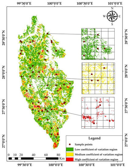
Figure 9.
Layout of stratified sampling points based on local spatial variation.
The result of stratification according to the natural breaks (Jenks) method, the medium CV region has the highest proportion of total CV in the three stratum CV region, accounting for 43.37% of the total value, and the sample size assigned is 23. However, the region with the lowest proportion is the high CV region, accounting for 13.99%, and the sample size assigned is 7.
- SS based on dominant tree species
According to the same sample size as the traditional ES (n = 191), the distribution range of each tree species was divided into one stratum, which was divided into four strata according to the distribution range of the four dominant tree species. The proportional distribution method was adopted to allocate each stratum’s sample size according to the proportion of the area occupied by each stratum, and the distance between sample points within each stratum was calculated, respectively. The sample points were arranged according to the ES method within each stratum. Table 5 shows the area proportion of each stratum, the sample size and the distance between sample points, and the layout of sample points in each stratum as shown in Figure 10.
Table 5.
Stratified sampling based on dominant tree species weight and sample size distribution.
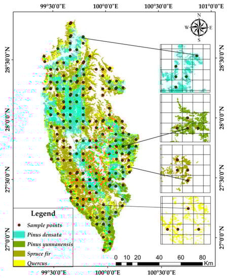
Figure 10.
Layout of stratified sampling points based on dominant tree species.
From the distribution of the four dominant tree species in Figure 10, it can be seen that the Pinus yunnanensis and Spruce fir forests are mainly distributed in the south of Shangri-La. Based on statistical and analytical results, the area of Pinus yunnanensis forests accounted for the smallest proportion of the total area of the four typical forests, accounting for 11.5%, and the allocated sample size was 22. However, the largest proportion of the area is the Spruce fir forest, which accounts for 43.46% of the total area, and the allocated sample size was 83.
3.4. Accuracy Analysis of Sampling Results
3.4.1. Analysis of Variance for Stratified Variables
According to the sample points laid out by the two SS methods and the four typical forest biomass spatial distribution results obtained by the SGCS method, the biomass corresponding to the sample points of each sampling method was extracted, respectively, and the variance of stratified variables of the two SS methods was analyzed, as shown in Table 6.
Table 6.
Results of variance analysis for different stratified variables.
3.4.2. Sampling Accuracy Comparison
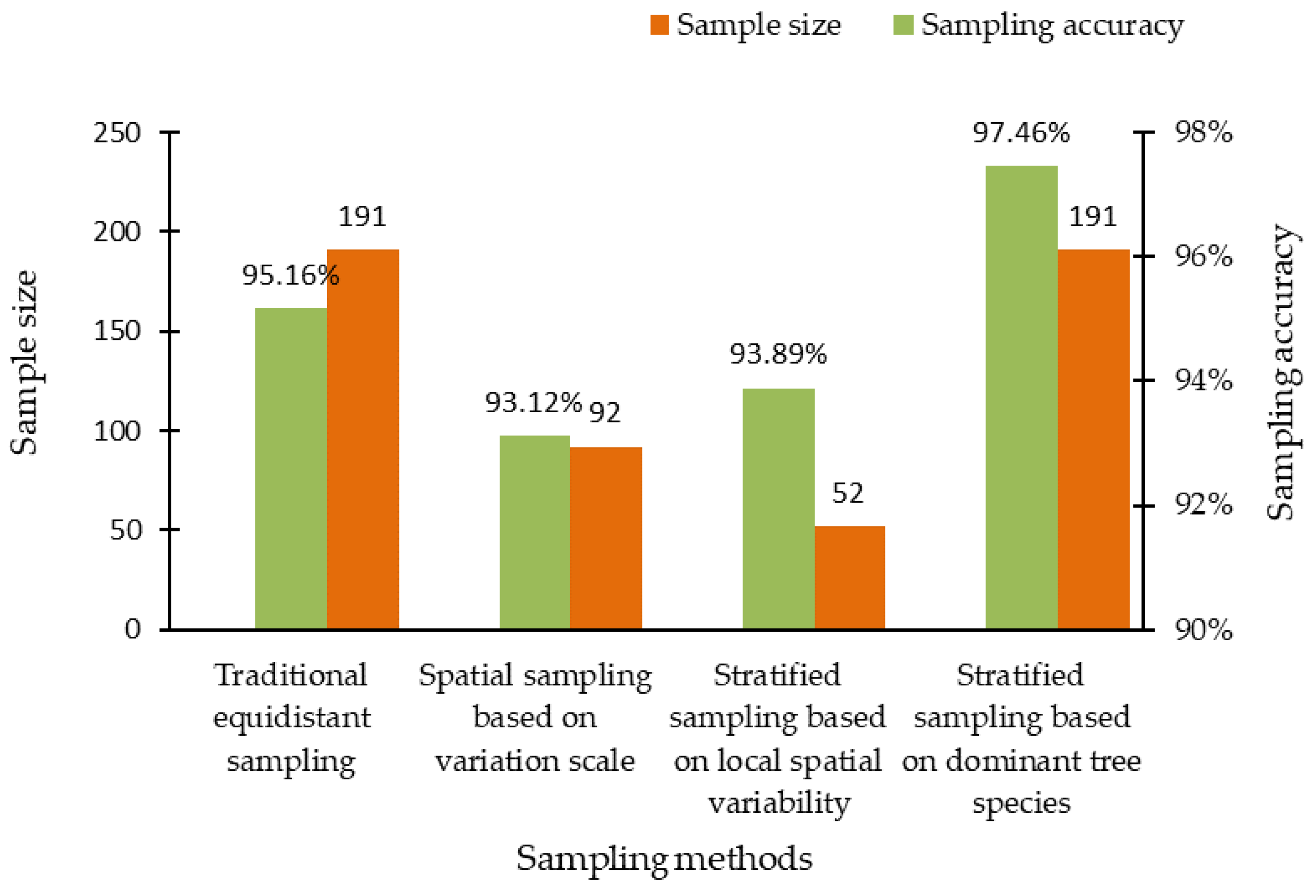
Different sampling methods produce a different effect on sample size and accuracy. Based on the results of the spatial distribution of four typical forests’ biomass obtained by SGCS, the biomass corresponding to the sample points of the four sampling methods was extracted, respectively. We calculated the sampling relative error and accuracy to analyze and evaluate each sampling method. These results showed that the estimation accuracy of the four sampling methods was higher than the design accuracy. On the premise of satisfying the requirements of sampling design accuracy, by comparing the sample size, we can view that the spatial sampling method based on variation scale was better than the traditional ES, and the SS method based on local spatial variability was better than the SS method based on the dominant tree species. Table 7 shows the accuracy analysis results of the four sampling methods. Figure 11 intuitively reflects the sample size and sampling accuracy of the four sampling methods.
Table 7.
Comparative analysis of the results of four sampling methods.

Figure 11.
Comparison of sample size and sampling accuracy among four sampling methods.
Based on the experimental results, we can draw some conclusions that the accuracy of the four sampling methods is higher than that of the sampling design accuracy. Among them, the most accurate sampling method is SS based on dominant tree species. Comparing the two ES methods, although the accuracy of the traditional ES was 2.04% higher than that of the spatial sampling based on the variation scale, the sample size required by the traditional ES was more than twice that of the spatial sampling based on the variation scale. Furthermore, the accuracy of SS based on local spatial variability was reduced by 3.57% compared with SS based on dominant tree species, but the required sample size was far less than that of SS based on dominant tree species. In order to evaluate the four sampling methods more intuitively, we used sampling accuracy divided by sample size to calculate the sample cost-efficiency indicator, leading to the sampling efficiency per unit cost. In the same order as the sampling methods listed in Table 7, the sampling efficiency per unit cost of the four sampling methods is 0.0050, 0.0101, 0.0181, and 0.0051, respectively, the sampling method with the highest sampling efficiency per unit cost is SS based on local spatial variability, and the lowest is traditional ES. Therefore, under the condition of satisfying the sampling design accuracy, the spatial sampling methods have great advantages over the traditional sampling methods.
4. Discussion
The development of classical statistics makes the sampling survey technique widely used in the investigation of forestry resources [5]; ES and SS methods are the research hotspots at present. However, traditional sampling methods have a lot of disadvantages, including high sampling costs, redundant sample information, unrepresentative sample layout, and low sampling efficiency [17,18,19,20]. The emergence of spatial statistics leads many researchers to propose spatial sampling methods. The purpose of this study is to analyze the advantages and practicability of spatial sampling methods. Based on the variogram theory of geostatistics, two spatial sampling methods based on variation scale and local spatial variability are proposed by taking the research cases of four typical forest biomass in Shangri-La City, Yunnan Province, China, so as to solve the problems of redundant sample size and unreasonable layout in traditional sampling methods.
4.1. Application of Geostatistics in Spatial Sampling
The traditional sampling survey of forest resources is based on classical statistics; however, classical statistics believe that randomly distributed sample points are independent of each other. As a natural resource with spatial continuity, forests exhibit significant spatial autocorrelation in their spatial distribution and pattern. The traditional sampling method neglects the spatial correlation of forests and only studies a certain inherent attribute of the forest, without involving the spatial structure characteristics of the surveyed objects, which is not in line with the actual situation of forests. Many researchers have considered the drawbacks of traditional sampling and introduced spatial sampling methods to improve sampling efficiency and accuracy. Therefore, it is necessary to construct an optimization objective function and use optimization solving methods to automatically generate sampling layout optimization plans. Geostatistics is based on the theory of regionalized variables and uses variograms as a unique tool for studying spatial relationships. This method has great advantages in studying natural things that exhibit randomness, structural or spatial correlation, and dependence in spatial distribution. Wang et al. used a variogram to analyze the spatial variability of the research object and estimated the local CV of the coverage factor using the results from the sequence Gaussian co-simulation method. Then, the CV was used to calculate the local sampling distance for spatial and temporal changes. Finally, they designed spatial sampling based on local variability to monitor relevant soil erosion cover factors for an installation in Fort Riley, USA [61]. Anderson et al. used sequential Gaussian co-simulation, combined with remote sensing and ground data to calculate the CV of the pixels to be estimated. They proposed a local variability sampling design method based on ground and vegetation cover factors, which sampled and plotted soil erosion monitoring and vegetation cover coefficients in Fort Hood, Texas, USA [62]. Xiao et al. analyzed the spatial variability of vegetation cover factors, using geostatistical methods to estimate appropriate plot size and sample size, they introduced cost into sampling design from the perspective of measurement time. The research results showed that the impact of plot size on local estimation Kriging standard error is greater than that of sample size, while the impact of sample size on global estimation accuracy is greater than that of plot size [63].
Based on the theory of geostatistics, the issues considered not only include global and local sampling, plot size and sample size, and plot shape, but also the shape of the sampling grid, which directly affects the spatial layout of the sample points and indirectly affects sampling efficiency, costs, and accuracy. Mcbratney et al. calculated the variance of grid spacing and block size range by Kriging interpolation on regular rectangular and triangular grids of the data and previously determined semi-variance maps, and designed sampling plans to monitor soil changes based on different sampling grids. The results indicate that equilateral triangular grids are the best sampling scheme, with an efficiency of approximately 10% higher than square grids [64]. However, if there are different semi-variograms in different parts of the same region, and the differences are significant, then using inconsistent grids and different optimal sampling strategies may be worthwhile [65].
Geostatistics theory plays an important role in spatial sampling. Spatial sampling methods based on geostatistics not only consider the spatial correlation of sampling variables, but also consider the maximum representativeness and redundancy of sample information, which has higher cost-effectiveness compared to traditional sampling methods.
4.2. Spatial Autocorrelation Analysis of Survey Samples
According to the first law of geography proposed by Tobler, all things are interconnected, but the closer things are, the stronger the connection between them. This law indicates that when analyzing spatial objects, it cannot be assumed that the survey samples in the space are unrelated and independent of each other, which contradicts the basic assumptions of most classical statistical sampling analysis [66]. A large number of survey samples are spatially autocorrelated with each other, implying the existence of duplicated information. More precisely, due to the spatial autocorrelation of survey samples, the effective sample size will be smaller than the actual sample size, this is the support of the principle that spatial sampling surveys can reduce costs [67]. Therefore, a key step before conducting spatial sampling is to analyze the spatial autocorrelation of sample variables. Only survey subjects with significant spatial autocorrelation can the use of spatial sampling methods be scientific and feasible [68].
In many studies, researchers generally adopt Moran’s I to analyze the spatial correlation of research objects [69]. With Moran’s I > 0, the survey subjects show a spatial positive autocorrelation, and the correlation increases with the increase in the value; Moran’s I = 0, the survey subjects exhibit spatial randomness, while with Moran’s I < 0, the survey subjects showed a negative spatial autocorrelation, and the correlation weakened as the value increased [70]. We analyzed the spatial autocorrelation of four typical forest biomass by the range of variogram and the ratio of nugget to sill (C0/(C0 + C)), the ratio is divided into three grades, 0%–25%, 25%–75%, and more than 75%, which, respectively, indicate that the spatial autocorrelation is strong, moderate, and weak. Researchers can not only use this method to analyze the spatial autocorrelation of survey objects, but also intuitively see the strength degree of spatial autocorrelation. This application provides an effective spatial autocorrelation analysis method for studying survey objects with spatial correlation, at the same time, it also provides strong technical support for the application of spatial sampling methods in forest resource surveys.
4.3. Sensitivity Analysis of Sampling Intensity for Different Sampling Methods
At present, the popular sampling methods are systematic sampling and SS. However, traditional sampling methods have many drawbacks, as they do not involve the spatial correlation and variability of the sampling objects, resulting in redundant sample information and a lack of representativeness in sample layout and design. Systematic sampling requires a large number of samples to ensure its representativeness for complex populations [16]; SS needs to use scientific methods to select hierarchical variables, which has great limitations [20,21]. In this context, the spatial sampling method can solve the problems existing in traditional sampling methods, as it can take into account the spatial location and distribution of forest resources [71].
The most crucial issue for sampling is the selection of sample points and the determination of sample size, because the sample is representative of the sampling population, and its quantity has a great influence on the sampling accuracy and efficiency [7]. In order to satisfy the accuracy requirements, different sampling methods require different sample sizes. In this study, the sample size of both traditional sampling methods was determined by calculating the biomass CV of 323 field plots with a reliability of 95%, and the sampling accuracy was higher than the initial design accuracy. According to the results of the variation function analysis, we designed a spatial sampling method based on variation scale using variation range as the distance between sample points. The population CV was calculated according to the simulation results of four typical forests’ biomass, so as to determine the sample size required by the SS method based on local spatial variability. The accuracy of both spatial sampling methods is also higher than the design accuracy, but the sample size is largely smaller than that of traditional sampling methods. After comprehensive analysis and comparison, the spatial sampling method outperforms traditional sampling in terms of sampling efficiency and cost.
It was compared with simple Kriging, the spatial distribution results of four typical forests biomass based on SGCS can overcome some smoothing effects [38,39]. Although the accuracy of the simulation results satisfied the requirements, the extreme values in the known data could disappear, and the variance of the estimated data was reduced. Kriging is unable to accurately reflect the spatial variation of forest biomass. For the SS based on local spatial variability, we obtained a sample size that is relatively small, although the uncertainty of the simulation quantity and the output pixel size were analyzed and compared, and the sampling accuracy satisfied the requirements. The distribution of the four typical forests is very extensive, and if the sample size is small, there may be limitations in representativeness, so the sample size of this sampling method still needs to be optimized.
4.4. Determination of Stratified Variables in Stratified Sampling
The SS method can select and determine samples more scientifically to reduce sampling error and improve sampling efficiency, but if the stratified technology is not reasonable, the sampling precision will also be reduced [20,21]. Therefore, the key of SS is to determine the stratified variables, which must well represent the attributes and characteristics of the respondents. Stehman et al. analyzed the overall coverage change of the subtropical forest biome based on MODIS data from 2000 to 2005 and designed SS according to different coverage change degrees [15]. Lewis Jack proposed a model-based sampling method that optimizes stratum and sample allocation through regression or ratio estimator [72]. Considering the local spatial variability of the survey objects, we propose a new spatial SS method. Spatial stratification refers to dividing the overall unit into several types or layers based on its attribute characteristics and spatial continuity [23]. In traditional SS, the sample points have no spatial coordinate information, which leads to the stratified results being spatially discrete. According to Tobler’s first law, objects that are closer together are more similar [66]. If the traditional SS method is used, objects on the same layer may be far apart in space.
Traditional SS of forest resources uses land use types, forest types, tree species, forest age, and other attributes as stratified variables [16,73], higher sampling accuracy can be obtained, which is also analyzed in this study. We took the forest compartment data of four typical forests as statistical units to obtain the mean chart, STD chart, and CV chart of forest biomass in each forest compartment. Jenks’ best natural fracture method in ArcGIS 10.5 was used to stratify the CV chart and as stratified variables to design SS based on local spatial variability. When analyzing local spatial variability, we used forest compartment data covering four typical forest distributions in the study area as the minimum unit; therefore, from the perspective of spatial continuity of stratified variables, the spatial stratification method is reasonable, which is also an innovation of this study. Furthermore, the number of strata also has an impact on the sample size and accuracy, Wang et al.’s research shows that when the study area was partitioned into three strata, the number of sample plots obtained with the same accuracy is less than the number of sample plots obtained without strata and with two strata [74]. In this study, we only divided the biomass CV into three strata, and in future studies, we can try to divide the CV into different numbers of strata to achieve higher sampling accuracy.
5. Conclusions
In this study, we utilized the variogram tool of geostatistics and the SGCS method to achieve the transition of biomass of four typical forests in Shangri-La from point scale to polygon scale, providing a new opportunity and method for the application of geostatistics in large-scale forest biomass estimation. Through the analysis of the variogram of forest biomass, we found that the exponential model can provide the best-fitting effect. The range of the exponential model reflects the maximum spatial influence range of four typical forest biomass, using the range as the sampling grid distance to design spatial sampling can effectively solve the issue of sample redundancy. Shangri-La has complex topographic features and different forest compartments have significant differences in the quantity and quality of forest resources, and environmental, ecological, and biological factors. We used the forest compartment as the smallest statistical unit to analyze the local spatial variability of forest biomass, the spatial distribution characteristics of forest vegetation were fully considered in Shangri-La. According to the results of local spatial variability analysis, we used biomass CV for stratification and designed an SS based on local spatial variability. This spatial SS method not only takes into account the spatial location and distribution of forest biomass, but also makes the distribution of sample points representative. In addition, we introduced a sample cost-efficiency indicator to evaluate spatial sampling methods and traditional sampling methods. The result shows that the sampling efficiency per unit cost of both spatial sampling methods is higher than that of traditional sampling methods, as spatial sampling methods have significant advantages in sample size. Compared to traditional sampling methods, the spatial sampling methods proposed by us effectively optimized the sample size and layout of remote sensing monitoring of forest biomass in Shangri-La. Therefore, under the condition of satisfying the sampling design accuracy, spatial sampling methods greatly reduce sampling costs and improve sampling efficiency.
Sampling is an effective and scientific statistical method that is not only applied in the field of forestry research, but also has some applications in other research fields. Spatial sampling mainly serves to survey objects with spatial correlation and variability. This method has obvious practicality for areas with complex topographic features, such as Shangri-La. Our research results provide a scientific sampling method for investigating forest resources and provide a new research direction for sampling natural resources with obvious spatial correlation and distribution characteristics.
Author Contributions
Conceptualization, S.L. and Q.S.; methodology, S.L., J.Y., Z.Y. and W.Z.; formal analysis, S.L. and Q.S.; resources, Q.S.; writing—original draft preparation, S.L.; writing—review and editing, S.L., L.X., Y.G., S.W. and Q.S.; visualization, S.L. and C.G.; supervision, J.X. All authors have read and agreed to the published version of the manuscript.
Funding
This research was funded by the Joint Agricultural Project of Yunnan Province (Nos. 202301BD070001-002).
Data Availability Statement
The data required for this study can be shared the appropriate authors according to the actual situation.
Acknowledgments
We appreciate the resources provided by our instructors and the efforts of all the authors. Finally, we sincerely thank the editors and reviewers for their valuable comments.
Conflicts of Interest
The authors declare no conflict of interest.
References
- Herold, M.; Carter, S.; Avitabile, V.; Espejo, A.B.; Jonckheere, I.; Lucas, R.; McRoberts, R.E.; Næsset, E.; Nightingale, J.; Petersen, R.; et al. The Role and Need for Space-Based Forest Biomass-Related Measurements in Environmental Management and Policy. Surv. Geophys. 2019, 40, 757–778. [Google Scholar]
- Lisboa, S.N.; Guedes, B.S.; Ribeiro, N.; Sitoe, A. Biomass Allometric Equation and Expansion Factor for a Mountain Moist Evergreen Forest in Mozambique. Carbon Balance Manag. 2018, 13, 23. [Google Scholar] [CrossRef] [PubMed]
- Parresol, B.R. Assessing Tree and Stand Biomass: A Review with Examples and Critica1 Comparisons. For. Sci. 1999, 45, 573–593. [Google Scholar]
- Li, D.; Wang, C.; Hu, Y.; Liu, S. General Review on Remote Sensing-Based Biomass Estimation. Geomat. Inf. Sci. Wuhan Univ. 2012, 37, 631–635. (In Chinese) [Google Scholar]
- Scott, C.T. Sampling Methods for Estimating Change in Forest Resources. Ecol. Appl. 1998, 8, 228–233. [Google Scholar] [CrossRef]
- Rafael, M.N.C.; Eduardo, G.F.; Jorge, G.G.; Carlos, J.C.R.; Rocío, H.C. Impact of Plot Size and Model Selection on Forest Biomass Estimation Using Airborne LiDAR: A Case Study of Pine Plantations in Southern Spain. J. For. Sci. 2017, 63, 88–97. [Google Scholar]
- Nelson, R.; Gobakken, T.; Næsset, E.; Gregoire, T.G.; Ståhl, G.; Holm, S.; Flewelling, J. Lidar Sampling: Using an Airborne Profiler to Estimate Forest Biomass in Hedmark County, Norway. Remote Sens. Environ. 2012, 123, 563–578. [Google Scholar] [CrossRef]
- ÖZÇELİK, R.; Eraslan, T. Two-stage Sampling to Estimate Individual Tree Biomass. Turk. J. Agric. For. 2012, 36, 389–398. [Google Scholar] [CrossRef]
- Wang, Y.; Ni, W.; Sun, G.; Chi, H.; Zhang, Z.; Guo, Z. Slope-adaptive Waveform Metrics of Large Footprint LiDAR for Estimation of Forest Aboveground Biomass. Remote Sens. Environ. 2019, 224, 386–400. [Google Scholar]
- Keller, M.; Palace, M.; Hurtt, G. Biomass Estimation in the Tapajos National Forest, Brazil: Examination of Sampling and Allometric Uncertainties. For. Ecol. Manag. 2001, 154, 371–382. [Google Scholar]
- Song, X.M.; Li, J.L. Sampling Techniques, 2nd ed.; China Forestry Publishing House: Beijing, China, 2007. (In Chinese) [Google Scholar]
- Talvitie, M.; Leino, O.; Holopainen, M. Inventory of Sparse Forest Populations Using Adaptive Cluster Sampling. Silva Fenn. 2005, 40, 101–108. [Google Scholar] [CrossRef]
- Fu, Y.; Lei, Y.; Zeng, W. Uncertainty Assessment in Regional-Scale Above Ground Biomass Estimation of Chinese Fir. Sci. Silvae Sin. 2014, 50, 79–86. (In Chinese) [Google Scholar]
- Yim, J.S.; Kleinn, C.; Kim, S.H.; Jeong, J.H.; Shin, M.Y. A Comparison of Systematic Sampling Designs for Forest Inventory. J. Korean For. Soc. 2009, 98, 133–141. [Google Scholar]
- Stehman, S.V.; Hansen, M.C.; Broich, M.; Potapov, P.V. Adapting a Global Stratified Random Sample for Regional Estimation of Forest Cover Change Derived from Satellite Imagery. Remote Sens. Environ. 2010, 115, 650–658. [Google Scholar] [CrossRef]
- Wang, R.; Yang, Q.; Ou, G.; Xu, H. Forest Biomass Investigation Design Using Stratified Sampling in Simao District. For. Resour. Manag. 2021, 1, 197–202. (In Chinese) [Google Scholar]
- Sullivan, M.J.P.; Lewis, S.L.; Hubau, W.; Qie, L.; Baker, T.R.; Banin, L.F.; Chave, J.; Cuni-Sanchez, A.; Feldpausch, T.R.; Lopez-Gonzalez, G.; et al. Field Methods for Sampling Tree Height for Tropical Forest Biomass Estimation. Methods Ecol. Evol. 2018, 9, 1179–1186. [Google Scholar] [CrossRef] [PubMed]
- Meng, F.M.; Xu, S.C.; Yang, X.M. The Application of Random Sampling Survey Method in the Survey of Non-Productive Consumption of Forest Resources. For. Resour. Manag. 1995, 4, 35–37. (In Chinese) [Google Scholar] [CrossRef]
- Jin, L.W.; Zhao, R.H. A Simple Random Sampling Method for Determining the Optimal Quadrat Size of Dendrolimus Tabulaeformis Pupae. Liaoning For. Sci. Technol. 2001, 2, 42–44. (In Chinese) [Google Scholar]
- Pang, E.; Xu, L.; Zhang, M.; Xu, H. Application of Stratified Sampling of DN Value in Remote Sensing Estimation of Urban Forest Biomass. J. Southwest For. Univ. 2018, 38, 132–138. (In Chinese) [Google Scholar]
- Dillabaugh, K.A.; King, D.J. Riparian Marshland Composition and Biomass Mapping Using Ikonos Imagery. Can. J. Remote Sens. 2008, 34, 143–158. [Google Scholar] [CrossRef]
- Silvio, M.; Federica, L.; Antonio, R.; Gentile, F.F. Cost-effective Spatial Sampling Designs for Field Surveys of Species Distribution. Biodivers. Conserv. 2019, 28, 2891–2908. [Google Scholar]
- Zhang, X.W.; She, G.H.; Wen, X.R.; Lin, G.; Cao, L.; Luo, Y. The Application of Spatial Stratified Sampling in Remote Sensing Monitoring of Forest Cover. J. Nanjing For. Univ. 2012, 36, 81–84. (In Chinese) [Google Scholar]
- Xu, Y.; Li, M.; Hao, S. GIS-Based Sampling Method of Urban Forest Biomass. For. Resour. Manag. 2018, 5, 123–127. (In Chinese) [Google Scholar]
- Gilbert, B.; Lowell, K. Forest Attributes and Spatial Autocorrelation and Interpolation: Effects of Alternative Sampling Schemata in the Boreal Forest. Landsc. Urban Plan 1997, 37, 235–244. [Google Scholar] [CrossRef]
- Matheron, G. Principles of Geostatistics. Econ. Geol. 1963, 58, 1246–1266. [Google Scholar] [CrossRef]
- Hock, B.K.; Payn, T.W.; Shirley, J.W. Using a Geographic Information System and Geostaticstics to Estimate Site Index of Pinus Radiata for Kaingaroa Forest. N. Z. J. For. Sci. 1993, 23, 264–277. [Google Scholar]
- Stark, K.E.; Arsenault, A.; Bradfield, G.E. Variation in Soil Seed Bank Species Composition of a Dry Coniferous Forest: Spatial Scale and Sampling Considerations. Plant Ecol. 2008, 197, 173–181. [Google Scholar] [CrossRef]
- Lark, R.M. Optimized Spatial Sampling of Soil for Estimation of The Variogram by Maximum Likelihood. Geoderma 2002, 105, 49–80. [Google Scholar] [CrossRef]
- Dessard, H.; Bar-Hen, A. Experimental Design for Spatial Sampling Applied to the Study of Tropical Forest Regeneration. Can. J. For. Res. 2005, 35, 1149–1155. [Google Scholar] [CrossRef]
- Samra, J.S.; Gill, H.S.; Bhatia, V.K. Spatial Stochastic Modeling of Growth and Forest Resource Evaluation. For. Sci. 1989, 35, 663–676. [Google Scholar]
- Wang, Z.Q. Geostatistics and Its Applications in Ecology; Science Press: Beijing, China, 1999. (In Chinese) [Google Scholar]
- Ping, Y.; Hua, P.; Yan, L.; Lin, K. Spatial Variability of Soil Physical Properties Based on GIS and Geo-Statistical Methods in the Red Beds of the Nanxiong Basin, China. Pol. J. Environ. Stud. 2019, 28, 2961–2972. [Google Scholar]
- Sahu, B.; Ghosh, A.K.; Seema. Deterministic and Geostatistical Models for Predicting Soil Organic Carbon in A 60 Ha Farm on Inceptisol in Varanasi, India. Geoderma Reg. 2021, 26, e00413. [Google Scholar] [CrossRef]
- Shu, Y.J. Study of Optimization Algorithm about Spherical Model of Semi-Variogram in Geostatistics. Master’s Thesis, East China Institute of Technology, Nanchang, China, 2012. (In Chinese). [Google Scholar]
- Matheron, G. Les Variables Régionalisées et Leur Estimation; Masson: Paris, France, 1965. [Google Scholar]
- Matheron, G. The Theory of Regionalized Variables and Its Applications; Ecole de Mines: Paris, France, 1971. [Google Scholar]
- Facchinelli, A.; Sacchi, E.; Mallen, L. Multivariate Statistical and GIS-Based Approach to Identify Heavy Metal Sources in Soils. Environ. Pollut. 2001, 114, 313–324. [Google Scholar] [CrossRef]
- Zhang, S.; Shao, M.; Li, D. Prediction of Soil Moisture Scarcity Using Sequential Gaussian Simulation in an Arid Region of China. Geoderma 2017, 295, 119–128. [Google Scholar] [CrossRef]
- Qu, M.; Li, W.; Zhang, C. Spatial Distribution and Uncertainty Assessment of Potential Ecological Risks of Heavy Metals in Soil Using Sequential Gaussian Simulation. Hum. Ecol. Risk Assess. 2014, 20, 764–778. [Google Scholar] [CrossRef]
- Zhao, Y.; Shi, X.; Yu, D.; Wang, H.; Sun, W. Uncertainty Assessment of Spatial Patterns of Soil Organic Carbon Density Using Sequential Indicator Simulation, A Case Study of Hebei Province, China. Chemosphere 2005, 59, 1527–1535. [Google Scholar] [CrossRef]
- Juang, K.W.; Chen, Y.S.; Lee, D.Y. Using Sequential Indicator Simulation to Assess the Uncertainty of Delineating Heavy Metal Contaminated Soils. Environ. Pollut. 2004, 127, 229–238. [Google Scholar] [CrossRef] [PubMed]
- Huang, J.H.; Liu, W.C.; Zeng, G.M.; Li, F.; Huang, X.L.; Gu, Y.L.; Shi, L.X.; Shi, Y.H.; Wan, J. An Exploration of Spatial Human Health Risk Assessment of Soil Toxic Metals Under Different Land Uses Using Sequential Indicator Simulation. Ecotoxicol. Environ. Saf. 2016, 129, 199–209. [Google Scholar] [CrossRef] [PubMed]
- State Forestry Administration of China (SFAC). Tree Biomass Models and Related Parameters to Carbon Accounting for Pinus yunnanensis; State Forestry Administration: Beijing, China, 2014. (In Chinese) [Google Scholar]
- State Forestry Administration of China (SFAC). Tree Biomass Models and Related Parameters to Carbon Accounting for Picea asperata; State Forestry Administration: Beijing, China, 2016. (In Chinese) [Google Scholar]
- State Forestry Administration of China (SFAC). Tree Biomass Models and Related Parameters to Carbon Accounting for Abies fabri; State Forestry Administration: Beijing, China, 2016. (In Chinese) [Google Scholar]
- State Forestry Administration of China (SFAC). Tree Biomass Models and Related Parameters to Carbon Accounting for Quercus; State Forestry Administration: Beijing, China, 2016. (In Chinese) [Google Scholar]
- Wang, J.X.; Tang, W.J. Estimation and Analysis of Above-ground Biomass and Carbon Storage of Forest Based on Forest Resource Planning and Design Survey Data: A Case Study of Shangri-La City. J. Green Sci. Technol. 2021, 23, 14–16. (In Chinese) [Google Scholar]
- Feng, Y.M.; Tang, S.Z.; Li, Z.Y. Simulation of spatial distribution pattern of forest types by using sequential indicator simulation. Acta Ecol. Sin. 2004, 24, 946–952. (In Chinese) [Google Scholar]
- Zhao, Y.F.; Sun, Z.Y.; Chen, J. Analysis and Comparison in Arithmetic for Kriging Interpolation and Sequential Gaussian Conditional Simulation. J. Geo-Inf. Sci. 2010, 12, 767–776. (In Chinese) [Google Scholar] [CrossRef]
- Wang, M.; Fan, C.; Gao, B.; Ren, Z.; Li, F. A Spatial Random Forest Interpolation Method with Semi-variogram. Chin. J. Eco-Agric. 2022, 30, 451–457. (In Chinese) [Google Scholar]
- Zhao, Y.; Hua, Q.; Chen, J. Comparison of Kriging Interpolation with Conditional Sequential Gaussian Simulation in Principles and Case Analysis of Their Application in Study on Soil Spatial Variation. Acta Pedol. Sin. 2011, 48, 856–862. (In Chinese) [Google Scholar]
- Lü, X.G.; Wang, D.F.; Jiang, H.F. Reservoir Geological Model and Stochastic Modeling Technique. Pet. Geol. Oilfieid Dev. Daqin 2000, 19, 10–16. (In Chinese) [Google Scholar]
- Kangas, A.; Maltamo, M. Forest Inventory-Methodology and Applications; Springer: New York, NY, USA, 2006. [Google Scholar]
- Yang, G.J.; Yin, J.; Meng, J.; Wang, W.Z. Applied Sampling Techniques, 2nd ed.; China Statistics Press: Beijing, China, 2020. (In Chinese) [Google Scholar]
- Sun, H.H. Application Research of Spatial Stratified Sampling in Forest-Covered Monitoring. Master’s Thesis, Nanjing Forestry University, Nanjing, China, 2013. (In Chinese). [Google Scholar]
- Zhang, M.; Wang, G.; Ge, H.; Xu, L. Estimation of Forest Carbon Distribution for Xianju County Based on Spatial Simulation. Sci. Silvae Sin. 2014, 50, 13–22. (In Chinese) [Google Scholar]
- Shen, G.; Zhang, M. Multi-Scale Regional Forest Carbon Density Estimation Based on Sequential Gaussian Co-Simulation. J. Southwest For. Univ. 2015, 35, 55–62. (In Chinese) [Google Scholar] [CrossRef]
- Akhavan, R.; Amiri, G.H.; Zobeiri, M. Spatial Variability of Forest Growing Stock Using Geostatistics in the Caspian region of Iran. Casp. J. Environ. Sci. 2010, 8, 43–53. [Google Scholar]
- Xu, C.X.; Pu, L.J.; Zhu, M.; Xu, C.Y.; Zhang, M.; Xu, Y. Prediction of Soil Heavy Metals Content Based on Sequential Gaussian Simulation and Evaluation of Its Uncertainties: A Case Study of Soil Hg Content in Yixing. Acta Pedol. Sin. 2018, 55, 999–1006. [Google Scholar]
- Wang, G.; Gertner, G.; Anderson, A.B.; Howard, H. Repeated measurements on permanent plots using local variability sampling for monitoring soil cover. Catena 2008, 73, 75–88. [Google Scholar] [CrossRef]
- Anderson, A.B.; Wang, G.; Gertner, G. Local variability based sampling for mapping a soil erosion cover factor by co-simulation with Landsat TM images. Int. J. Remote Sens. 2006, 27, 2423–2447. [Google Scholar] [CrossRef]
- Xiao, X.; Gertner, G.; Wang, G.; Anderson, A.B. Optimal sampling scheme for estimation landscape mapping of vegetation cover. Landsc. Ecol. 2005, 20, 375–387. [Google Scholar] [CrossRef]
- McBratney, A.B.; Webster, R. The design of optimal sampling schemes for local estimation and mapping of regionalized variables—II: Program and examples. Comput. Geosci. 1981, 7, 335–365. [Google Scholar] [CrossRef]
- McBratney, A.B.; Webster, R.; Burgess, T.M. The design of optimal sampling schemes for local estimation and mapping of regionalized variables—I: Theory and method. Comput. Geosci. 1981, 7, 331–334. [Google Scholar] [CrossRef]
- Tobler, W.R. A computer movie simulating urban growth in the Detroit region. Econ. Geogr. 1970, 46, 234–240. [Google Scholar] [CrossRef]
- Rogerson, P.A. Statistical Methods for Geographical; Sage Publications: London, UK, 2001. [Google Scholar]
- Zhang, X.W. Spatial Sampling Technology and Its Application in Remote Sensing Monitoring of Forest Cover Area. Master’s Thesis, Nanjing Forestry University, Nanjing, China, 2011. (In Chinese). [Google Scholar]
- Wong, D.W.S.; Lee, J. Statistics Analysis of Geographic Information with ArcView GIS and ArcGIS; John Wiley & Sons: Hoboken, NJ, USA, 2005. [Google Scholar]
- Chen, K. Accuracy Assessment Methods Based on Spatial Sampling for Remote Sensing Classification. Master’s Thesis, Shanghai Ocean University, Shanghai, China, 2016. (In Chinese). [Google Scholar]
- Wu, H.; Xu, H.; Tian, X.L.; Zhang, W.F.; Lu, C. Multistage Sampling and Optimization for Forest Volume Inventory Based on Spatial Autocorrelation Analysis. Forests 2023, 14, 250. [Google Scholar] [CrossRef]
- Lewis, J. Stemflow estimation in a redwood forest using model-based stratified random sampling. Environmetrics 2003, 14, 559–571. [Google Scholar] [CrossRef]
- Zhang, C. Forest Carbon Estimation in Three Gorges Region. Ph.D. Thesis, Beijing Forestry University, Beijing, China, 2016. (In Chinese). [Google Scholar]
- Wang, G.; Gertner, G.; Anderson, A.B. Sampling and mapping a soil erosion cover factor by integrating stratification, model updating and Cokriging with images. Environ. Manag. 2007, 39, 84–97. [Google Scholar] [CrossRef]


Disclaimer/Publisher’s Note: The statements, opinions and data contained in all publications are solely those of the individual author(s) and contributor(s) and not of MDPI and/or the editor(s). MDPI and/or the editor(s) disclaim responsibility for any injury to people or property resulting from any ideas, methods, instructions or products referred to in the content. |
© 2023 by the authors. Licensee MDPI, Basel, Switzerland. This article is an open access article distributed under the terms and conditions of the Creative Commons Attribution (CC BY) license (https://creativecommons.org/licenses/by/4.0/).