Global Wildfire Danger Predictions Based on Deep Learning Taking into Account Static and Dynamic Variables

Abstract

Climate change will intensify the danger of wildfires, significantly impacting human life. Deep Learning (DL) has been extensively applied in wildfire prediction research. In the realm of wildfire prediction, previous deep learning methods have overlooked the inherent differences between static positional information and dynamic variables. Additionally, most existing deep learning models have not integrated the global system characteristics of the Earth’s features and teleconnection during the learning phase. Here, we propose a static location-aware ConvLSTM (SLA-ConvLSTM) model that is aware of static positional elements and interconnected with global information and teleconnection. The model we propose can discern the influence of dynamic variables across various geographical locations on predictive outcomes. Compared with other deep learning models, our SLA-ConvLSTM model has achieved commendable performance. The outcomes indicate that the collaborative interplay of spatiotemporal features and the extraction of static positional information present a promising technique for wildfire prediction. Moreover, the incorporation of climate indices and global feature variables enhances the predictive capability of the model in wildfire prediction.

1. Introduction

Wildfires are widely recognized as a critical factor within the Earth’s system [1] and are a continuous global phenomenon occurring throughout the year. Their profound impact extends to various aspects, such as global ecological balance, vegetation distribution, atmospheric components, and infrastructure, as well as human life and property security [2,3]. The estimated annual burned area globally is currently about 420 Mha [4,5]. The measurement of fire frequency spans from regional to continental and planetary scales, spanning several years to millennia [6,7]. Wildfires within ecosystems depend on climate, vegetation types, and human activities, exhibiting significant spatiotemporal variability on a global scale [8]. With the ongoing climate warming, wildfires are increasingly impacting human populations [9,10]. It is widely believed that extreme weather and climate patterns will alter their frequency and patterns in the future [11,12,13,14]. Billions of dollars are spent annually on mitigating or predicting wildfires, emphasizing the critical importance of understanding and enhancing wildfire prediction for several vital domains, including emergency response, ecosystem management, and land use planning, among others [10,15,16]. Wildfire prediction involves the task of mapping wildfire danger using key remote sensing techniques, meteorology, and human variables [17]. The development of comprehensive modeling systems for Earth should consider wildfire events to better comprehend past patterns and predict future ones [18]. Unlike typical prediction tasks, understanding when weather conditions are most likely to trigger fires becomes exceedingly complex, involving fire events [19] and the stochastic nature of fire-driving factors, which are interrelated among variables [20]. Moreover, the highly imbalanced nature of wildfire prediction tasks [21,22] coupled with the complexity, interaction, and multiscale processes pose significant challenges to understanding wildfire occurrence mechanisms and prediction [23]. Consequently, predicting changes in wildfire occurrences has become an increasingly serious task [20].

The existing research has delved into various domains of wildfire prediction, such as fire occurrence prediction [24,25], fire severity [26,27], prediction of the burn area or susceptibility [28,29,30], and fire spread prediction [31,32,33]. Researchers have been committed to providing predictions of combustion at different lead times, including short-term [19,34,35] and long-term [36,37,38,39]. For instance, evaluations of human-induced and lightning factors leading to wildfires [40] as well as decision tree assessments of long-term fire risk at local scales [41] have been conducted. In addition, advances in numerical weather prediction and climate models have simultaneously improved the spatial resolution and lengthened delivery cycles [42]. In recent years, numerous studies have employed classical machine learning methods to address this task [17,43,44]. Methods such as random forests, support vector machines, logistic regression, and hybrid artificial intelligence have been applied in wildfire prediction [39,45,46,47,48]. Scholars have utilized traditional machine learning methods to generate maps of wildfire susceptibility [49,50], along with comparative studies involving multiple machine learning approaches [51,52,53].

Recently, deep learning has gained popularity [54,55] due to its ability to handle large, diverse datasets and learn about complex relationships between the observed variables and predicted outcomes [56,57]. It has been widely applied in predicting the Earth’s disasters [58,59,60]. In the context of wildfire prediction, Convolutional Neural Networks (CNNs) have been utilized for predicting forest fire susceptibility in Yunnan province, China [61]. Interpretable models have been employed for predicting wildfire danger in tropical regions [62]. A combination of CNNs and Long Short-Term Memory (LSTM) models has been used to model global burned areas and global wildfire susceptibility [63,64]. The use of U-Net networks has been seen in predicting global wildfire danger [29] and combining global information and teleconnection for global wildfire prediction [65]. Additionally, a multibranch network has been used to predict wildfire danger in the Mediterranean Sea [22]. However, there is relatively limited prediction focused on global combustion, with most studies concentrating on local regions [66,67,68]. Some of these methods either do not consider temporal changes [65], disregard the impact of teleconnection and global Earth features on predicting tasks [22,63], or overlook the influence of static location variables (latitude and longitude) on fire prediction [64]. We believe that considering and quantifying the spatiotemporal contributions of all fire-driving factors are crucial. Global meteorological data and teleconnection have been proven to impact wildfire prediction [62,69]. Furthermore, static location variables (latitude and longitude) are closely related to dynamic variables. For instance, vegetation coverage or soil moisture in the Antarctic and Arctic regions may be negligible, resulting in a wildfire occurrence rate of 0, whereas around the equator (South America and Africa), wildfire occurrences require particular attention. Therefore, there exists a certain continuity and correlation in geographical locations, akin to boundaries or textures in images. The fusion of teleconnection and global Earth features has been shown to enhance the accuracy of wildfire prediction [65]. Hence, it is necessary to simultaneously consider these two factors in the process of predicting global wildfire danger.

Therefore, in this study, we propose a static location-aware Convolutional Long Short-Term Memory neural network (SLA-ConvLSTM) for wildfire danger prediction, treating the wildfire prediction task as an image segmentation task. For the extraction of static location features, it employs up-sampling and down-sampling operations akin to the U-Net network architecture [70]. Leveraging the characteristics of U-Net in extracting image features while preserving detailed information, it extracts features of static location variables and teleconnection. These are then combined with dynamic features using the SKNet [71] for feature extraction and eventually integrated with global ecosystem data. Our model simultaneously considers the collaborative effect of temporal and spatial information, demonstrating an advantage in extracting the spatial information of static locations while incorporating global ecosystem data, treating the globe as an interconnected system for global wildfire danger prediction. Our proposed model has shown excellent performance compared with baseline models in our comparative analysis.

2. Materials and Methods

2.1. Data

In our experiments, we utilized the SeasFire cube, a spatio-temporal dataset designed for sub-seasonal to seasonal wildfire prediction. This dataset is an analyzable, openly accessible data cube stored in a cloud-friendly Zarr format [72]. The dataset includes a variety of climate variables and wildfire burned area variables from channels such as ER5-Land [73], Global Wildfire Information System [74], NOAA Climate Indices [75], etc. It is suitable for modeling teleconnection and memory effects in the Earth system as well as for modeling wildfire emissions and the evolution of wildfires. The regional divisions align with the Global Fire Emissions Database (GFED4) [76], as illustrated in Figure 1.

We present a histogram illustrating the burned area in various regions across the globe in Figure 2. Among these regions, SHAF (Southern Hemisphere Africa) and NHAF (Northern Hemisphere Africa) exhibit significantly larger burned areas compared with others. Following are SHSA (Southern Hemisphere South America) and AUST (Australia). The wildfire-affected areas in Africa and South America collectively account for over 70% of the global burned area [62]. Therefore, our subsequent focus in the deep learning model is on paying greater attention to these high-incidence areas.

In order to meet the model’s requirements, we focused on time-dynamic predictors related to wildfires. We selected 14 global/local dynamic variables (including meteorological variables, anthropogenic factors, and vegetation cover) and four static variables (cosine and sine values of latitude and longitude), as outlined in

Table 1. Input and target variables used from the SeasFire cube for all settings. The same variables are used for both local and global views.

Category	Full Name	Data Array Name	Unit	Pre-Processing
Local/Global Variables	Mean sea level pressure	mslp	Pa
	Total precipitation	tp	m	Log-transformed
	Vapor pressure deficit	vpd	hPa
	Sea surface temperature	sst	K
	Temperature at 2 m—mean	t2m_mean	K
	Surface solar radiation downwards	ssrd	MJ m−2
	Volumetric soil water level 1	swvl1	m3/m3
	Land surface temperature at day	lst_day	K
	Normalized Difference Vegetation Index	ndvi	unitless
	Population density	pop_dens	persons per square kilometers	Log-transformed
	Leaf Area Index	lai	m2/m2
	Forest	lccs_class_2	%
	Grassland	lccs_class_3	%
	Sparse vegetation, bare areas, permanent snow and ice	lccs_class_7	%
Static Variables	Cosine of longitude	-	unitless
	Sine of longitude	-	unitless
	Cosine of latitude	-	unitless
	Sine of latitude	-	unitless
Climatic Indices	Western Pacific Index	oci_wp	unitless
	Pacific North American Index	oci_pna	unitless
	North Atlantic Oscillation	oci_nao	unitless
	Southern Oscillation Index	oci_soi	unitless
	Global Mean Land/Ocean Temperature	oci_gmsst	unitless
	Pacific Decadal Oscillation	oci_pdo	unitless
	Eastern Asia/Western Russia	oci_ea	unitless
	East Pacific/North Pacific Oscillation	oci_epo	unitless
	Nino 3.4 Anomaly	oci_nino_34_anom	unitless
	Bivariate ENSO Timeseries	oci_censo	unitless
Target	Burned areas from GWIS	gwis_ba	ha

. Among these, the first seven meteorological factors were derived from ER5-Land, with a temporal resolution of 8 days and a spatial resolution of 0.25°. Land Surface Temperature at Day, Normalized Difference Vegetation Index, and Leaf Area Index were computed from NASA MODIS satellite data, maintaining the same temporal and spatial resolutions of 8 days and 0.25°, respectively. Population density was derived from Gridded Population of the World (GPW) v4 [77], also maintaining consistent temporal and spatial resolutions. Vegetation cover was derived from ESA CCI Land Cover and includes Forests, Grassland, and Sparse vegetation. All oceanic indices were obtained from NOAA Climate Indices. Our prediction target was obtained from the Global Wildfire Information System (GWIS). Except for the oceanic indices, all other dynamic variables were kept at the same resolution as the burning area. Considering that the temporal dimension of the data significantly increases computational requirements, we coarsened the resolution to 180 × 360. Total precipitation and population were log-transformed using $\log (1+x)$ to conform to a less skewed distribution, as shown in Table 1. This study focuses on global wildfire prediction, emphasizing the investigation of climatic temporal dynamics in controlling wildfires. However, in specific local regions, such as the Russian Federation, Canadian, and North American forests, lightning is considered to be a predominant factor in determining burned areas by influencing ignition frequency during the dry season [78]. In these areas where the dominance of temporal control is relatively high, our proposed model may not perform as well as other DL models. Nonetheless, in other global regions such as the western United States and India, wildfires exhibit a strong dependence on local climatic delays [79,80]. Some extreme wildfires are caused by prolonged droughts transitioning from wet to dry seasons, with several months of lag [81,82]. Consequently, the SLA-ConvLSTM model, which considers temporal dynamics, might demonstrate superior performance in such regions due to its ability to account for temporal dependencies.

2.2. Methodology

Problem Formulation: Given multi-dimensional spatiotemporal data $X\left(\right\{C,T,H,W\left\}\right)$, where $H$ and $W$ denote the spatial extent of the cube, $T$ represents a temporal sequence from 1 to $T$ over past time intervals, and $C$ is the number of variables. Our objective is to learn a mapping function $f$ approximated by a neural network that predicts the probability of wildfire events occurring on $T+1$ day, denoted as $Y_{T+1}\in \left[\mathrm{0,1}\right]$.

$$f:X\left(\left\{B,T,C,H,W\right\}\right)\to Y_{t+1}$$

(1)

To achieve this objective, we propose a deep learning network called SLA-ConvLSTM, which incorporates static location awareness. In the subsequent sections, we will first introduce the basic architecture and design of the model, followed by an explanation of the specific experimental setup. Finally, we will apply the proposed model to predict global wildfire danger.

2.2.1. ConvLSTM

The traditional LSTM structure has demonstrated excellent performance in time series prediction [83]. However, its input format, which consists of vectors, is not suitable for handling 5D data. During the process of flattening feature maps into one dimension, spatial information is lost. ConvLSTM is a highly effective development of LSTM specifically designed for action recognition tasks [84]. ConvLSTM can be represented as follows:

$$\begin{array}{l}{f}_t=\sigma \left(W_f\ast \left[h_{t-1},X_t\right]+b_f\right)\\ i_t=\sigma \left(W_i\ast \left[h_{t-1},X_t\right]+b_i\right)\\ C_t=f_t\times C_{t-1}+i_t\times \tanh \left(W_c\left[h_t-1,X_t\right]+b_c\right)\\ o_t=\sigma \left(W_o\ast \left[h_{t-1},X_t\right],b_o\right)\\ h_t=o_t\times \tanh \left(C_t\right)\end{array}$$

(2)

ConvLSTM is a hybrid model that combines Long Short-Term Memory (LSTM) and Convolutional Neural Network (CNN). In this model, convolutional operators are used for input and state transformations, as well as for state-to-state transitions, rather than matrix multiplication. This enables the algorithm to perform convolutional computations, resulting in better outcomes for spatial feature maps. Leveraging LSTM’s memory gates, ConvLSTM can determine the future state of units in a grid by incorporating inputs from neighboring cells in the past. The internal structure is depicted in Figure 3. The key distinction between ConvLSTM and traditional LSTM lies in the operator “*”. Here, “*” denotes convolutional operations instead of vector multiplication, while “$\times$” represents the Hadamard product. In this architecture, $W_f$, $W_i$, and $W_o$ are convolutional kernels.

2.2.2. SLA-ConvLSTM

The SLA-ConvLSTM model is based on the Convolutional LSTM (ConvLSTM) framework. However, it preserves spatial information during computations, enhancing its effectiveness in handling spatiotemporal data synergies. To enable the model to focus on the static positions of variables, we conducted feature extraction before the input variable $X$ entered the model. The extraction process is illustrated in Figure 4. Initially, the model passes through two $3\times 3$ convolutional neural network layers, then reduces the window size of the image through max-pooling. Subsequently, it merges with the input OCI using Hadamard product for element-wise multiplication. Following data fusion, the model employs Selective Kernel Networks (SKNet) to automatically select among multiple kernels of different sizes. Finally, the output undergoes up-sampling and skip-connection operations, resulting in the ultimate static positional output variable.

After extracting static features, we combine them with dynamic variables as the model input for the neural network. We aim for the model to simultaneously focus on global variable information. To achieve this, we subject the features of global variables $(180\times 360)$ to convolutional processing with convolutional kernel size of $3\times 3$. The purpose is to maintain consistency in the image size after convolutional processing with the local size $(H\times W)$. Once the features have been extracted for the global information, they are then combined with the ConvLSTM output of the hidden state of the last time step and the previously extracted static positional features with a convolution kernel of size $1\times 1$ and step size 1, with the aim of processing the final output as a tensor of shape $(B,2,H,W)$. With this, our network has completed all the required processing steps. Figure 5 illustrates the operations input into the ConvLSTM model, while Figure 6 showcases the overall architecture of the SLA-ConvLSTM model.

2.2.3. Performance Evaluation

Evaluation criteria are key factors in assessing classification performance and guiding classifier modeling [85]. Accuracy, precision, recall, F1 score, and Kappa coefficient are used to assess the two-class classification capability [86]. The statistical metrics are calculated as follows:

$$Accuracy=\frac{TP+TN}{TP+FP+TN+FN}$$

(3)

$$Precision=\frac{TP}{TP+FP}$$

(4)

$$Recall=\frac{TP}{TP+FN}$$

(5)

$$F1=2\ast \frac{Precision\ast Recall}{TP+FP+TN+FN}$$

(6)

where TP, TN, FP, and FN represent the numbers of true positive, true negative, false positive, and false negative, respectively. The Kappa coefficient is used to evaluate the reliability of the four classifiers. The Kappa index is estimated as follows:

$$Kappa=\frac{\left(P_{obs}-P_{exp}\right)}{1-P_{exp}}$$

(7)

$$P_{obs}=TP+TN$$

(8)

$$P_{exp}=\left(TP+FN\right)\times \left(TP+FP\right)+(FP+TN)\times (FN+TN))$$

(9)

where $P_{obs}$ is the proportion of pixels correctly classified as burning/non-burning, and $P_{exp}$ represents the proportion of pixels expected to agree by chance alone. The value of the Kappa coefficient ranges from 0 to 1, where 0 indicates random agreement between predicted and observed pixels, and 1 indicates complete agreement.

The overall performance assessment of predictive models can be quantified through the ROC curve, constructed by plotting sensitivity on the y-axis against 1.0-specificity on the x-axis [87]. The ROC curve of a good classifier typically shows a sharp rise near the origin and then stabilizes around the maximum value of 1, while the values of an ordinary classifier will be plotted closer to the diagonal line. The area under the curve (AUC) ranges between 0.5 and 1 and is commonly used for quantitatively evaluating the overall accuracy of classification models. The closer the AUC value is to 1, the better the predictive performance of the classification model.

3. Results

3.1. Model Comparison

The accuracy of the models was evaluated using five performance metrics: precision, recall, F1 score, accuracy, and Kappa coefficient. As shown in

Table 2. Evaluation metrics of four models on the test set.

	Calculated from All Test Data Sets					Calculated from Global Grid Point
Model	Accuracy	Precision	Recall	F1	Kappa	Accuracy	Precision	Recall	F1	Kappa
$VIT$	0.955	0.740	0.585	0.653	0.629	0.848	0.789	0.794	0.783	0.525
$VI{T}_{i, g}$	0.956	0.769	0.570	0.654	0.632	0.848	0.800	0.786	0.786	0.549
ConvLSTM	0.958	0.772	0.596	0.673	0.651	0.870	0.833	0.773	0.792	0.560
SLA-ConvLSTM	0.958	0.775	0.599	0.676	0.654	0.870	0.826	0.781	0.800	0.566
$SLA-ConvLST{M}_{i,g}$	0.958	0.756	0.612	0.676	0.654	0.870	0.822	0.818	0.805	0.577

, the performance of the models on the test set (2019) was evaluated and compared using two different calculation methods: metrics based on global data and metrics based on grid points. Here, VIT represents the Vision Transformer model [88], and VIT_i,g denotes the original Vision Transformer model considering both climate lag data OCI and global system data. Our proposed model is represented similarly; SLA-ConvLSTM_i,g indicates the consideration of both climate variables and global data. In the experiment, ConvLSTM was also utilized as a benchmark to verify if adding temporal dimension data improves the model, to assess if incorporating static position feature extraction (SLA-ConvLSTM) brings enhancements, and to analyze the performance when considering both teleconnection and global information in SLA-ConvLSTM_i,g.

Based on the displayed test results in the table, it is observed that the ConvLSTM model outperforms the VIT model, which does not consider temporal dimension data. The bold font in the table represents the highest quality of the current column. This indicates that considering temporal dimension data enhances the predictive performance of the model. Meanwhile, based on ConvLSTM, we perform static location-specific feature extraction (SLA-ConvLSTM), whose global precision, recall, F1 score, and Kappa coefficients are much better than those of ConvLSTM without static location feature extraction. This advantage is further demonstrated and realized when the OCIs and the Earth’s global information are taken into account (SLA-ConvLSTMi,g).

Following this, we present the ROC curves for the five models across 14 distinct regions and globally in Figure 7. These curves are similarly drawn based on all sample points in the test set. The AUC serves as a metric to evaluate the overall performance of classifiers, aiding in determining which model performs better. Upon observation, in the majority of regions, our proposed SLA-ConvLSTM model outperforms the other models. Additionally, the ConvLSTM model, which considers temporal information, performs better than the VIT model that disregards temporal information. However, in select regions like AUST, the predictive performance of the ConvLSTM model surpasses the other four models. In this specific region, we speculate that the wildfire trend is more influenced by time delays rather than relying heavily on global information and OCI indices. The inclusion of global information and OCI appears to reduce the predictive performance of the models: VITi,g < VIT, SLA-ConvLSTMi,g < SLA-ConvLSTM. Overall, considering both global information and OCI indices tends to enhance the evaluation metrics of the models across global regions.

To assess the predictive performance of our designed models across global grid points, we calculated the median average of burnt grid cells worldwide and displayed the boxplots of the five models in Figure 8, Figure 9 and Figure 10. The medians of the five models appear to be quite close; however, differences among the models become noticeable when examining the lower edge of the accuracy values in the boxplots. The accuracy of the SLA-ConvLSTM model consistently remains above 0.6. This trend aligns with the median values observed in Table 2, where the metrics of SLA-ConvLSTM and SLA-ConvLSTM_i,g for average grid points are very similar, but overall, SLA-ConvLSTM_i,g appears to have a slight edge. Since we only consider grid points where burning occurs globally, neglecting certain non-burning grid points, this could explain the proximity of these metrics among the three models.

3.2. Wildfire Danger Map

After obtaining the trained models, the five DL models were derived to assess the predictive performance using the global distribution of fire burning from the test dataset (2019). Initially, Figure 11 illustrates the global burning status on a randomly selected day (10 June 2019). Regions with fire incidents are marked in red, while areas without fire incidents are not marked. Subsequently, the predictive performance of five models (VIT, VIT_i,g, ConvLSTM, SLA-ConvLSTM, and SLA-ConvLSTM_i,g) are displayed in Figure 12, Figure 13, Figure 14, Figure 15 and Figure 16. We filtered out predictions below 0.2 and retained those above 0.2. Based on observations, it is noted that on 10 June 2019, fire distribution was concentrated in central Brazil, southern Africa, and some regions in northern Australia—known sensitive areas to global wildfires. Overall, all five DL models accurately predicted the global fire distribution. However, a notable difference was observed in the southern part of Australia: while the VIT model identified it as a low-danger burning area, suggesting potential significant fire incidents, the SLA-ConvLSTM model predicted no fire incidents, aligning more closely with actual observations. According to the Kappa coefficient and F1 score shown in the figure, the proposed model achieved the best performance.

The following information from Figure 17, Figure 18, Figure 19, Figure 20 and Figure 21 displays the predictive performance indicators for each grid point in the test dataset, including accuracy, F1 score, and precision, used to evaluate the models. Examining the accuracy shown in the left column, the models’ performance is extremely close to the actual values. Notably, in the central regions of Africa and South America, the models accurately capture the areas prone to wildfires, closely aligning with the ground truth. Beyond these emphasized regions, most global areas exhibit a remarkably high level of accuracy, demonstrating minimal differences among the four models in this metric. However, discernible model differences emerge when considering distinct indicators like the F1 score and precision. As illustrated by the red ellipses, discrepancies exist in the central Asian and southeastern Australian regions. In the central Asian region, regardless of whether the VIT model incorporates the OCI climate index and global Earth system information, the ConvLSTM model, which considers temporal dimensions, outperforms it in terms of the F1 score. Furthermore, after performing static location feature extraction, the SLA-ConvLSTM model exhibits better performance in this region compared with ConvLSTM without static location feature extraction. The SLA-ConvLSTM_i,g, considering OCI and global Earth system information, also demonstrates similar results. Finally, precision, which showcases the model’s ability to capture positive samples, is displayed in the blue ellipses on the far right. These two areas represent locations with a relatively low probability of wildfires. Therefore, it is pertinent to focus on how different models capture wildfire occurrences in these regions. The observed differences indicate that the VIT model and VIT_i,g model slightly lag in capturing variations compared with SLA-ConvLSTM and SLA-ConvLSTM_i,g. This could be attributed to the lower frequency of wildfire occurrences in these areas. Considering temporal dimensions may lead the models to assimilate excessive unrelated information, consequently reducing the final accuracy. Notably, the remaining blank areas, having no prior occurrences of wildfires, are not within the scope of this experiment.

3.3. Probability Distribution of Wildfire

Figure 22 illustrates the percentage distribution of wildfire probabilities predicted by each model. The x-axis represents the range of the predicted probability values, while the y-axis denotes the percentage within each interval. Analyzing the global prediction distribution would result in a histogram heavily concentrated within the 0–0.2 interval, making it difficult to observe differences in model predictions. The probability distribution depicted in Figure 22 is predominantly concentrated between 0.8 and 1, aligning with our expectations. Notably, the distribution of the SLA-ConvLSTM model in this range is significantly higher compared with the VIT model. Other intervals are distributed across the ranges of 0.2–0.4, 0.4–0.6, and 0.6–0.8. Overall, all five models predict these areas to have extremely high wildfire danger, which is consistent with our anticipated outcomes.

To investigate the global wildfire probability distribution, Figure 23, Figure 24, Figure 25, Figure 26 and Figure 27 illustrate the distribution maps of five different models’ predictions regarding global wildfire danger levels. We categorized the predictions globally into five levels—0.2, 0.4, 0.6, 0.8, and 1—using a five-grade classification on 10 June 2019, for display purposes. These levels depict the wildfire danger across various regions globally. According to the distribution map, the most frequent occurrences of wildfires are primarily concentrated in central South Africa and Brazil. Following these regions are areas of notable severity, primarily in the northern regions of Australia. These findings align with previous studies that have identified these areas as having significant wildfire danger. Other regions, such as southern South America, indicate potential areas for wildfires. Meanwhile, central Asia is categorized as having a relatively lower probability of wildfires occurring at a frequent rate. Beyond these regions, the rest of the globe is uniformly designated as a series of areas where wildfires are less likely to occur, with a danger probability rated at 0. These areas and regions need less attention regarding wildfire occurrences. Moreover, as indicated by the red ellipsoid, a specific area in China historically demonstrated a low propensity for wildfires. However, a burning event occurred on 10 June 2019, detected by the SeasFire dataset (as indicated by the observed values in Figure 11). In this particular region, models incorporating the temporal dimension, such as ConvLSTM and SLA-ConvLSTM, exhibited less effective predictions compared with the VIT model. This area is classified as having infrequent burn occurrences, indicating a weaker dependence on temporal factors for wildfires. Therefore, the predictive performance of the VIT model surpasses other models in this region.

In summary, all models accurately predicted the regions characterized by extremely frequent burning. Specifically, the overall performance metrics of SLA-ConvLSTM surpassed those of the VIT model. The primary reason lies in the former’s consideration of global spatiotemporal correlations when predicting wildfires, retaining both spatial and temporal characteristics. It is this advantage that enables the SLA-ConvLSTM model to yield superior predictive results. Furthermore, when integrating the climate index OCI and global Earth information comprehensively, this advantage was further enhanced.

4. Discussion

Due to the complexity of wildfire danger prediction, limitations in observational data, and the concurrent and compounded effects of multiple driving variables, predicting global wildfires is a challenging problem [89]. Researchers have utilized statistical or machine learning frameworks to quantify current wildfire distributions or predict future global wildfire danger [39,90]. Moreover, some studies have used deep learning methods to establish wildfire danger in global and local regions [62,63]. However, these investigations have not taken into account the influence of static location information on wildfires nor simultaneously considered teleconnection and global Earth information. In this paper, we showcase a deep learning model, SLA-ConvLSTM, designed for predicting global wildfire danger. Our model builds upon the ConvLSTM framework, enhancing its capability to explore static location, teleconnection, and global Earth information. While researchers have explored beneficial mixed DL approaches in various domains [91,92], to date, there remains insufficient in-depth research on global wildfire prediction. Furthermore, current global wildfire prediction studies are constrained by limited datasets, leading to modeling analyses that are confined to specific local regions and adding complexity to predictions within the spatiotemporal context.

To address these issues, we propose a ConvLSTM model with static location awareness for predicting global wildfire danger. Leveraging the ability of ConvLSTM to capture spatial and temporal features better in the complex multivariate relationships inherent in wildfire prediction, our model automatically extracts deep features and captures time-related correlations. To enhance the model’s focus on distinct location features, we utilize the spatial feature extraction capabilities of U-Net and SKNet networks to extract critical features of static location information from the model, amalgamating it with teleconnection. Eventually, this amalgamation incorporates global information from Earth systems, local information, and static location information. Wildfire danger possesses spatial attributes, requiring the consideration of spatial correlation with neighboring information rather than viewing prediction variables from a single pixel perspective. Moreover, the variations in wildfires exhibit temporal periodicity, necessitating the consideration of long time series for predicting wildfire danger. The strengths of the SLA-ConvLSTM model lie in capturing the inherent connections within adjacent pixels when handling spatially contextual data while concurrently considering static location position information, global features, and teleconnection to address the complex nonlinear relationships among various wildfire variables. Furthermore, we treat the wildfire danger prediction task as an image segmentation task, resolving the continuity and consistency apparent in geographical locations.

The DL model proposed in this study presents a promising spatiotemporal analysis framework for global wildfire research. In contrast with shallow neural networks and other classical learning algorithms that demand the selection of a set of crucial discriminative features, which, when inadequate, can impact model performance [93], SLA-ConvLSTM possesses the ability to form directed cycles between neurons, enabling the generation of complex dynamics akin to memory processes [94]. This capability is lacking in traditional feedforward neural networks while simultaneously allowing attention to be focused on the connections between adjacent pixels in space. These advantages make the model superior to other feedforward neural networks. The VIT model, capable of capturing remote and spatial features, only attends to spatial information, failing to observe long-term dependencies in time series. Although ConvLSTM possesses the capability to capture both spatial and temporal aspects, it lacks attention to static location information and fails to amalgamate global information and teleconnection. The SLA-ConvLSTM, with its ability to simultaneously extract static location information and capture spatiotemporal characteristics, proves to be more suitable for predicting global wildfire danger.

The results demonstrate that the SLA-ConvLSTM model can effectively capture static location information, temporal dimensions, global Earth system information, and teleconnection features. This model outperforms the traditional VIT and ConvLSTM models. Due to the temporal nature of wildfires, the VIT model exhibited poor predictive performance. In addition, ConvLSTM failed to extract specific static location information from the input data and neglected global Earth system information and teleconnection, resulting in inferior predictive performance compared with the SLA-ConvLSTM model. We also observed a strong correlation between wildfire and spatiotemporal information in most global regions, a finding consistent with previous research [19,63]. Wildfires are influenced by climatic factors, including prolonged droughts transitioning from wet to dry seasons. The model built in this study operates at a global scale and achieved an F1 score of 0.805 and a Kappa coefficient of 0.577 calculated per grid point globally. However, the predictive accuracy still varies across regions. In tropical and subtropical regions with significant burning areas such as SHSA, NHAF, and SHSA, the proposed SLA-ConvLSTM model demonstrated superior predictive performance. Conversely, for specific regions like central and eastern China, our model exhibited lower predictive performance due to weak seasonal trends in wildfires, capturing excessive irrelevant features for these particular areas. Nonetheless, overall, the model demonstrated strong predictive performance in most regions across the globe.

However, this study has certain limitations and uncertainties. The model training involved considerable parameter and hyperparameter adjustments, inevitably introducing uncertainties. Furthermore, the opaque nature of DL models leaves us unaware of how global variables and teleconnection impact the wildfire prediction process. In conclusion, future endeavors should aim to develop interpretable DL models to investigate the varying influences of different factors on global wildfire occurrences, enhancing our comprehension of DL models in predicting fires. Additionally, exploring how lightning affects wildfires will be an essential avenue for further investigation.

5. Conclusions

In this study, we approached wildfire prediction as an image segmentation task, investigating the application of five models—VIT, VIT_i,g, ConvLSTM, SLA-ConvLSTM, and SLA-ConvLSTM_i,g—in global wildfire prediction. ConvLSTM validated whether considering temporal features would enhance predictive performance. SLA-ConvLSTM examined if extracting static location features would improve predictions. Finally, SLA-ConvLSTM_i,g evaluated the impact of teleconnection and global features on model predictions. Following model training, we utilized five evaluation metrics—precision, accuracy, recall, F1 score, and Kappa coefficient—to assess the accuracy of the five trained models in global wildfire prediction. We then showcased evaluation metrics based on two different testing methods (entire test set and global grid points). Subsequently, ROC curves and the AUC were plotted on the entire test set to compare the models’ performance.

Through this experiment, we found that the SLA-ConvLSTM_i,g model effectively leverages contextual spatial information, exhibiting the highest model evaluation metrics. The model performance ranking was observed as SLA-ConvLSTM_i,g > SLA-ConvLSTM > ConvLSTM > VIT_i,g > VIT. From these findings, several conclusions were drawn:

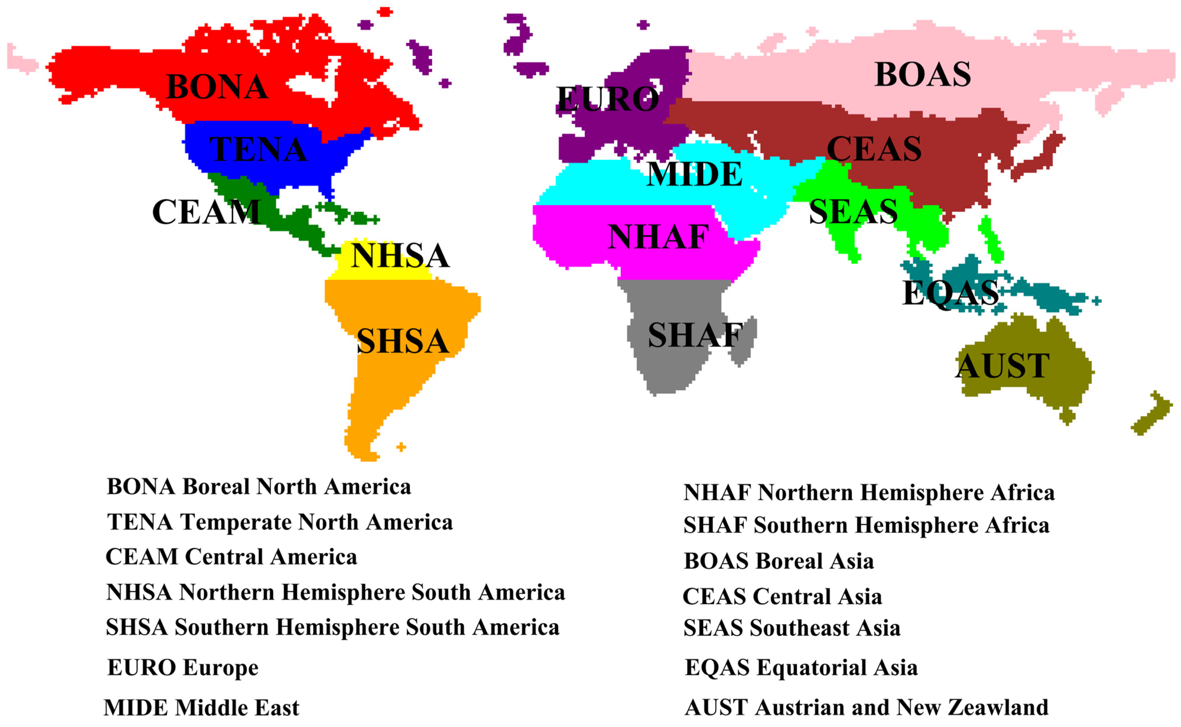
• The SHAF, NHAF, and SHSA regions account for the majority of wildfire occurrences.
• The fusion of global system data and remote correlation indices enhances model capabilities.
• The synergy between spatiotemporal data improves predictive performance.
• Static geographical location information also influences wildfire predictions.
• Treating the prediction task as an image segmentation task is feasible, allowing for attention to be paid to geographical continuity and correlation.

References

1. Bond, W.; Keeley, J. Fire as a Global “Herbivore”: The Ecology and Evolution of Flammable Ecosystems. Trends Ecol. Evol. 2005, 20, 387–394. [Google Scholar] [CrossRef] [PubMed]
2. Bowman, D.M.J.S.; Balch, J.; Artaxo, P.; Bond, W.J.; Cochrane, M.A.; D’Antonio, C.M.; DeFries, R.; Johnston, F.H.; Keeley, J.E.; Krawchuk, M.A.; et al. The Human Dimension of Fire Regimes on Earth. J. Biogeogr. 2011, 38, 2223–2236. [Google Scholar] [CrossRef] [PubMed]
3. Fairman, T.; Bennett, L.; Tupper, S.; Nitschke, C. Frequent Wildfires Erode Tree Persistence and Alter Stand Structure and Initial Composition of a Fire-Tolerant Sub-Alpine Forest. J. Veg. Sci. 2017, 28, 1151–1165. [Google Scholar] [CrossRef]
4. Giglio, L.; Boschetti, L.; Roy, D.; Humber, M.; Justice, C. The Collection 6 MODIS Burned Area Mapping Algorithm and Product. Remote Sens. Environ. 2018, 217, 72–85. [Google Scholar] [CrossRef] [PubMed]
5. Giglio, L.; Randerson, J.T.; van der Werf, G.R. Analysis of Daily, Monthly, and Annual Burned Area Using the Fourth-Generation Global Fire Emissions Database (GFED4). J. Geophys. Res. Biogeosci. 2013, 118, 317–328. [Google Scholar] [CrossRef]
6. Simard, S. Fire Severity, Changing Scales, and How Things Hang Together. Int. J. Wildland Fire 1991, 1, 23. [Google Scholar] [CrossRef]
7. Taylor, S.; Woolford, D.; Dean, C.; Martell, D. Wildfire Prediction to Inform Fire Management: Statistical Science Challenges. Stat. Sci. 2013, 28, 586–615. [Google Scholar] [CrossRef]
8. Forkel, M.; Dorigo, W.; Lasslop, G.; Chuvieco, E.; Hantson, S.; Heil, A.; Teubner, I.; Thonicke, K.; Harrison, S.P. Recent Global and Regional Trends in Burned Area and Their Compensating Environmental Controls. Environ. Res. Commun. 2019, 1, 051005. [Google Scholar] [CrossRef]
9. Aldersley, A.; Murray, S.; Cornell, S. Global and Regional Analysis of Climate and Human Drivers of Wildfire. Sci. Total Environ. 2011, 409, 3472–3481. [Google Scholar] [CrossRef]
10. Coogan, S.C.P.; Robinne, F.-N.; Jain, P.; Flannigan, M.D. Scientists’ Warning on Wildfire—A Canadian Perspective. Can. J. For. Res. 2019, 49, 1015–1023. [Google Scholar] [CrossRef]
11. Lausier, A.M.; Jain, S. Overlooked Trends in Observed Global Annual Precipitation Reveal Underestimated Risks. Sci. Rep. 2018, 8, 16746. [Google Scholar] [CrossRef] [PubMed]
12. Perkins-Kirkpatrick, S.E.; Lewis, S.C. Increasing Trends in Regional Heatwaves. Nat. Commun. 2020, 11, 3357. [Google Scholar] [CrossRef] [PubMed]
13. Ren, L.; Arkin, P.; Smith, T.M.; Shen, S.S.P. Global Precipitation Trends in 1900–2005 from a Reconstruction and Coupled Model Simulations. J. Geophys. Res. Atmos. 2013, 118, 1679–1689. [Google Scholar] [CrossRef]
14. Samuels, R.; Hochman, A.; Baharad, A.; Givati, A.; Levi, Y.; Yosef, Y.; Saaroni, H.; Ziv, B.; Harpaz, T.; Alpert, P. Evaluation and Projection of Extreme Precipitation Indices in the Eastern Mediterranean Based on CMIP5 Multi-Model Ensemble. Int. J. Climatol. 2018, 38, 2280–2297. [Google Scholar] [CrossRef]
15. Moreira, F.; Ascoli, D.; Safford, H.; Adams, M.A.; Moreno, J.M.; Pereira, J.M.C.; Catry, F.X.; Armesto, J.; Bond, W.; Gonzalez, M.E.; et al. Wildfire Management in Mediterranean-Type Regions: Paradigm Change Needed. Environ. Res. Lett. 2020, 15. [Google Scholar] [CrossRef]
16. Thompson, M.P.; Wei, Y.; Calkin, D.E.; O’Connor, C.D.; Dunn, C.J.; Anderson, N.M.; Hogland, J.S. Risk Management and Analytics in Wildfire Response. Curr. For. Rep. 2019, 5, 226–239. [Google Scholar] [CrossRef]
17. Jain, P.; Coogan, S.C.P.; Subramanian, S.G.; Crowley, M.; Taylor, S.; Flannigan, M.D. A Review of Machine Learning Applications in Wildfire Science and Management. Environ. Rev. 2020, 28, 478–505. [Google Scholar] [CrossRef]
18. Fornacca, D.; Ren, G.; Xiao, W. Performance of Three MODIS Fire Products (MCD45A1, MCD64A1, MCD14ML), and ESA Fire_CCI in a Mountainous Area of Northwest Yunnan, China, Characterized by Frequent Small Fires. Remote Sens. 2017, 9, 1131. [Google Scholar] [CrossRef]
19. Kondylatos, S.; Prapas, I.; Ronco, M.; Papoutsis, I.; Camps-Valls, G.; Piles, M.; Fernández-Torres, M.; Carvalhais, N. Wildfire Danger Prediction and Understanding with Deep Learning. Geophys. Res. Lett. 2022, 49, e2022GL099368. [Google Scholar] [CrossRef]
20. Hantson, S.; Arneth, A.; Harrison, S.P.; Kelley, D.I.; Prentice, I.C.; Rabin, S.S.; Archibald, S.; Mouillot, F.; Arnold, S.R.; Artaxo, P.; et al. The Status and Challenge of Global Fire Modelling. Biogeosciences 2016, 13, 3359–3375. [Google Scholar] [CrossRef]
21. Langford, Z.; Kumar, J.; Hoffman, F. Wildfire Mapping in Interior Alaska Using Deep Neural Networks on Imbalanced Datasets; Tong, H., Li, Z., Zhu, F., Yu, J., Eds.; IEEE: New York, NY, USA, 2018; pp. 770–778. [Google Scholar]
22. Shams Eddin, M.H.; Roscher, R.; Gall, J. Location-Aware Adaptive Normalization: A Deep Learning Approach for Wildfire Danger Forecasting. IEEE Trans. Geosci. Remote Sens. 2023, 61, 1–18. [Google Scholar] [CrossRef]
23. Ngoc Thach, N.; Bao-Toan Ngo, D.; Xuan-Canh, P.; Hong-Thi, N.; Hang Thi, B.; Nhat-Duc, H.; Dieu, T.B. Spatial Pattern Assessment of Tropical Forest Fire Danger at Thuan Chau Area (Vietnam) Using GIS-Based Advanced Machine Learning Algorithms: A Comparative Study. Ecol. Inform. 2018, 46, 74–85. [Google Scholar] [CrossRef]
24. Costafreda-Aumedes, S.; Comas, C.; Vega-Garcia, C. Human-Caused Fire Occurrence Modelling in Perspective: A Review. Int. J. Wildland Fire 2017, 26, 983–998. [Google Scholar] [CrossRef]
25. Li, X.; Chen, Z.; Wu, Q.; Liu, C. 3D Parallel Fully Convolutional Networks for Real-Time Video Wildfire Smoke Detection. IEEE Trans. Circuits Syst. Video Technol. 2020, 30, 89–103. [Google Scholar] [CrossRef]
26. Barrett, K.; McGuire, A.D.; Hoy, E.E.; Kasischke, E.S. Potential Shifts in Dominant Forest Cover in Interior Alaska Driven by Variations in Fire Severity. Ecol. Appl. 2011, 21, 2380–2396. [Google Scholar] [CrossRef] [PubMed]
27. Van Le, H.; Hoang, D.A.; Tran, C.T.; Nguyen, P.Q.; Hoang, N.D.; Amiri, M.; Ngo, T.P.; Nhu, H.V.; Van Hoang, T.; Bui, D.T. A New Approach of Deep Neural Computing for Spatial Prediction of Wildfire Danger at Tropical Climate Areas. Ecol. Inform. 2021, 63, 101300. [Google Scholar] [CrossRef]
28. Gholamnia, K.; Nachappa, T.G.; Ghorbanzadeh, O.; Blaschke, T. Comparisons of Diverse Machine Learning Approaches for Wildfire Susceptibility Mapping. Symmetry 2020, 12, 604. [Google Scholar] [CrossRef]
29. Prapas, I.; Ahuja, A.; Kondylatos, S.; Karasante, I.; Panagiotou, E.; Alonso, L.; Davalas, C.; Michail, D.; Carvalhais, N.; Papoutsis, I. Deep Learning for Global Wildfire Forecasting. arXiv 2022, arXiv:2211.00534. [Google Scholar]
30. Shang, C.; Wulder, M.A.; Coops, N.C.; White, J.C.; Hermosilla, T. Spatially-Explicit Prediction of Wildfire Burn Probability Using Remotely-Sensed and Ancillary Data. Can. J. Remote Sens. 2020, 46, 313–329. [Google Scholar] [CrossRef]
31. Denham, M.; Wendt, K.; Bianchini, G.; Cortés, A.; Margalef, T. Dynamic Data-Driven Genetic Algorithm for Forest Fire Spread Prediction. J. Comput. Sci. 2012, 3, 398–404. [Google Scholar] [CrossRef]
32. Hodges, J.; Lattimer, B. Wildland Fire Spread Modeling Using Convolutional Neural Networks. Fire Technol. 2019, 55, 2115–2142. [Google Scholar] [CrossRef]
33. Radke, D.; Hessler, A.; Ellsworth, D. FireCast: Leveraging Deep Learning to Predict Wildfire Spread; International Joint Conferences on Artificial Intelligence Organization: Macao, China, 2019; pp. 4575–4581. [Google Scholar]
34. Huot, F.; Hu, R.L.; Goyal, N.; Sankar, T.; Ihme, M.; Chen, Y.-F. Next Day Wildfire Spread: A Machine Learning Dataset to Predict Wildfire Spreading from Remote-Sensing Data. IEEE Trans. Geosci. Remote Sens. 2022, 60, 1–13. [Google Scholar] [CrossRef]
35. Preisler, H.K.; Westerling, A.L.; Gebert, K.M.; Munoz-Arriola, F.; Holmes, T.P. Spatially Explicit Forecasts of Large Wildland Fire Probability and Suppression Costs for California. Int. J. Wildland Fire 2011, 20, 508–517. [Google Scholar] [CrossRef]
36. Boulanger, Y.; Parisien, M.-A.; Wang, X. Model-Specification Uncertainty in Future Area Burned by Wildfires in Canada. Int. J. Wildland Fire 2018, 27, 164–175. [Google Scholar] [CrossRef]
37. Chen, Y.; Morton, D.C.; Andela, N.; Giglio, L.; Randerson, J.T. How Much Global Burned Area Can Be Forecast on Seasonal Time Scales Using Sea Surface Temperatures? Environ. Res. Lett. 2016, 11, 045001. [Google Scholar] [CrossRef]
38. Lehsten, V.; Harmand, P.; Palumbo, I.; Arneth, A. Modelling Burned Area in Africa. Biogeosciences 2010, 7, 3199–3214. [Google Scholar] [CrossRef]
39. Mayr, M.J.; Vanselow, K.A.; Samimi, C. Fire Regimes at the Arid Fringe: A 16-Year Remote Sensing Perspective (2000–2016) on the Controls of Fire Activity in Namibia from Spatial Predictive Models. Ecol. Indic. 2018, 91, 324–337. [Google Scholar] [CrossRef]
40. Nadeem, K.; Taylor, S.; Woolford, D.; Dean, C. Mesoscale Spatiotemporal Predictive Models of Daily Human- and Lightning-Caused Wildland Fire Occurrence in British Columbia. Int. J. Wildland Fire 2020, 29, 11–27. [Google Scholar] [CrossRef]
41. Amatulli, G.; Rodrigues, M.J.; Trombetti, M.; Lovreglio, R. Assessing Long-Term Fire Risk at Local Scale by Means of Decision Tree Technique. J. Geophys. Res. Biogeosci. 2006, 111, G04S05. [Google Scholar] [CrossRef]
42. Bauer, P.; Thorpe, A.; Brunet, G. The Quiet Revolution of Numerical Weather Prediction. Nature 2015, 525, 47–55. [Google Scholar] [CrossRef]
43. Coffield, S.R.; Graff, C.A.; Chen, Y.; Smyth, P.; Foufoula-Georgiou, E.; Randerson, J.T. Machine Learning to Predict Final Fire Size at the Time of Ignition. Int. J. Wildland Fire 2019, 28, 861–873. [Google Scholar] [CrossRef] [PubMed]
44. Karpatne, A.; Ebert-Uphoff, I.; Ravela, S.; Babaie, H.A.; Kumar, V. Machine Learning for the Geosciences: Challenges and Opportunities. IEEE Trans. Knowl. Data Eng. 2019, 31, 1544–1554. [Google Scholar] [CrossRef]
45. de Bem, P.P.; de Carvalho Junior, O.A.; Trondoli Matricardi, E.A.; Guimaraes, R.F.; Trancoso Gomes, R.A. Predicting Wildfire Vulnerability Using Logistic Regression and Artificial Neural Networks: A Case Study in Brazil’s Federal District. Int. J. Wildland Fire 2019, 28, 35–45. [Google Scholar] [CrossRef]
46. Jaafari, A.; Zenner, E.K.; Panahi, M.; Shahabi, H. Hybrid Artificial Intelligence Models Based on a Neuro-Fuzzy System and Metaheuristic Optimization Algorithms for Spatial Prediction of Wildfire Probability. Agric. For. Meteorol. 2019, 266, 198–207. [Google Scholar] [CrossRef]
47. Oulad Sayad, Y.; Mousannif, H.; Al Moatassime, H. Predictive Modeling of Wildfires: A New Dataset and Machine Learning Approach. Fire Saf. J. 2019, 104, 130–146. [Google Scholar] [CrossRef]
48. Xie, Y.; Peng, M. Forest Fire Forecasting Using Ensemble Learning Approaches. Neural Comput. Appl. 2019, 31, 4541–4550. [Google Scholar] [CrossRef]
49. Iban, M.C.; Sekertekin, A. Machine Learning Based Wildfire Susceptibility Mapping Using Remotely Sensed Fire Data and GIS: A Case Study of Adana and Mersin Provinces, Turkey. Ecol. Inform. 2022, 69, 101647. [Google Scholar] [CrossRef]
50. Pourghasemi, H.R.; Gayen, A.; Lasaponara, R.; Tiefenbacher, J.P. Application of Learning Vector Quantization and Different Machine Learning Techniques to Assessing Forest Fire Influence Factors and Spatial Modelling. Environ. Res. 2020, 184, 109321. [Google Scholar] [CrossRef]
51. Dutta, R.; Aryal, J.; Das, A.; Kirkpatrick, J.B. Deep Cognitive Imaging Systems Enable Estimation of Continental-Scale Fire Incidence from Climate Data. Sci. Rep. 2013, 3, 3188. [Google Scholar] [CrossRef]
52. Shmuel, A.; Heifetz, E. Global Wildfire Susceptibility Mapping Based on Machine Learning Models. Forests 2022, 13, 1050. [Google Scholar] [CrossRef]
53. Yu, Y.; Mao, J.; Thornton, P.E.; Notaro, M.; Wullschleger, S.D.; Shi, X.; Hoffman, F.M.; Wang, Y. Quantifying the Drivers and Predictability of Seasonal Changes in African Fire. Nat. Commun. 2020, 11, 2893. [Google Scholar] [CrossRef] [PubMed]
54. Reichstein, M.; Camps-Valls, G.; Stevens, B.; Jung, M.; Denzler, J.; Carvalhais, N. Prabhat Deep Learning and Process Understanding for Data-Driven Earth System Science. Nature 2019, 566, 195–204. [Google Scholar] [CrossRef] [PubMed]
55. Rusk, N. Deep Learning. Nat. Methods 2016, 13, 35. [Google Scholar] [CrossRef]
56. Nowack, P.; Runge, J.; Eyring, V.; Haigh, J.D. Causal Networks for Climate Model Evaluation and Constrained Projections. Nat. Commun. 2020, 11, 1415. [Google Scholar] [CrossRef] [PubMed]
57. Runge, J.; Bathiany, S.; Bollt, E.; Camps-Valls, G.; Coumou, D.; Deyle, E.; Glymour, C.; Kretschmer, M.; Mahecha, M.; Muñoz-Marí, J.; et al. Inferring Causation from Time Series in Earth System Sciences. Nat. Commun. 2019, 10, 2553. [Google Scholar] [CrossRef] [PubMed]
58. Bergado, J.R.; Persello, C.; Reinke, K.; Stein, A. Predicting Wildfire Burns from Big Geodata Using Deep Learning. Saf. Sci. 2021, 140, 105276. [Google Scholar] [CrossRef]
59. Ham, Y.-G.; Kim, J.-H.; Luo, J.-J. Deep Learning for Multi-Year ENSO Forecasts. Nature 2019, 573, 568. [Google Scholar] [CrossRef]
60. Matsuoka, D.; Nakano, M.; Sugiyama, D.; Uchida, S. Deep Learning Approach for Detecting Tropical Cyclones and Their Precursors in the Simulation by a Cloud-Resolving Global Nonhydrostatic Atmospheric Model. Prog. Earth Planet. Sci. 2018, 5, 1–6. [Google Scholar] [CrossRef]
61. Zhang, G.; Wang, M.; Liu, K. Forest Fire Susceptibility Modeling Using a Convolutional Neural Network for Yunnan Province of China. Int. J. Disaster Risk Sci. 2019, 10, 386–403. [Google Scholar] [CrossRef]
62. Zhu, Q.; Riley, W.J.; Zhao, L.; Xu, L.; Yuan, K.; Chen, M.; Wu, H.; Gui, Z.; Gong, J.; Randerson, J.T. AttentionFire_v1.0: Interpretable Machine Learning Fire Model for Burned-Area Predictions over Tropics. Geosci. Model Dev. 2023, 16, 869–884. [Google Scholar] [CrossRef]
63. Zhang, G.; Wang, M.; Liu, K. Dynamic Prediction of Global Monthly Burned Area with Hybrid Deep Neural Networks. Ecol. Appl. 2022, 32, e2610. [Google Scholar] [CrossRef] [PubMed]
64. Zhang, G.; Wang, M.; Liu, K. Deep Neural Networks for Global Wildfire Susceptibility Modelling. Ecol. Indic. 2021, 127, 107735. [Google Scholar] [CrossRef]
65. Prapas, I.; Bountos, N.I.; Kondylatos, S.; Michail, D.; Camps-Valls, G.; Papoutsis, I. TeleViT: Teleconnection-Driven Transformers Improve Subseasonal to Seasonal Wildfire Forecasting. arXiv 2023, arXiv:2306.10940. [Google Scholar]
66. Bedia, J.; Herrera, S.; Gutierrez, J.M. Assessing the Predictability of Fire Occurrence and Area Burned across Phytoclimatic Regions in Spain. Nat. Hazards Earth Syst. Sci. 2014, 14, 53–66. [Google Scholar] [CrossRef]
67. Joseph, M.; Rossi, M.W.; Mietkiewicz, N.P.; Mahood, A.L.; Cattu, M.E.; St Dents, L.A.; Nagy, R.C.; Iglesias, V.; Abatzoglou, J.T.; Balch, J.K. Spatiotemporal Prediction of Wildfire Size Extremes with Bayesian Finite Sample Maxima. Ecol. Appl. 2019, 29, e01898. [Google Scholar] [CrossRef]
68. Williams, A.P.; Abatzoglou, J.T. Recent Advances and Remaining Uncertainties in Resolving Past and Future Climate Effects on Global Fire Activity. Curr. Clim. Change Rep. 2016, 2, 1–14. [Google Scholar] [CrossRef]
69. Justino, F.; Bromwich, D.H.; Wang, S.-H.; Althoff, D.; Schumacher, V.; Da Silva, A. Influence of Local Scale and Oceanic Teleconnections on Regional Fire Danger and Wildfire Trends. Sci. Total Environ. 2023, 883, 163397. [Google Scholar] [CrossRef]
70. Ronneberger, O.; Fischer, P.; Brox, T. U-Net: Convolutional Networks for Biomedical Image Segmentation; Navab, N., Hornegger, J., Wells, W., Frangi, A., Eds.; Springer: Berlin/Heidelberg, Germany, 2015; Volume 9351, pp. 234–241. [Google Scholar]
71. Li, X.; Wang, W.; Hu, X.; Yang, J. Selective Kernel Networks. arXiv 2019, arXiv:1903.06586. [Google Scholar]
72. Alonso, L.; Gans, F.; Karasante, I.; Ahuja, A.; Prapas, I.; Kondylatos, S.; Papoutsis, I.; Panagiotou, E.; Mihail, D.; Cremer, F.; et al. SeasFire Cube: A Global Dataset for Seasonal Fire Modeling in the Earth System; Zenodo: Geneva, Switzerland, 2022. [Google Scholar]
73. Munoz-Sabater, J.; Dutra, E.; Agusti-Panareda, A.; Albergel, C.; Arduini, G.; Balsamo, G.; Boussetta, S.; Choulga, M.; Harrigan, S.; Hersbach, H.; et al. ERA5-Land: A State-of-the-Art Global Reanalysis Dataset for Land Applications. Earth Syst. Sci. Data 2021, 13, 4349–4383. [Google Scholar] [CrossRef]
74. Artés, T.; Oom, D.; Rigo, D.D.; Durrant, T.H.; Maianti, P.; Libertà, G.; San-Miguel-Ayanz, J. Metadata Record for: A Global Wildfire Dataset for the Analysis of Fire Regimes and Fire Behaviour. Sci. Data 2019, 6, 296. [Google Scholar] [CrossRef]
75. P.W. Team Climate Indices: Monthly Atmospheric and Ocean Time Series: NOAA Physical Sciences Laboratory. Available online: https://psl.noaa.gov/data/climateindices/list/ (accessed on 19 December 2023).
76. Randerson, J.; Van Der Werf, G.; Giglio, L.; Collatz, G.; Kasibhatla, P. Global Fire Emissions Database; Version 4.1 (GFEDv4); Oak Ridge National Laboratory Distributed Active Archive Center: Oak Ridge, TN, USA, 2017. [Google Scholar]
77. Center For International Earth Science Information Network-CIESIN-Columbia University. Gridded Population of the World, Version 4 (GPWv4): Population Density, Revision 11; Socioeconomic Data and Applications Center: Palisades, NY, USA, 2017. [Google Scholar]
78. Veraverbeke, S.; Rogers, B.M.; Goulden, M.L.; Jandt, R.R.; Miller, C.E.; Wiggins, E.B.; Randerson, J.T. Lightning as a Major Driver of Recent Large Fire Years in North American Boreal Forests. Nat. Clim. Chang. 2017, 7, 529–534. [Google Scholar] [CrossRef]
79. Littell, J.S.; McKenzie, D.; Peterson, D.L.; Westerling, A.L. Climate and Wildfire Area Burned in Western U. S. Ecoprovinces, 1916–2003. Ecol. Appl. 2009, 19, 1003–1021. [Google Scholar] [CrossRef] [PubMed]
80. Kale, M.P.P.; Mishra, A.; Pardeshi, S.; Ghosh, S.; Pai, D.S.; Roy, P.S. Forecasting Wildfires in Major Forest Types of India. Front. For. Glob. Chang. 2022, 5, 882685. [Google Scholar] [CrossRef]
81. Taufik, M.; Torfs, P.J.J.F.; Uijlenhoet, R.; Jones, P.D.; Murdiyarso, D.; Van Lanen, H.A.J. Amplification of Wildfire Area Burnt by Hydrological Drought in the Humid Tropics. Nat. Clim. Chang. 2017, 7, 428. [Google Scholar] [CrossRef]
82. Littell, J.S.; Peterson, D.L.; Riley, K.L.; Liu, Y.; Luce, C.H. A Review of the Relationships between Drought and Forest Fire in the United States. Glob. Chang. Biol. 2016, 22, 2353–2369. [Google Scholar] [CrossRef] [PubMed]
83. Hochreiter, S.; Schmidhuber, J. Long Short-Term Memory. Neural Comput. 1997, 9, 1735–1780. [Google Scholar] [CrossRef]
84. Shi, X.; Chen, Z.; Wang, H.; Yeung, D.-Y.; Wong, W.-K.; Woo, W.-C. Convolutional LSTM Network: A Machine Learning Approach for Precipitation Nowcasting. Adv. Neural Inf. Process. Syst. 2015, 28, 802–810. [Google Scholar]
85. Sokolova, M.; Lapalme, G. A Systematic Analysis of Performance Measures for Classification Tasks. Inf. Process. Manag. 2009, 45, 427–437. [Google Scholar] [CrossRef]
86. Tien Bui, D.; Bui, Q.-T.; Nguyen, Q.-P.; Pradhan, B.; Nampak, H.; Trinh, P.T. A Hybrid Artificial Intelligence Approach Using GIS-Based Neural-Fuzzy Inference System and Particle Swarm Optimization for Forest Fire Susceptibility Modeling at a Tropical Area. Agric. For. Meteorol. 2017, 233, 32–44. [Google Scholar] [CrossRef]
87. Freeman, E.A.; Moisen, G.G. A Comparison of the Performance of Threshold Criteria for Binary Classification in Terms of Predicted Prevalence and Kappa. Ecol. Model. 2008, 217, 48–58. [Google Scholar] [CrossRef]
88. Dosovitskiy, A.; Beyer, L.; Kolesnikov, A.; Weissenborn, D.; Zhai, X.; Unterthiner, T.; Dehghani, M.; Minderer, M.; Heigold, G.; Gelly, S.; et al. An Image Is Worth 16 × 16 Words: Transformers for Image Recognition at Scale. arXiv 2021, arXiv:2010.11929. [Google Scholar]
89. Turco, M.; Jerez, S.; Doblas-Reyes, F.J.; AghaKouchak, A.; Carmen Llasat, M.; Provenzale, A. Skilful Forecasting of Global Fire Activity Using Seasonal Climate Predictions. Nat. Commun. 2018, 9, 1–9. [Google Scholar] [CrossRef] [PubMed]
90. Krawchuk, M.A.; Moritz, M.A.; Parisien, M.-A.; Van Dorn, J.; Hayhoe, K. Global Pyrogeography: The Current and Future Distribution of Wildfire. PLoS ONE 2009, 4, e5102. [Google Scholar] [CrossRef] [PubMed]
91. Parks, S.; Holsinger, L.; Panunto, M.; Jolly, W.; Dobrowski, S.; Dillon, G. High-Severity Fire: Evaluating Its Key Drivers and Mapping Its Probability across Western US Forests. Environ. Res. Lett. 2018, 13, 044037. [Google Scholar] [CrossRef]
92. Xiao, C.; Chen, N.; Hu, C.; Wang, K.; Xu, Z.; Cai, Y.; Xu, L.; Chen, Z.; Gong, J. A Spatiotemporal Deep Learning Model for Sea Surface Temperature Field Prediction Using Time-Series Satellite Data. Environ. Model. Softw. 2019, 120, 104502. [Google Scholar] [CrossRef]
93. Bergen, K.J.; Johnson, P.A.; de Hoop, M.V.; Beroza, G.C. Machine Learning for Data-Driven Discovery in Solid Earth Geoscience. Science 2019, 363, 1299. [Google Scholar] [CrossRef]
94. Liang, H.; Zhang, M.; Wang, H. A Neural Network Model for Wildfire Scale Prediction Using Meteorological Factors. IEEE Access 2019, 7, 176746–176755. [Google Scholar] [CrossRef]
Figure 1. According to the division in GFED4, the world is divided into 14 regions.
Forests 15 00216 g001
Figure 2. Global burning area in various regions.
Forests 15 00216 g002
Figure 3. ConvLSTM structure diagram.
Forests 15 00216 g003
Figure 4. Static feature extraction and fusion.
Forests 15 00216 g004
Figure 5. After concatenating static and dynamic variables, the input is fed into the neural network.
Forests 15 00216 g005
Figure 6. The framework of SLA-ConvLSTM.
Forests 15 00216 g006
Figure 7. Receiver operating characteristic (ROC) curves and area under curve (AUC) for five models in 14 regions and globally.
Forests 15 00216 g007
Figure 8. Accuracy box plot based on global grid points.
Forests 15 00216 g008
Figure 9. F1 score box plot based on global grid points.
Forests 15 00216 g009
Figure 10. Precision box plot based on global grid points.
Forests 15 00216 g010
Figure 11. Global fires observed on 10 June 2019.
Forests 15 00216 g011
Figure 12. Global fire predicted by VIT on 10 June 2019.
Forests 15 00216 g012
Figure 13. Global fire predicted by VITi,g on 10 June 2019.
Forests 15 00216 g013
Figure 14. Global fire predicted by ConvLSTM on 10 June 2019.
Forests 15 00216 g014
Figure 15. Global fire predicted by SLA-ConvLSTM on 10 June 2019.
Forests 15 00216 g015
Figure 16. Global fire predicted by SLA-ConvLSTMi,g on 10 June 2019.
Forests 15 00216 g016
Figure 17. On 10 June 2019: the performance comparison of VIT.
Forests 15 00216 g017
Figure 18. On 10 June 2019: the performance comparison of VITi,g.
Forests 15 00216 g018
Figure 19. On 10 June 2019: the performance comparison of ConvLSTM.
Forests 15 00216 g019
Figure 20. On 10 June 2019: the performance comparison of SLA-ConvLSTM.
Forests 15 00216 g020
Figure 21. On 10 June 2019: the performance comparison of SLA-ConvLSTMi,g.
Forests 15 00216 g021
Figure 22. Pixel percentage (%) for each wildfire probability level.
Forests 15 00216 g022
Figure 23. The global distribution of fire danger levels predicted by the VIT model.
Forests 15 00216 g023
Figure 24. The global distribution of fire danger levels predicted by the VITi,g model.
Forests 15 00216 g024
Figure 25. The global distribution of fire danger levels predicted by the ConvLSTM model.
Forests 15 00216 g025
Figure 26. The global distribution of fire danger levels predicted by the SLA-ConvLSTM model.
Forests 15 00216 g026
Figure 27. The global distribution of fire danger levels predicted by the SLA-ConvLSTMi,g model.
Forests 15 00216 g027