Article

Estimation and Spatial Distribution of Individual Tree Aboveground Biomass in a Chinese Fir Plantation in the Dabieshan Mountains of Western Anhui, China

1
School of Environment and Tourism, West Anhui University, Lu’an 237012, China
2
State Key Laboratory of Mountain Hazards and Engineering Safety, Institute of Mountain Hazards and Environment, Chinese Academy of Sciences, Chengdu 610299, China
3
School of Electronic and Information Engineering, West Anhui University, Lu’an 237012, China
*
Authors to whom correspondence should be addressed.
Forests 2024, 15(10), 1743; https://doi.org/10.3390/f15101743
Submission received: 3 September 2024 / Revised: 27 September 2024 / Accepted: 30 September 2024 / Published: 2 October 2024

Abstract

:
Understanding aboveground biomass (AGB) and its spatial distribution is key to evaluating the productivity and carbon sink effect of forest ecosystems. In this study, a 123-year-old Chinese fir forest in the Dabieshan Mountains of western Anhui Province was used as the research subject. Using AGB data calculated from field measurements of individual Chinese fir trees (diameter at breast height [DBH] and height) and spectral vegetation indices derived from unmanned aerial vehicle (UAV) remote sensing images, a random forest regression model was developed to predict individual tree AGB. This model was then used to estimate the AGB of individual Chinese fir trees. Combined with digital elevation model (DEM) data, the effects of topographic factors on the spatial distribution of AGB were analyzed. We found that remote sensing spectral vegetation indices obtained by UAVs can be used to predict the AGB of individual Chinese fir trees, with the normalized difference vegetation index (NDVI) and the optimized soil-adjusted vegetation index (OSAVI) being two important predictors. The estimated AGB of individual Chinese fir trees was 339.34 Mg·ha−1 with a coefficient of variation of 23.21%. At the local scale, under the influence of elevation, slope, and aspect, the AGB of individual Chinese fir trees showed a distribution pattern of decreasing from the middle to the northwest and southeast along the northeast-southwest trend. The effect of elevation on AGB was influenced by slope and aspect; AGB on steep slopes was higher than on gentle slopes, and the impact of slope on AGB was influenced by aspect. Additionally, AGB on north-facing slopes was higher than on south-facing slopes. Our results suggest that local environmental factors such as elevation, slope, and aspect should be considered in future Chinese fir plantation management and carbon sink assessments in the Dabieshan Mountains of western Anhui, China.

1. Introduction

The forest ecosystem is the largest organic carbon pool in terrestrial ecosystems, absorbing and fixing CO2 from the atmosphere through plant photosynthesis [1,2]. As the largest carbon sink on land, forests play a crucial role in balancing regional ecological environments and the global carbon cycle [3,4]. Aboveground forest biomass is a key indicator of forest productivity and carbon sequestration capacity, as well as an important parameter for studying the carbon cycle. Therefore, analyzing the spatial distribution patterns and dynamic changes of forest vegetation carbon storage is of significant importance [5,6]. Forest biomass consists of both aboveground and underground components. Aboveground biomass (AGB), which includes branches, leaves, and trunks, plays a predominant role in evaluating the benefits of the global forest ecosystem. Consequently, estimating forest AGB is essential for understanding the carbon cycle, assessing carbon sink potential, and developing strategies for forest resource management and sustainable forestry development.
The estimation of aboveground biomass (AGB) using traditional field measurements [7,8] and remote sensing [9,10] has been widely employed to evaluate forest productivity and carbon storage [11,12]. Initially, AGB was measured using destructive sampling methods, which involved harvesting, drying, and weighing trees [13]. As research progressed, it was discovered that structural parameters of individual trees, such as diameter at breast height (DBH), basal area, and height, are closely related to AGB, leading to the development and application of allometric growth equations for typical tree species [2]. Although these traditional methods can provide accurate AGB estimates, they are often time-consuming, labor-intensive, costly, and environmentally damaging. They are also not suitable for measuring the spatial distribution of AGB over large areas, especially in remote or rugged mountain environments [14,15].
With the continuous advancement of satellite remote sensing technology, many limitations of traditional estimation methods have been effectively addressed. Using satellite remote sensing to gather forest information minimizes damage to forests and reduces labor and financial costs, allowing for the evaluation of spatial patterns, interannual changes, and long-term trends of forest ecosystems on landscape, regional, and global scales [16,17,18]. Currently, the most widely used remote sensing methods for estimating AGB include (1) optical remote sensing with various spatial resolutions, (2) synthetic aperture radar, and (3) light detection and ranging (LiDAR) technology [19,20,21]. While these technologies have significantly improved overall efficiency, challenges remain due to long revisit periods, cloud contamination, and low spatial resolution [22,23,24].
In recent years, lightweight unmanned aerial vehicle (UAV) remote sensing has addressed some of the limitations of satellite remote sensing technology. UAVs offer advantages such as low cost, high security, high timeliness, high resolution, and low altitude image acquisition, making them increasingly popular for AGB estimation [25,26,27,28]. For instance, Shen et al. [29] utilized multispectral and high-resolution data obtained by UAVs to extract surface information of subtropical natural secondary forests. By combining this with field data, they constructed a stand-scale biomass estimation model to estimate biomass. Similarly, Li and Liu [30] extracted crown information of individual trees from UAV remote sensing images of Pinus sylvestris var. mongolica and, using measured DBH data, developed a crown area-DBH model to estimate AGB on the scale of individual trees. Using airborne LiDAR, Pang and Li [31] estimated the biomass of forest components in the Xiaoxing’an Mountains, finding a significant correlation between LiDAR-extracted variables and biomass of forest components such as stems, branches, and leaves. They suggested that biomass inversion accuracy could be further enhanced by refining regression models through variable selection. Thus, UAV remote sensing technology can provide high-resolution three-dimensional forest structure information at a low cost, making it a promising alternative to aircraft and satellite remote sensing for monitoring forest resources.
When using UAV remote sensing image data to estimate AGB and vegetation coverage, several spectral vegetation indices derived from remote sensing images, such as the normalized difference vegetation index (NDVI), green normalized difference vegetation index (GNDVI), normalized difference red edge (NDRE), leaf chlorophyll index (LCI), and optimized soil-adjusted vegetation index (OSAVI), have been shown to significantly correlate with AGB in numerous studies [14,32,33,34]. Although some studies have successfully estimated the AGB of grasslands and farmlands using a single spectral vegetation index (e.g., NDVI [11,32]) or a combination of a few indices (e.g., NDVI and OSAVI [14,35]), in mountain forests, using only a few spectral indices may limit estimation accuracy due to the influence of environmental conditions (such as soil types, vegetation characteristics, and meteorological conditions) on spectral information [34,36,37,38,39]. Therefore, synthesizing multiple vegetation indices to build an estimation model is necessary to improve model accuracy. The random forest regression model has been demonstrated in many studies to accurately predict biomass using multiple spectral vegetation indices and is suitable for estimating forest AGB [26,40,41,42,43]. In this study, the random forest regression model was employed to estimate the individual tree AGB of Chinese fir.
Forest AGB in mountainous areas exhibits significant spatial variation on a local scale due to factors such as topography, climate, soil, and human activities [44,45,46,47,48], posing challenges for accurately assessing regional forest AGB and its ecological and environmental effects. Thus, many studies emphasize the need to understand the influencing factors when discussing the spatial distribution characteristics of AGB. Topography influences plant growth conditions through various indirect effects [48]. On a landscape and local scale (<1 km2), variations in sunlight, temperature, and precipitation, controlled by elevation, slope, and aspect, affect plant growth [44,49]. For example, in the Northern Hemisphere, slopes facing south receive more solar radiation, resulting in longer growing seasons [50]. Additionally, adiabatic lapse rates due to elevation increase can limit temperature conditions, affecting plant growth [51]. On steep slopes, soil moisture tends to move downslope, causing nutrients such as soil moisture, organic carbon, and nitrogen to accumulate, thereby influencing plant productivity and AGB accumulation [52]. Therefore, more research is needed to verify the influence of topography when studying the spatial distribution of forest AGB in mountainous areas.
Chinese fir (Cunninghamia lanceolata (Lamb.) Hook.), an evergreen conifer in the Cupressaceae family, is a fast-growing native species widely planted in the subtropical hilly areas of China [53]. According to the ninth national forest resources inventory, Chinese fir plantations cover an area of 6.6 million hectares, accounting for 27.23% of the national plantation area, making it the most widely planted species [54]. Chinese fir plantations provide not only substantial commercial timber but also important ecological functions, such as carbon sequestration and water conservation [55]. Dabieshan Mountains in western Anhui is a key ecological barrier in East China. The high-coverage Chinese fir plantation ecosystem effectively protects soil and water resources, regulates the local climate, purifies the environment, and conserves biodiversity. Its carbon sequestration capacity has received increasing attention. To accurately obtain information on individual tree AGB and its spatial distribution in Chinese fir plantations, this study focuses on a 123-year-old Chinese fir plantation with minimal human interference. First, the AGB required for training the random forest regression model was calculated using measured Chinese fir data (DBH and tree height) and an allometric growth model [56] for individual tree AGB. Next, remote sensing spectral vegetation indices (independent variables) and AGB (dependent variables) from measured Chinese fir points obtained by UAVs were used as the training set. A random forest regression was then performed to construct a Chinese fir AGB estimation model based on remote sensing spectral data to estimate individual tree AGB and analyze its spatial distribution characteristics.

2. Materials and Methods
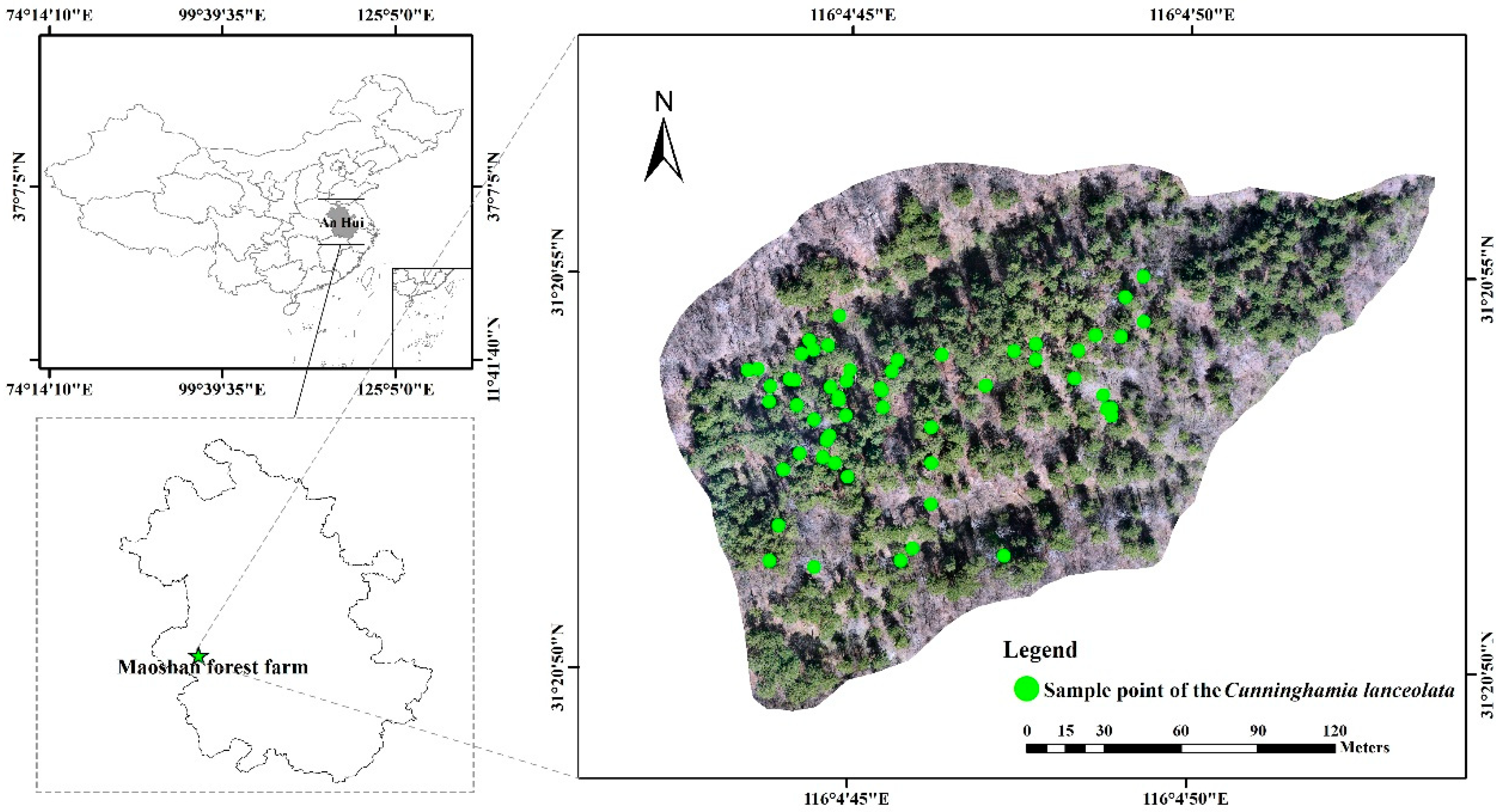
2.1. Study Area

This study was conducted in a Chinese fir plantation at Maoshan Forest Farm (116°4′ E, 31°20′ N) in Huoshan County, western Anhui Province, China (Figure 1). The forest farm covers a total area of 864 hectares, with elevations ranging from 423 to 927 m. The study area is characterized by low mountains and hills, complex topography, variable aspects, slopes of 25–50 degrees, and numerous vertical and horizontal river valleys. This region is located in the northern subtropical warm and humid monsoon climate zone, with an average annual temperature of 15.3 °C and an average annual rainfall of 1366 mm, 44.1% of which occurs in summer. The soils in this area are primarily developed from granite weathering crust and consist mainly of mountain yellow-brown soil and mountain brown soil. The plantations in the forest farm are predominantly pure Chinese fir, mixed forests, and bamboo forests. The study sample plot is a 123-year-old Chinese fir plantation covering 3.86 hectares, planted in 1901 and propagated by cutting.

2.2. Data Collection and Processing

2.2.1. UAV-Based Multispectral Image Data Collection

In this study, a DJI (Shenzhen, China) Mavic 3 UAV equipped with a multispectral camera was used to collect remote sensing image data of the 123-year-old Chinese fir plantation on 29 March 2024. The obtained time of image was the low-value period of low-growth vegetation, which can better distinguish the difference between Chinese fir and others in the study area. The collected images were imported into DJI Terra (Version 4.0.10) for two-dimensional multispectral reconstruction, and visible light image data and five remote sensing vegetation indices (NDVI, GNDVI, NDRE, LCI, and OSAVI) were extracted (Table 1). ENVI 5.3 software was then used to correct the vegetation indices and store these data in a grid format.

2.2.2. Chinese Fir Information Collection

Through filed sampling, we found that the crown width of individual Chinese fir trees ranges around 5 m × 5 m. Based on this, 1644 sampling plots and all raster data were created and processed using ArcGIS 10.8 with a spatial resolution of 5 m × 5 m. Survey points were randomly selected within these plots, with each plot corresponding to one Chinese fir survey point. Fifty-five randomly selected survey points were measured on-site, recording the DBH (cm) of Chinese fir using a DBH ruler and the height (m) using a handheld laser altimeter. The average DBH was 38.83 cm, and the average tree height was 21.26 m.
The vegetation index data (NDVI, GNDVI, NDRE, LCI, and OSAVI) for each sampling plot were extracted using spatial analysis tools in ArcGIS 10.8. The plot value for each sampling point was the average value at the center point, resulting in 1644 data points for each index.

2.3. Calculation of Individual Tree AGB

The allometric growth equation, widely used for biomass estimation, was employed to calculate individual tree AGB. This method establishes the equation by analyzing the relationship between tree characteristics, such as height and DBH, and aboveground biomass, then calculates the AGB based on measured tree characteristic data from field plots [57]. In this study, the allometric growth model for Chinese fir plantations developed by Hou et al. [56] was used to calculate individual tree AGB. The formula used was:
Y = 1.687697 × D 0.571846 × H 1.0803
where Y represents the AGB (Mg·ha−1), D represents the diameter of breast high (cm), and H represents the tree height (m).

2.4. AGB Estimation Model

A model based on UAV-derived spectral vegetation indices was developed to predict the AGB of individual trees in a Chinese fir plantation using random forest regression. Random forest regression is a supervised machine learning algorithm that combines a large number of regression trees, each built from a random subset of one-third of the predictor variables [58]. Because random forest regression is insensitive to collinearity between variables, it ensures prediction accuracy while reducing the risk of overfitting [58]. To optimize model calibration, the number of regression trees is determined by increasing the number until there is no significant improvement in prediction accuracy. The coefficient of determination (R2) and root mean square error (RMSE) are then used to evaluate the model’s accuracy and robustness.
A total of 55 samples were used for model construction, with 80% of the samples serving as the training set to optimize parameters and build the model and 20% as the test set to validate the model. The measured AGB of Chinese fir at 55 survey points was used as the dependent variable (Y), and the corresponding plot values of NDVI, GNDVI, NDRE, LCI, and OSAVI were used as independent variables (X). Random forest regression was performed using the “randomForest” function of the “randomForest” package in R version 4.3.2. First, the importance of each independent variable in the regression process was assessed based on the mean square error increase when the variable was out-of-bag and the impact on model tree node purity when the variable was out-of-bag to select the most relevant independent variables. Second, the number of decision trees in the random forest (ntree) and the number of independent variables randomly selected each time a decision tree was created (mtry) were chosen as parameters to determine the number of regression trees. Various numbers of regression trees were tested, and the relationship between ntree and error was analyzed to determine the optimal value of ntree. Finally, the model’s fit was evaluated using the coefficient of determination (R2) and RMSE. The closer the R2 value is to 1, and the closer the RMSE value is to 0, the higher the model’s prediction accuracy.

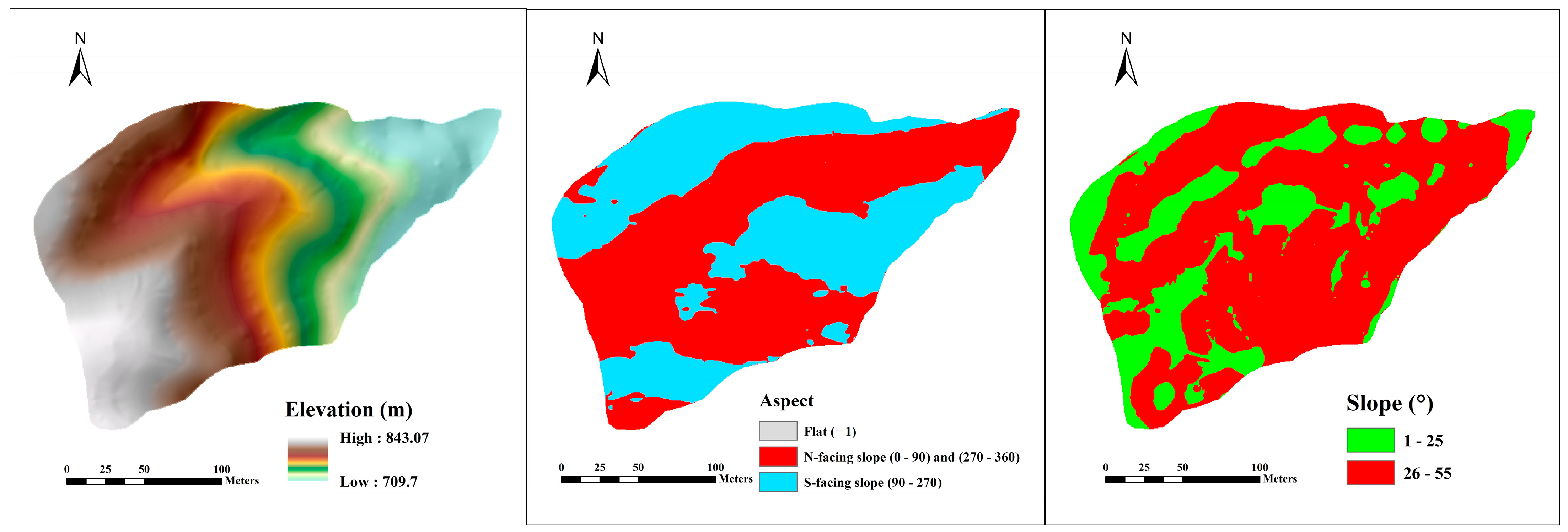
2.5. Acquisition and Classification of Topography Data

Based on a topographic contour map at a scale of 1:500, digital elevation model (DEM) data for the Chinese fir plantation were obtained through geographic registration, digitization, and triangulated irregular network construction, from which slope and aspect information were calculated. Three terrain factors—elevation, slope, and aspect—corresponding to AGB points were extracted using data on the spatial situation of each point. The elevation range of 710–840 m in the study plot was divided into seven gradients (≤720 m, 720–740 m, 740–760 m, 760–780 m, 780–800 m, 800–820 m, and 820–840 m). The slope range of 0–55° was divided into six gradients (0.5°, 6–15°, 16–25°, 26–35°, 36–45°, and 46–55°). Aspect values (−1 to 360) were categorized into nine classes: flat (−1), north ([0, 22.5] and (337.5, 360]), northeast (22.5, 67.5], east (67.5, 112.5], southeast (112.5, 157.5], south (157.5, 202.5], southwest (202.5, 247.5], west (247.5, 292.5], and northwest (292.5, 337.5]. The spatial visualization of topographic factors is shown in Figure 2.

2.6. Statistical Analyses

Before statistical analysis, the Shapiro-Wilk test was used to check if the data were of normal distribution. One-way ANOVA was employed to test whether there were significant differences in AGB among different altitude gradients, slopes, and aspects. LSD tests (p < 0.05) were used for multiple comparisons. Additionally, regression analysis was conducted, using topographic factors (altitude and slope) as independent variables and AGB as the dependent variable, to quantitatively assess the influence of topographic factors on the spatial distribution of biomass. All statistical analyses were performed using R software (version 3.4.3).

3. Results

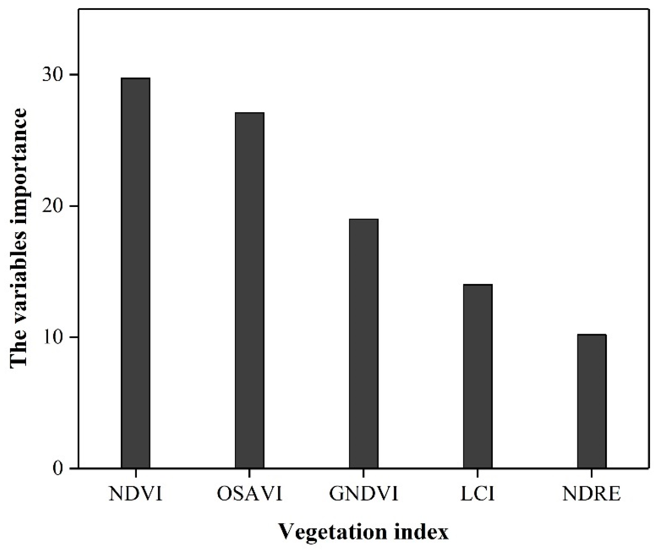
3.1. Random Forest Regression

Based on the calculated aboveground biomass of 55 Chinese fir survey sites (dependent variable Y) and the corresponding vegetation indices of NDVI, GNDVI, NDRE, LCI, and OSAVI (independent variable X), an AGB estimation model based on spectral vegetation indices was established. In this model, the NDVI and OSAVI vegetation indices had the greatest predictive influence, with values of 0.297 and 0.271, respectively (Figure 3). The model demonstrated a good fit, with an R2 of 0.687 and an RMSE of 31.01 Mg·ha−1, indicating its suitability for estimating the AGB of Chinese fir plantations.

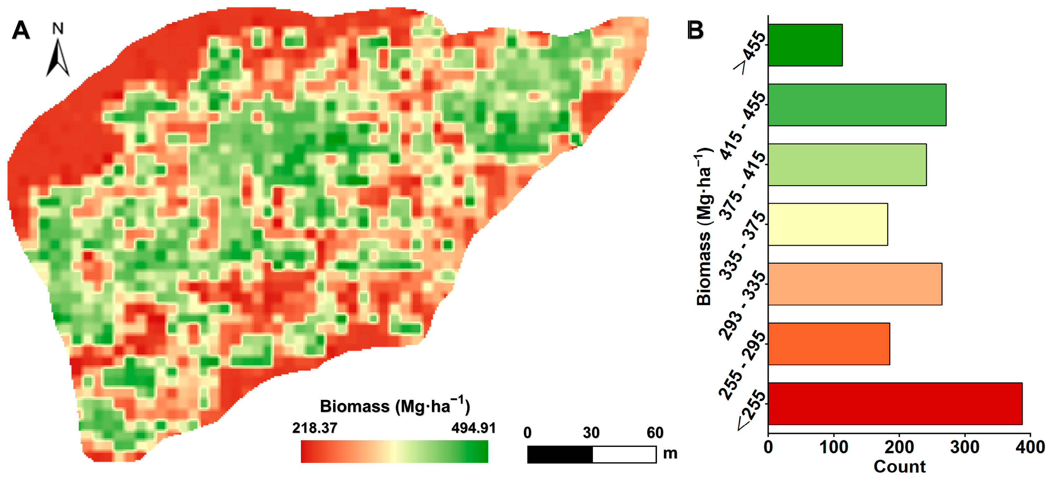
3.2. The AGB of Chinese Fir Plantation

The AGB was calculated using the measured DBH and tree height with the allometric growth model for Chinese fir. Results showed that the average AGB of individual trees in the 123-year-old Chinese fir plantation was 374.89 Mg·ha−1, with a coefficient of variation of 22.87% (Table 2). The estimated individual tree AGB, obtained using the random forest regression model, averaged 339.34 Mg·ha−1, with a coefficient of variation of 23.21% (Table 2). Both measured and estimated AGB values showed significant spatial variation in the individual tree AGB of the Chinese fir plantation, underscoring the need to analyze spatial distribution characteristics and explore influencing factors.

3.3. Spatial Distribution Characteristics of AGB

Spatial visualization of the individual tree AGB of Chinese fir showed a decreasing trend from the center to the northwest and southeast along the northeast-southwest direction (Figure 4). High AGB areas were concentrated in the middle ridge and on the slopes on both sides, while low AGB values were observed in the valley areas at lower altitudes (Figure 2 and Figure 4). The highest AGB areas were mostly located on shady slopes and steep slopes ranging from 25 to 55 degrees (Figure 2 and Figure 4).

3.4. Effect of Topographic Factors on the Spatial Distribution of AGB

One-way ANOVA revealed that elevation significantly influenced the spatial distribution of individual tree AGB in the Chinese fir plantation (p < 0.001). AGB at elevation gradients of 720–740 m, 780–800 m, and 820–840 m was significantly higher than at elevations below 720 m and between 800–820 m (Figure 5), with the highest AGB at the 720–740 m elevation gradient. Similarly, slope also significantly affected the spatial distribution of AGB (p < 0.001), with AGB in slope areas (16–25°) and steep slope areas (26–55°) being significantly higher than in flat slope areas (0–5°) and gentle slope areas (6–15°) (Figure 6). Aspect also significantly impacted the spatial distribution of individual tree AGB (p < 0.001). The highest AGB was found on north-facing slopes, which was significantly greater than on south-facing slopes, southeast-facing slopes, and flat land, with the lowest AGB observed on south-facing slopes. Generally, south-facing and southeast-facing slopes are sunny, while east-facing, southeast-facing, north-facing, and northwest-facing slopes are shady. Therefore, AGB was generally higher on shady slopes than on sunny slopes and flat land (Figure 7).
Further analysis indicated that individual tree AGB in gentle slope areas was highest in the elevation range of 780–800 m, significantly greater than in other elevation ranges, while AGB in the 720–740 m and 800–820 m ranges was the lowest. In contrast, in steep slope areas, AGB was highest in the elevation ranges of 720–740 m and 820–840 m, significantly exceeding other elevation ranges, with the lowest AGB observed in the ≤720 m and 760–780 m ranges. These results suggest that the effect of elevation on biomass is influenced by slope (Figure 8).
The individual tree AGB on flat land was highest in the 780–800 m elevation range, significantly greater than in other elevation ranges, while the 800–820 m range had the lowest AGB. On sunny slopes, AGB in the 740–760 m, 780–800 m, and 820–840 m elevation ranges was significantly higher than in the 760–780 m and 800–820 m ranges. On shady slopes, AGB in the 720–740 m, 780–800 m, and 820–840 m elevation ranges was significantly higher than in other ranges, while AGB in the ≤720 m range was the lowest. These findings indicate that the effect of elevation on AGB is moderated by aspect (Figure 9).
Additionally, there was no significant difference in individual tree AGB across slope intervals on sunny slopes, though a general logarithmic upward trend was observed (y = 17.14 ln(x) + 303.46, R2 = 0.76, p < 0.001). However, on shady slopes, AGB in the 6–15° gentle slope area was significantly lower than in other slope areas, with no obvious overall trend. These results suggest that the effect of slope on AGB is somewhat controlled by aspect (Figure 10).

4. Discussion

4.1. Estimation Effect of Random Forest Regression Model

Many previous studies have demonstrated a significant correlation between spectral vegetation indices derived from remote sensing images and vegetation AGB, which have been successfully used to predict the AGB of crops [14,32,35]. In the 123-year-old Chinese fir plantation in the Dabieshan Mountains of western Anhui, we developed a random forest regression model to predict individual tree AGB using vegetation indices (NDVI, GNDVI, NDRE, LCI, and OSAVI) derived from UAV-obtained remote sensing images. The model showed good performance, with an R2 of 0.687 and an RMSE of 31.01 Mg·ha−1, indicating that vegetation spectral indices can be effectively used to predict individual Chinese fir tree AGB. Our research also found that NDVI and OSAVI had the highest predictive influence among the five vegetation indices tested (Figure 3). Fern et al. highlighted the complementary advantages of NDVI and OSAVI in predicting the AGB of herbs and woody plants in areas with varying vegetation cover or soil reflectivity [35]. Therefore, NDVI and OSAVI should be considered when using vegetation spectral indices to predict the AGB of individual Chinese fir trees.

4.2. Estimated AGB of Individual Chinese Fir Tree

Chinese fir is an important fast-growing timber species in southern China. It is characterized by rapid growth, high yield, and good quality. It is widely distributed and plays a significant role in the subtropical forest ecosystems of China. Therefore, quantifying its productivity and biomass is of great importance [54,55,57]. In this study, the measured average AGB of individual Chinese fir trees in the Dabieshan Mountains area of western Anhui Province was 374.89 Mg·ha−1, while the average AGB estimated using spectral vegetation indices was 339.34 Mg·ha−1. This is close to the result of a previous study, which reported that the individual tree AGB of over-mature Chinese fir forests (≥36 years) was 388.43 Mg·ha−1 [56]. Some studies have noted that when Chinese fir reaches a certain age, its growth rate slows down or even stops. For example, Hou et al. [56] found that the AGB of Chinese fir plantations increased slowly after about 30 years of growth, based on an analysis of AGB data from various regions in China. However, research by Yu et al. [59] on Chinese fir trees of different ages in northern Guangxi showed that growth slows when the trees enter the over-mature stage after 50 years. Additionally, a study conducted at the Mazongling Forest Farm in Jinzhai County, Dabieshan Mountains, western Anhui Province, found that the AGB of 50-year-old Chinese fir trees was lower than that of 45-year-old plantations, with the highest AGB recorded at 392.47 Mg·ha−1 for 48-year-old trees [60]. Therefore, the growth in AGB of the 123-year-old Chinese fir trees in this study may have ceased, considering the potential errors in AGB calculation and local environmental variations in the study area. The results of this study provide a reference for future research on the temporal evolution characteristics of Chinese fir plantation ecosystems.

4.3. Spatial Distribution of Individual Tree AGB

In mountainous environments, topography regulates plant growth conditions such as temperature, light, precipitation, and soil, leading to significant spatial variations in vegetation biomass and distribution characteristics under topographic control [48]. Our study found that the spatial variations in AGB of 123-year-old Chinese fir trees in the Dabieshan Mountains area of western Anhui Province were pronounced. Along the NE-SW trend, AGB showed a decreasing pattern from the center to the northwest and southeast (Table 2 and Figure 4). As predicted, this variation was related to elevation, slope, and aspect.

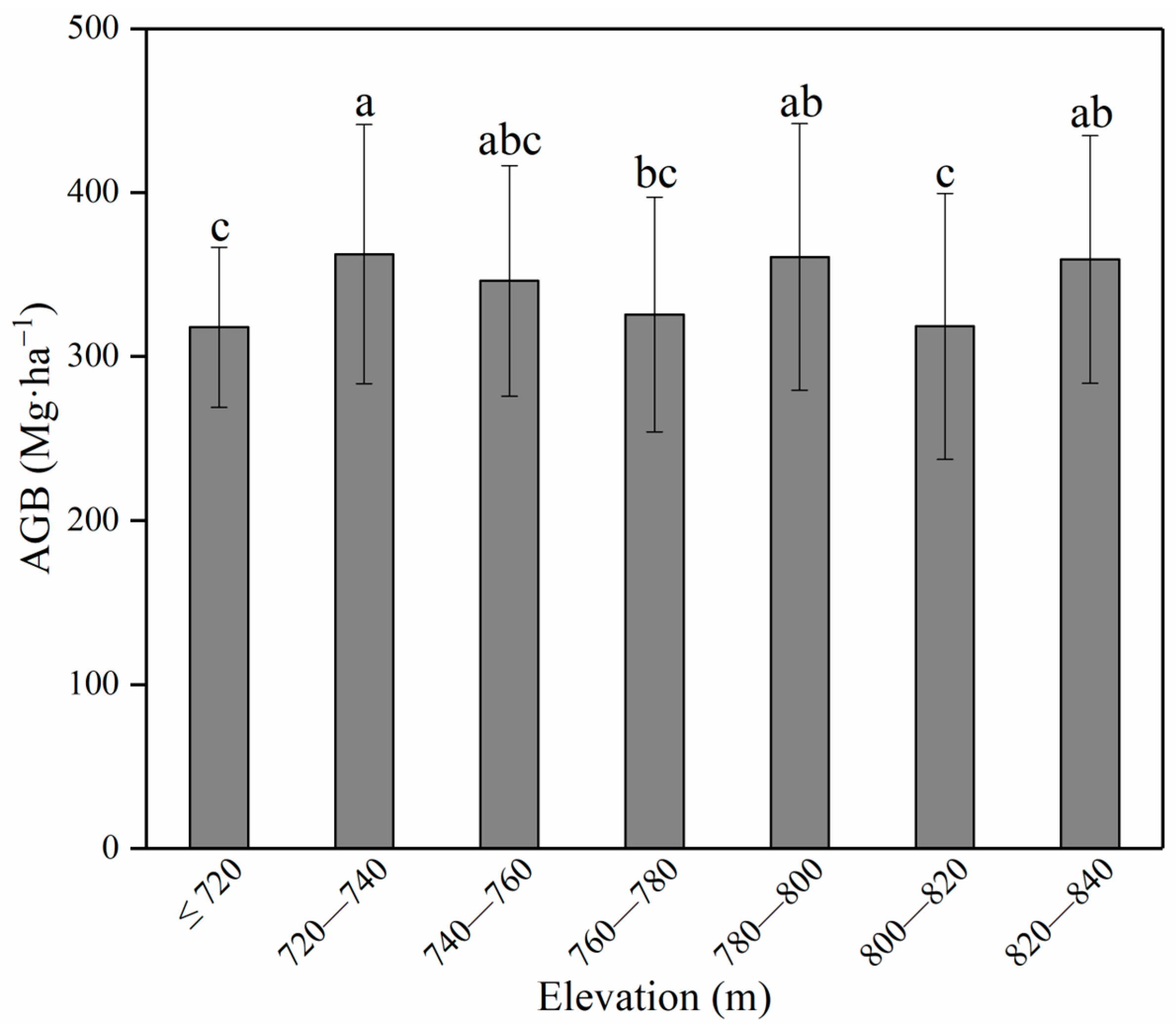
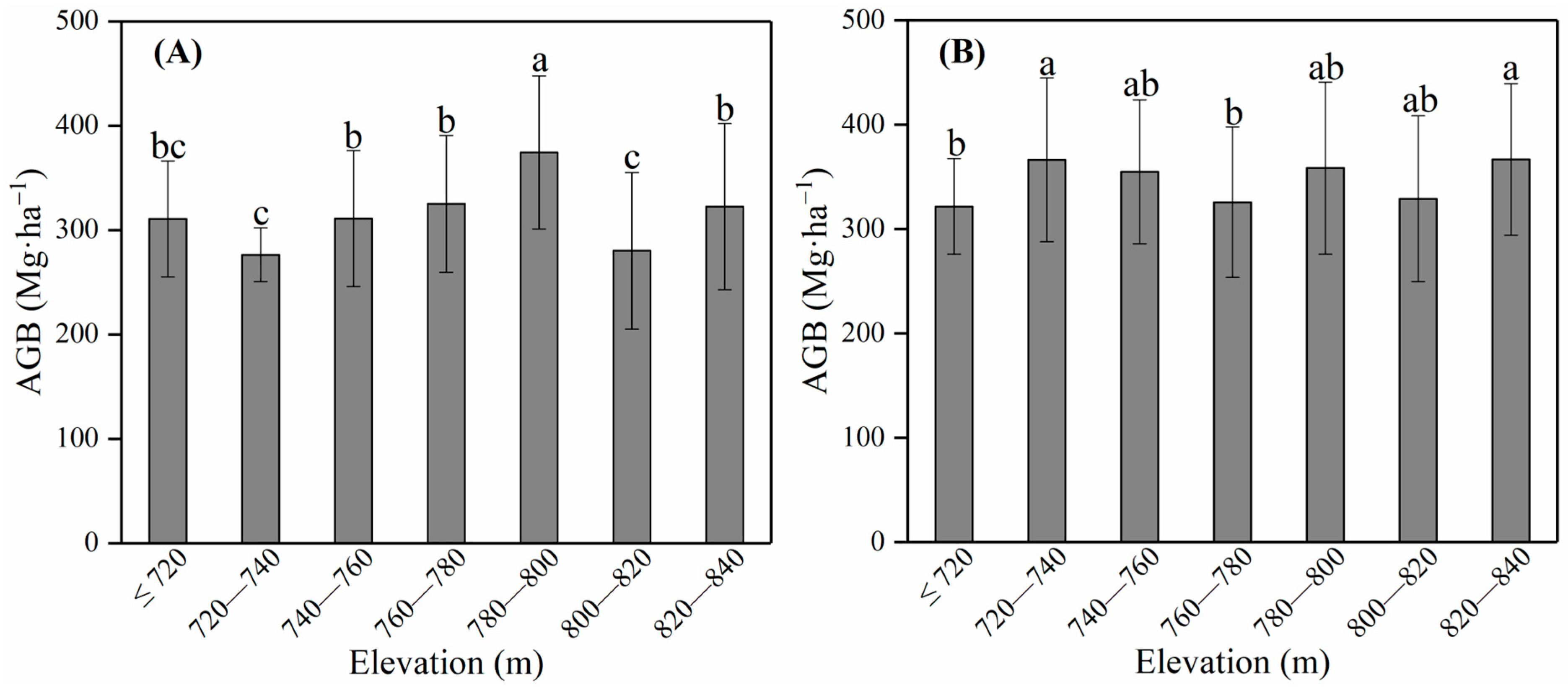
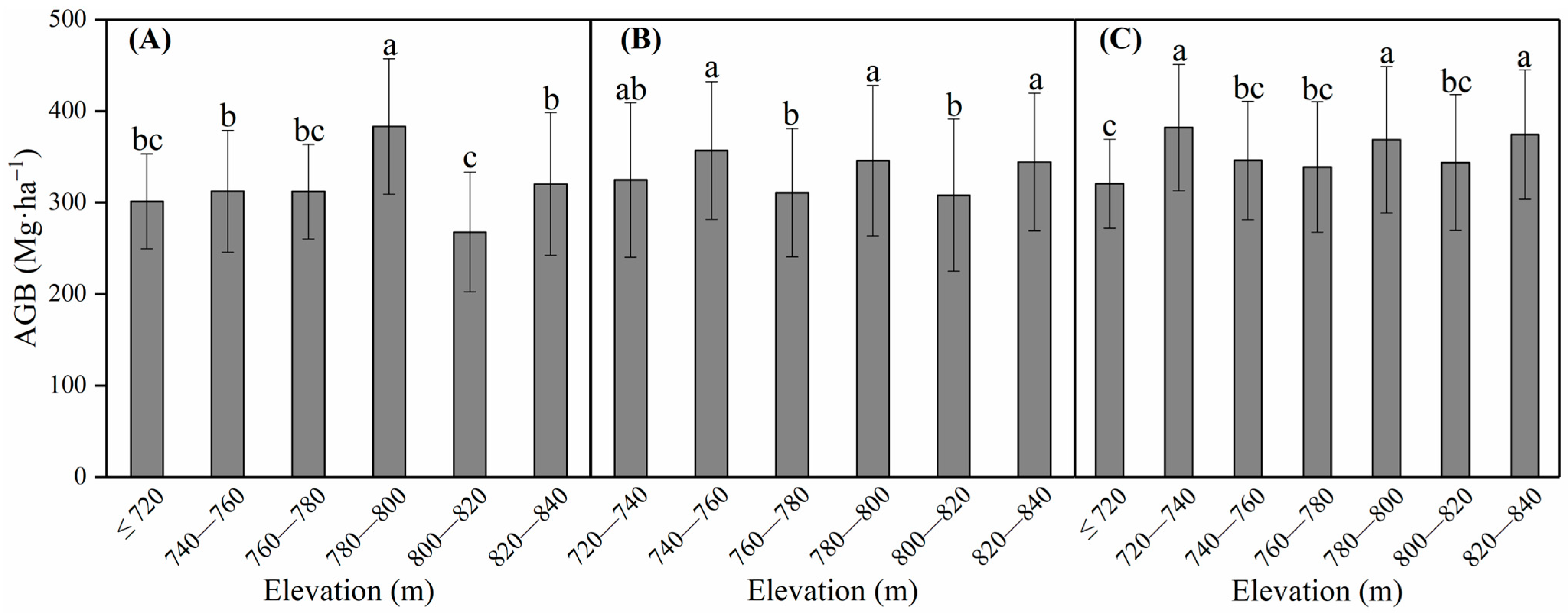
4.3.1. Effect of Elevation

In this study, high AGB values were concentrated at elevation gradients of 720–740 m, 780–800 m, and 820–840 m, while the lowest values were found below 720 m and in gradients of 800–820 m. This differs from the trend observed by Salinas-Melgoza et al., where AGB increased with elevation [61]. This discrepancy may be due to the limited elevation range in our study plot, which makes it difficult to detect a clear trend with elevation. Due to differences in specific ecological environments and research scales, there is still no consensus on the relationship between AGB and elevation gradient [62]. When considering slope, AGB in gentle slope areas was higher at the 780–800 m elevation gradient and lower at 720–740 m and 800–820 m. However, in steep slope areas, AGB was highest at elevation gradients of 720–740 m and 820–840 m and lowest at ≤720 m and 760–780 m (Figure 8). Similar results were confirmed by Yu et al. [63]. This indicates that the influence of elevation on AGB is moderated by slope. Additionally, when considering aspect, there were differences in the elevation gradients where high and low AGB values appeared between shady and sunny slopes, indicating that the influence of elevation on AGB varies with aspect. Therefore, when discussing the spatial distribution characteristics of AGB with respect to elevation, it is necessary to consider the influences of slope and aspect.

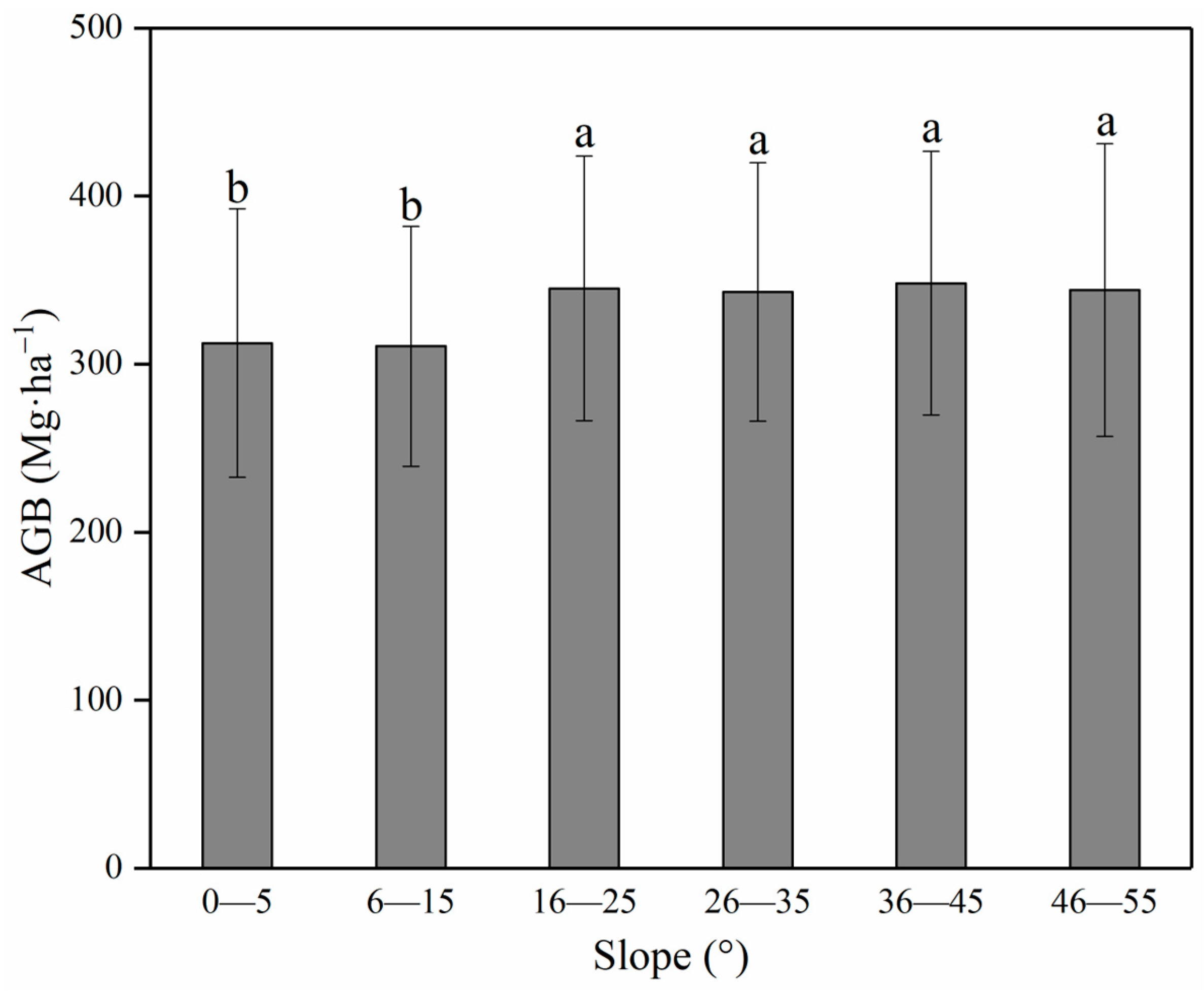
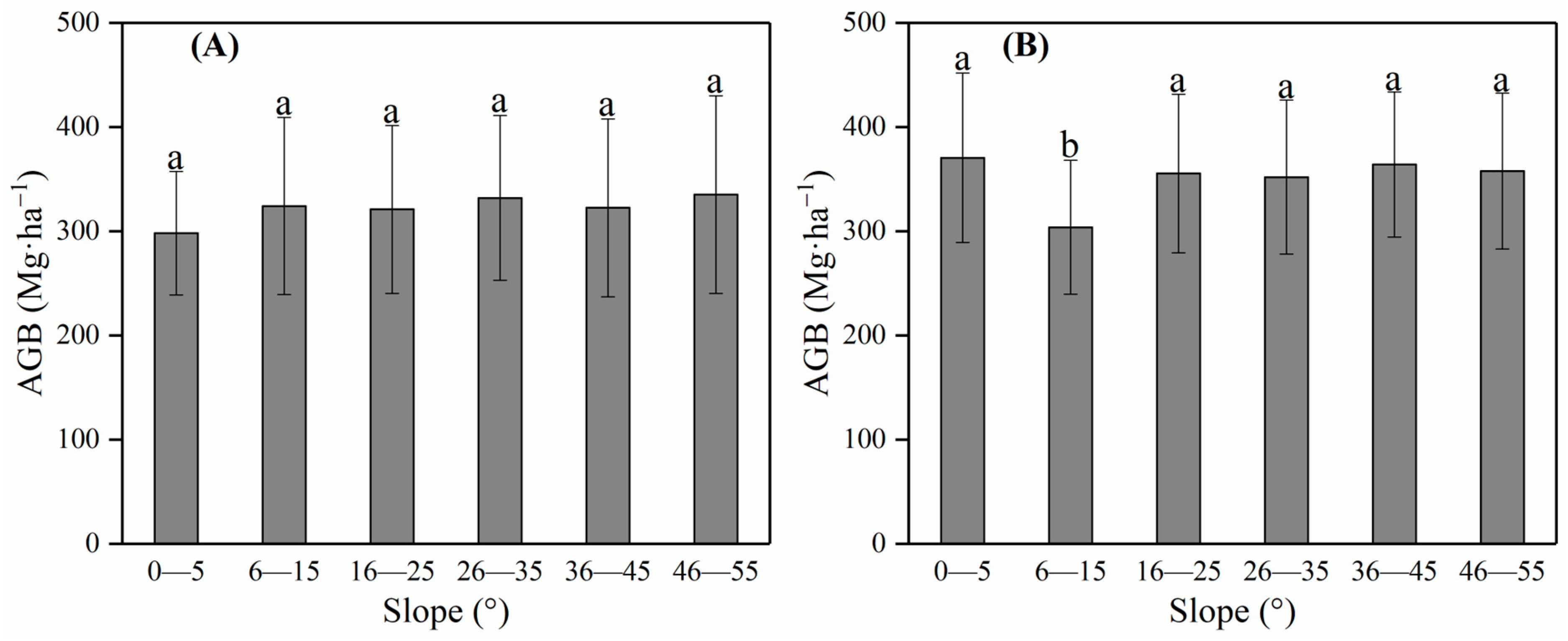
4.3.2. Effect of Slope

Slope has been shown to have an important influence on AGB distribution in many previous studies [64,65,66]. It primarily affects plant growth by causing varying degrees of erosion, impacting soil thickness, soil moisture, and nutrient availability. Additionally, some studies have found that differences in light and heat on different slopes can also affect plant growth in forest environments [64,65]. This study showed that within the 0–55° slope range of Chinese fir plantations, AGB was higher in areas with steeper slopes, consistent with findings from Betula albo-sinensis forests in the Huoditang region of the Qinling Mountains [66]. This may be due to several reasons: (1) steeper slopes increase the area of canopy exposed to light, enhancing CO2 absorption and fixation [65]; (2) the humid climate and improved soil drainage on steeper slopes meet the growth requirements of Chinese fir; and (3) due to long-term protection, the area has good vegetation coverage and a thick litter layer, which prevents destructive soil erosion and nutrient loss even on steep slopes. Additionally, when comparing AGB between different slopes on sunny and shady aspects, we found that AGB on sunny slopes showed a logarithmic increase with slope, while the trend on shady slopes was less pronounced. This suggests that the influence of slope on AGB is moderated by aspect.

4.3.3. Effect of Aspect

Aspect, an important topographic variable, affects the amount and duration of solar radiation received by vegetation, creating local microclimates with different temperatures and water availability, which in turn influences vegetation growth [67]. Generally, slopes facing the poles (shady slopes) are wetter and cooler than those facing the equator (sunny slopes) [68]. In this study, AGB was higher on shady slopes than on sunny slopes, contrary to findings by Ma et al. [66] and Mao et al. [64] in the Qinling and Changbai Mountain forests, respectively. However, some studies in the Northern Hemisphere show that north-facing slopes have higher AGB levels than south-facing slopes [69]. This difference may be related to the growth habits of tree species. According to previous studies, Cunninghamia lanceolata (Lamb.) Hook, in subtropical areas, is a shade-tolerant species that grows better in warm, humid environments with good drainage on shady and semi-shady slopes [70,71]. Therefore, to explain the spatial variation in AGB of Chinese fir trees over the past century, future Chinese fir plantation management in the Dabieshan Mountains area of western Anhui Province should consider the effect of aspect on AGB accumulation.

4.3.4. Suggestion

This study determined that the spatial distribution in the individual tree AGB of the Chinese fir plantation was strongly influenced by the slope and aspect on the local scale. Considering that Chinese fir is widely distributed in hilly areas with complex terrains [53] and is an important commercial timber forest with important ecological functions [55], slope and aspect factors should be considered when planting and managing Chinese fir plantations in mountainous areas with less suitable topographies. In the Dabieshan Mountains area of western Anhui, steep and shady slopes should be given priority as ideal areas for Chinese fir planting to form a natural and suitable forest gap and a shady, humid environment with good drainage, which is beneficial for Chinese fir growth and AGB accumulation. For some gentle slopes or flat lands where Chinese fir does not grow well, the growth environment of Chinese fir can be improved by trimming the slope. Additionally, when we optimize the AGB estimation model in the future, topographic factors (such as elevation, slope and aspect) should be considered as estimation variables.

5. Conclusions

Forest biomass is a key indicator reflecting the productivity, service function, and carbon sink effect of forest ecosystems. Estimating the AGB of individual trees and analyzing their spatial distribution characteristics and influencing factors are essential for understanding the carbon cycle in forest ecosystems and improving forest resource management. In this study, we estimated the AGB of a 123-year-old Chinese fir plantation in the Dabieshan Mountains area of western Anhui Province using AGB data calculated from measured DBH and tree height information, as well as spectral vegetation indices (NDVI, GNDVI, NDRE, LCI, and OSAVI) obtained by UAVs. We discussed the spatial distribution characteristics and topographic influences. We found that remote sensing spectral vegetation indices can be used to predict the AGB of Chinese fir plantations, with NDVI and OSAVI having the highest predictive influence. The predicted average AGB of individual trees in the 123-year-old Chinese fir plantation was 339.34 Mg·ha−1, similar to the AGB of 50-year-old Chinese fir plantations previously measured in this region. On a local scale, the spatial distribution of AGB in the 123-year-old Chinese fir plantation was influenced by elevation, slope, and aspect, showing a pattern of decreasing AGB from the center to the northwest and southeast along the northeast-southwest trend. The influence of elevation on AGB was moderated by slope and aspect. AGB on steep slopes was higher than on gentle slopes, and the influence of slope on AGB was controlled by aspect. Additionally, AGB on shady slopes was higher than on sunny slopes. Therefore, local environmental effects caused by elevation, slope, and aspect should be considered in future Chinese fir plantation management and carbon sink assessments in the Dabieshan Mountains area of western Anhui Province.

Author Contributions

Conceptualization, A.C.; methodology, A.C., X.W. and P.Z.; software, A.C., X.W. and P.Z.; validation, A.C. and X.W.; formal analysis, A.C. and P.Z.; investigation, A.C. and Y.L. (Yongjun Liu); resources, A.C.; data curation, A.C.; writing—original draft preparation, A.C., X.W. and Y.L. (Yongjun Liu); writing—review and editing, Y.L. (Yuanping Li), H.H., G.Z. and T.L.; project administration, A.C.; funding acquisition, A.C. and X.W. All authors have read and agreed to the published version of the manuscript.

Funding

This research was funded by the National Natural Science Foundation of China (grant no. 42301128), the Natural Science Key Research Project of Universities in Anhui Province (grant no. 2022AH051672), the Forestry Carbon Sink Self-Raised Scientific and Technological Research Project of Forestry Bureau in Anhui Province (grant no. 0041122055), the Research Start-Up Fee Project for High-Level Talents in West Anhui University (grant no. WGKQ2021065), and the Natural Science Research Project of West Anhui University (grant no. WXZR202201).

Data Availability Statement

Data will be made available on request.

Acknowledgments

We are very grateful to Liu Jianjun of Maoshan Forest Farm in Huoshan County, for his support and help in our field investigation.

Conflicts of Interest

The authors declare no conflicts of interest.

References

  1. Fang, J.Y.; Guo, Z.D.; Piao, S.L.; Chen, A.P. Terrestrial vegetation carbon sinks in China, 1981−2000. Sci. China Ser. D Earth Sci. 2007, 50, 1341–1350. [Google Scholar] [CrossRef]
  2. Pan, Y.D.; Birdsey, R.A.; Fang, J.Y.; Houghton, R.; Kauppi, P.E.; Kurz, W.A.; Phillips, O.L.; Shvidenko, A.; Lewis, S.L.; Canadell, J.G.; et al. A large and persistent carbon sink in the World’s forests. Science 2011, 333, 988–993. [Google Scholar] [CrossRef] [PubMed]
  3. Piao, S.L.; Yue, C.; Ding, J.Z.; Guo, Z.T. Perspectives on the role of terrestrial ecosystems in the ‘carbon neutrality’ strategy. Sci. China Earth Sci. 2022, 65, 1178–1186. [Google Scholar] [CrossRef]
  4. Yang, Y.H.; Shi, Y.; Sun, W.J.; Chang, J.F.; Zhu, J.X.; Chen, L.Y.; Wang, X.; Guo, Y.P.; Zhang, H.T.; Yu, L.F.; et al. Terrestrial carbon sinks in China and around the world and their contribution to carbon neutrality. Sci. China Life Sci. 2022, 65, 861–895. [Google Scholar] [CrossRef]
  5. Liu, C.F. Remote sensing estimation and spatial and temporal distribution characteristics of forest biomass in the Jianghuai Watershed area. Master’s Thesis, Xinjiang Normal University, Xinjiang, China, 2021. [Google Scholar]
  6. Houghton, R.A. Above ground forest biomass and the global carbon balance. Glob. Chang. Biol. 2005, 11, 945–958. [Google Scholar] [CrossRef]
  7. Fournier, R.A.; Luther, J.E.; Guindon, L.; Lambert, M.C.; Piercey, D.; Hall, R.J.; Wulder, M.A. Mapping aboveground tree biomass at the stand level from inventory information: Test cases in Newfoundland and Quebec. Can. J. For. Res. 2003, 33, 1846–1863. [Google Scholar] [CrossRef]
  8. Parresol, B.R. Assessing tree and stand biomass: A review with examples and critical comparisons. For. Sci. 1999, 45, 573–593. [Google Scholar] [CrossRef]
  9. Zhu, X.L.; Liu, D.S. Improving forest aboveground biomass estimation using seasonal Landsat NDVI time-series. ISPRS J. Photogramm. Remote Sens. 2015, 102, 222–231. [Google Scholar] [CrossRef]
  10. Cutler, M.E.J.; Boyd, D.S.; Foody, G.M.; Vetrivel, A. Estimating tropical forest biomass with a combination of SAR image texture and Landsat TM data: An assessment of predictions between regions. ISPRS J. Photogramm. Remote Sens. 2012, 70, 66–77. [Google Scholar] [CrossRef]
  11. Jiang, F.G.; Kutia, M.; Ma, K.; Chen, S.; Long, J.P.; Sun, H. Estimating the aboveground biomass of coniferous forest in Northeast China using spectral variables, land surface temperature and soil moisture. Sci. Total Environ. 2021, 785, 147335. [Google Scholar] [CrossRef]
  12. Maire, G.L.; Marsden, C.; Nouvellon, Y.; Grinand, C.; Hakamada, R.; Stape, J.; Laclau, J. MODIS NDVI time-series allow the monitoring of Eucalyptus plantation biomass. Remote Sens. Environ. 2011, 115, 2613–2625. [Google Scholar] [CrossRef]
  13. Yang, S.; Feng, Q.; Liang, T.; Liu, B.; Zhang, W.; Xie, H. Modeling Grassland Above-Ground Biomass Based on Artificial Neural Network and Remote Sensing in the Three-River Headwaters Region. Remote Sens. Environ. 2018, 204, 448–455. [Google Scholar] [CrossRef]
  14. Macedo, F.L.; Nóbrega, H.; de Freitas, J.G.R.; Ragonezi, C.; Pinto, L.; Rosa, J.; Pinheiro de Carvalho, M.A.A. Estimation of Productivity and Above-Ground Biomass for Corn (Zea mays) via Vegetation Indices in Madeira Island. Agriculture 2023, 13, 1115. [Google Scholar] [CrossRef]
  15. Soenen, S.A.; Peddle, D.R.; Hall, R.J.; Coburn, C.A.; Hall, F.G. Estimating aboveground forest biomass from canopy reflectance model inversion in mountainous terrain. Remote Sens. Environ. 2010, 114, 1325–1337. [Google Scholar] [CrossRef]
  16. Gleason, C.J.; Im, J. A review of remote sensing of forest biomass and biofuel: Options for small-area applications. GISci. Remote Sens. 2011, 48, 141–170. [Google Scholar] [CrossRef]
  17. Avitabile, V.; Baccini, A.; Friedl, M.A.; Schmullius, C. Capabilities and limitations of Landsat and land cover data for aboveground woody biomass estimation of Uganda. Remote Sens. Environ. 2012, 117, 366–380. [Google Scholar] [CrossRef]
  18. Lu, D.S.; Chen, Q.; Wang, G.X.; Moran, E.; Batistella, M.; Zhang, M.Z.; Vaglio Laurin, G.; Saah, D. Aboveground forest biomass estimation with landsat and LiDAR data and uncertainty analysis of the estimates. Int. J. For. Res. 2012, 2012, 436537. [Google Scholar] [CrossRef]
  19. Wang, G.S.; Wang, N.; Guo, W.L. Modelling Forest Aboveground Biomass Based on GF-3 Dual-Polarized and WorldView-3 Data: A Case Study in Datong National Wetland Park, China. Math. Probl. Eng. 2021, 2021, 9925940. [Google Scholar] [CrossRef]
  20. Li, H.T.; Kato, T.; Hayashi, M.; Wu, L. Estimation of Forest Aboveground Biomass of Two Major Conifers in Ibaraki Prefecture, Japan, from PALSAR-2 and Sentinel-2 Data. Remote Sens. 2022, 14, 468. [Google Scholar] [CrossRef]
  21. Akhtar, A.M.; Qazi, W.A.; Ahmad, S.R.; Gilani, H.; Mahmood, S.A.; Rasool, A. Integration of high-resolution optical and SAR satellite remote sensing datasets for aboveground biomass estimation in subtropical pine forest, Pakistan. Environ. Monit. Asess. 2020, 192, 584. [Google Scholar] [CrossRef]
  22. Jos, G.; Mansor, S.; Matthew, N.K. A Review: Forest Aboveground Biomass (AGB) Estimation Using Satellite Remote Sensing. J. Remote Sens. GIS. 2021, 10, 241. [Google Scholar]
  23. Liang, Y.Y.; Kou, W.L.; Lai, H.Y.; Wang, J.; Wang, Q.H.; Xu, W.H.; Wang, H.; Lu, N. Improved estimation of aboveground biomass in rubber plantations by fusing spectral and textural information from UAV-based RGB imagery. Ecol. Indic. 2022, 142, 109286. [Google Scholar] [CrossRef]
  24. Kou, W.L.; Xiao, X.M.; Dong, J.W.; Gan, S.; Zhai, D.L.; Zhang, G.L.; Qin, Y.W.; Li, L. Mapping Deciduous Rubber Plantation Areas and Stand Ages with PALSAR and Landsat Images. Remote Sens. 2015, 7, 1048–1073. [Google Scholar] [CrossRef]
  25. Mao, P.; Qin, L.J.; Hao, M.Y.; Zhao, W.L.; Luo, J.C.Y.; Qiu, X.; Xu, L.J.; Xiong, Y.J.; Ran, Y.L.; Yan, C.H.; et al. An improved approach to estimate above-ground volume and biomass of desert shrub communities based on UAV RGB images. Ecol. Indic. 2021, 125, 107494. [Google Scholar] [CrossRef]
  26. Tian, Y.C.; Huang, H.; Zhou, G.Q.; Zhang, Q.; Tao, J.; Zhang, Y.L.; Lin, J.L. Aboveground mangrove biomass estimation in Beibu Gulf using machine learning and UAV remote sensing. Sci. Total Environ. 2021, 781, 146816. [Google Scholar] [CrossRef]
  27. Thapa, B.; Lovell, S.; Wilson, J. Remote sensing and machine learning applications for aboveground biomass estimation in agroforestry systems: A review. Agrofor. Syst. 2023, 97, 1097–1111. [Google Scholar] [CrossRef]
  28. Chianucci, F.; Disperati, L.; Guzzi, D.; Bianchini, D.; Nardino, V.; Lastri, C.; Rindinella, A.; Corona, P. Estimation of canopy attributes in beech forests using true colour digital images from a small fixed-wing UAV. Int. J. Appl. Earth Obs. Geoinf. 2016, 47, 60–68. [Google Scholar] [CrossRef]
  29. Shen, X.; Cao, L.; She, G.H. Subtropical forest biomass estimation based on hyperspectral and high-resolution remotely sensed data. J. Remote Sens. 2016, 20, 1446–1460. (In Chinese) [Google Scholar]
  30. Li, B.; Liu, K.N. Forest Biomass Estimation Based on UAV Optical Remote Sensing. For. Eng. 2022, 38, 83–92. (In Chinese) [Google Scholar]
  31. Pang, Y.; Li, Z.Y. Inversion of biomass components of the temperate forest using airborne Lidar technology in Xiaoxing’an Mountains, Northeastern of China. Chin. J. Plant Ecol. 2012, 36, 1095–1105. [Google Scholar] [CrossRef]
  32. Yuan, M.W.; Burjel, J.C.; Martin, N.F.; Isermann, J.; Goeser, N.; Pittelkow, C.M. Advancing on-farm research with UAVs: Cover crop effects on crop growth and yield. Agron. J. 2021, 113, 1071–1083. [Google Scholar] [CrossRef]
  33. Théau, J.; Lauzier-Hudon, É.; Aubé, L.; Devillers, N. Estimation of forage biomass and vegetation cover in grasslands using UAV imagery. PLoS ONE 2021, 16, e0245784. [Google Scholar] [CrossRef]
  34. Li, S.Z.; Xu, D.W.; Fan, K.K.; Chen, J.Q.; Tong, X.Z.; Xin, X.P.; Wang, X. Research of Grassland Aboveground Biomass Inversion based on UAV and Satellite Remoting Sensing. Remote Sen. Technol. Appl. 2022, 37, 272–278. (In Chinese) [Google Scholar]
  35. Fern, R.R.; Foxley, E.A.; Bruno, A.; Morrison, M.L. Suitability of NDVI and OSAVI as estimators of green biomass and coverage in a semi-arid rangeland. Ecol. Indic. 2018, 94, 16–21. [Google Scholar] [CrossRef]
  36. Peng, S.L.; He, N.P.; Yu, G.R.; Wang, Q.F. Aboveground biomass estimation at different scales for subtropical forests in China. Bot. Stud. 2017, 58, 45. [Google Scholar] [CrossRef]
  37. Huete, A.R.; Liu, H.; van Leeuwen, W.J. The use of vegetation indices in forested regions: Issues of linearity and saturation. In Proceedings of the IGARSS’97, 1997 IEEE International Geoscience and Remote Sensing Symposium Proceedings, Remote Sensing—A Scientific Vision for Sustainable Development, Singapore, 3–8 August 1997; pp. 1966–1968. [Google Scholar]
  38. Yang, Q.L.; Su, Y.J.; Hu, T.Y.; Jin, S.C.; Liu, X.Q.; Niu, C.Y.; Liu, Z.H.; Kelly, M.; Wei, J.X.; Guo, Q.H. Allometry-based estimation of forest aboveground biomass combining LiDAR canopy height attributes and optical spectral indexes. For. Ecosyst. 2022, 9, 100059. [Google Scholar] [CrossRef]
  39. Mutanga, O.; Skidmore, A.K. Narrow band vegetation indices overcome the saturation problem in biomass estimation. Int. J. Remote Sens. 2004, 25, 3999–4014. [Google Scholar] [CrossRef]
  40. Zhang, J.; Huang, S.; Hogg, E.H.; Lieffers, V.; Qin, Y.; He, F. Estimating spatial variation in Alberta forest biomass from a combination of forest inventory and remote sensing data. Biogeosciences 2014, 11, 2793–2808. [Google Scholar] [CrossRef]
  41. Mutanga, O.; Adam, E.; Cho, M.A. High density biomass estimation for wetland vegetation using WorldView-2 imagery and random forest regression algorithm. Int. J. Appl. Earth Obs. Geoinf. 2012, 18, 399–406. [Google Scholar] [CrossRef]
  42. Liu, Y.; Lei, P.; You, Q.X.; Tang, X.; Lai, X.; Chen, J.J.; You, H.T. Individual Tree Aboveground Biomass Estimation Based on UAV Stereo Images in a Eucalyptus Plantation. Forests 2023, 14, 1748. [Google Scholar] [CrossRef]
  43. Sun, Z.; Wang, Y.F.; Ding, Z.D.; Liang, R.T.; Xie, Y.H.; Li, R.; Li, H.W.; Pan, L.; Sun, Y.J. Individual tree segmentation and biomass estimation based on UAV Digital aerial photograph. J. Mt. Sci. 2023, 20, 724–737. [Google Scholar] [CrossRef]
  44. Suvanto, S.; Le Roux, P.C.; Luoto, M. Arcticalpine vegetation biomass is driven by fine-scale abiotic heterogeneity. Geogr. Ann. Ser. A Phys. Geogr. 2014, 96, 549–560. [Google Scholar]
  45. Kindermann, G.E.; McCallum, I.; Fritz, S.; Obersteiner, M. A global forest growing stock, biomass and carbon map based on FAO statistics. Silva Fenn. 2008, 42, 387–396. [Google Scholar] [CrossRef]
  46. Tian, X.L.; Xia, J.; Xia, H.B.; Ni, J. Forest biomass and its spatial pattern in Guizhou Province. Chin. J. Appl. Ecol. 2011, 22, 287–294. (In Chinese) [Google Scholar]
  47. Wang, X.L.; Chang, Y.; Chen, H.W.; Hu, Y.M.; Jiao, L.L.; Feng, Y.T.; Wu, W.; Wu, H.F. Spatial pattern of forest biomass and its influencing factors in the Great Xing’an Mountains, Heilongjiang Province, China. Chin. J. Appl. Ecol. 2014, 25, 974–982. (In Chinese) [Google Scholar]
  48. Riihimäki, H.; Heiskanen, J.; Luoto, M. The effect of topography on arctic-alpine aboveground biomass and NDVI patterns. Int. J. Appl. Earth Obs. Geoinf. 2017, 56, 44–53. [Google Scholar] [CrossRef]
  49. Scherrer, D.; Körner, C. Topographically controlled thermal-habitat differentiation buffers alpine plant diversity against climate warming. J. Biogeogr. 2011, 38, 406–416. [Google Scholar] [CrossRef]
  50. Dobrowski, S.Z.; Abatzoglou, J.T.; Greenberg, J.A.; Schladow, S.G. How much influence does landscape-scale physiography have on air temperature in a mountain environment? Agric. For. Meteorol. 2009, 149, 1751–1758. [Google Scholar] [CrossRef]
  51. Dobrowski, S.Z. A climatic basis for microrefugia: The influence of terrain on climate. Glob. Chang. Biol. 2011, 17, 1022–1035. [Google Scholar] [CrossRef]
  52. Stewart, K.J.; Grogan, P.; Coxson, D.S.; Siciliano, S.D. Topography as a key factor driving atmospheric nitrogen exchanges in arctic terrestrial ecosystems. Soil Biol. Biochem. 2014, 70, 96–112. [Google Scholar] [CrossRef]
  53. Zhang, X.Q.; Duan, A.G.; Zhang, J.G. Tree biomass estimation of Chinese fir (Cunninghamia lanceolata) based on Bayesian method. PLoS ONE 2013, 8, e79868. [Google Scholar] [CrossRef] [PubMed]
  54. Qu, Y.C.; Jiang, Y.H.; Chen, H.Y.; Zhang, J.G.; Zhang, X.Q. Dynamic change of stand leaf area for Chinese fir plantation. Acta Ecol. Sin. 2024, 44, 5609–5620. (In Chinese) [Google Scholar]
  55. Zeng, Y.L.; Wu, H.L.; Ouyang, S.; Chen, L.; Fang, X.; Peng, C.H.; Liu, S.R.; Xiao, W.F.; Xiang, W.H. Ecosystem service multifunctionality of Chinese fir plantations differing in stand age and implications for sustainable management. Sci. Total Environ. 2021, 788, 147791. [Google Scholar] [CrossRef] [PubMed]
  56. Hou, Z.H.; Zhang, X.Q.; Xu, D.Y.; Yu, P.T. Study on biomass and productivity of Chinese fir plantation. Chin. Agric. Sci. Bull. 2009, 25, 97–103. [Google Scholar]
  57. Muukkonen, P. Generalized allometric volume and biomass equations for some tree species in Europe. Eur. J. For. Res. 2007, 126, 157–166. [Google Scholar] [CrossRef]
  58. Breiman, L. Random Forest. Mach. Learn. 2001, 45, 5–32. [Google Scholar] [CrossRef]
  59. Yu, Y.F.; Song, T.Q.; Zeng, F.P.; Peng, W.X.; Wen, Y.G.; Huang, C.B.; Wu, Q.B.; Zeng, Z.X.; Yu, Y. Dynamic changes of biomass and its allocation in Cunninghamia lanceolata plantations of different stand ages. Chin. J. Ecol. 2013, 32, 1660–1666. (In Chinese) [Google Scholar]
  60. Shi, W.T.; Xie, X.Y.; Liu, X.J.; Zhang, C.; Ke, L.; Xu, X.N. Biomass model and carbon storage of Chinese fir plantation in Dabieshan Mountains in Anhui. Resour. Environ. Yangtze Basin 2015, 24, 758–764. (In Chinese) [Google Scholar]
  61. Salinas-Melgoza, M.A.; Skutsch, M.; Lovett, J.C. Predicting aboveground forest biomass with topographic variables in human-impacted tropical dry forest landscapes. Ecosphere 2018, 9, e02063. [Google Scholar] [CrossRef]
  62. Zhang, M.; Wang, X.L.; Ma, Y.S.; Wang, Y.L.; Qin, J.P.; Dong, R.Z. Characteristics of the aboveground biomass and diversity along altitudinal gradients in alpine meadows of the upper reaches of the Yarlung Zangbo River. Acta Bot. Boreal. Occident. Sin. 2024, 44, 0154–0163. [Google Scholar]
  63. Yu, S.J.; Wang, J.; He, H.Y.; Zhang, C.Y.; Zhao, X.H. Driving factors of the temporal stability of biomass of broadleaf-conifer forest. Sci. Silvae Sin. 2022, 58, 181–190. (In Chinese) [Google Scholar]
  64. Mao, X.G.; Fan, W.Y.; Li, M.Z.; Yu, Y.; Yang, J.M. Temporal and spatial analysis of forest biomass in Changbai Mountains, Heilongjiang, China. Chin. J. Plant Ecol. 2011, 35, 371–379. (In Chinese) [Google Scholar] [CrossRef]
  65. Shen, B.; Dang, K.L.; Wu, P.H.; Zhu, C.G. Organic carbon density in Pinus tabulaeformis forest ecosystem on the south slope of the middle Qinling Mountains, China. Acta Ecol. Sin. 2015, 35, 1798–1806. (In Chinese) [Google Scholar]
  66. Ma, J.; Dang, K.L.; Wang, L.H.; Yang, S.T. Research on the changes in biomass and volume of Betula albo-sinensis forest at Huoditang region. J. Northwest For. Univ. 2016, 31, 204–210. (In Chinese) [Google Scholar]
  67. Bennie, J.; Huntley, B.; Wiltshire, A.; Hill, M.O.; Baxter, R. Slope, aspect and climate: Spatially explicit and implicit models of topographic microclimate in chalk grassland. Ecol. Model. 2008, 216, 47–59. [Google Scholar] [CrossRef]
  68. Kumari, N.; Saco, P.M.; Rodriguez, J.F.; Johnstone, S.A.; Srivastava, A.; Chun, K.P.; Yetemen, O. The grass is not always greener on the other side: Seasonal reversal of vegetation greenness in aspect-driven semiarid ecosystems. Geophys. Res. Lett. 2020, 47, e2020GL088918. [Google Scholar] [CrossRef]
  69. Kariuki, M.; Rolfe, M.; Smith, R.G.B.; Vanclay, J.K.; Kooyman, R.M. Diameter growth performance varies with species functional-group and habitat characteristics in subtropical rainforests. For. Ecol. Manag. 2006, 225, 1–14. [Google Scholar] [CrossRef]
  70. Chi, J. The comparison of ecological habit between Pinus massoniana and Cunninghamia lanceolata. Hunan For. Sci. Technol. 1992, 19, 31–35. (In Chinese) [Google Scholar]
  71. Yu, X.T. Agroforestry of Chinese fir. Chin. J. Ecol. 1991, 10, 25–28. (In Chinese) [Google Scholar]
Figure 1. The locations of the study area and sampling sites.
Forests 15 01743 g001
Figure 2. Topographic factors of study area.
Forests 15 01743 g002
Figure 3. Importance of vegetation index.
Forests 15 01743 g003
Figure 4. Spatial distribution of individual tree AGB (A) map of individual tree AGB and (B) the number of plots in different biomass groups.
Forests 15 01743 g004
Figure 5. The individual tree AGB on different elevations. The groups with the same letters indicate no significant differences between different elevation gradients (LSD test, p < 0.05). Error bars denote the standard deviation of the mean.
Forests 15 01743 g005
Figure 6. The individual tree AGB on different slopes. The groups with the same letters indicate no significant differences between different slopes (LSD test, p < 0.05). Error bars denote the standard deviation of the mean.
Forests 15 01743 g006
Figure 7. The individual tree AGB on different aspects. The groups with the same letters indicate no significant differences between different aspects (LSD test, p < 0.05). Error bars denote the standard deviation of the mean.
Forests 15 01743 g007
Figure 8. Effect of elevation with different slopes on AGB (A) gentle slope (≤16°); (B) steep slope (>16°). The groups with the same letters indicate no significant differences between different elevation gradients (LSD test, p < 0.05). Error bars denote the standard deviation of the mean.
Forests 15 01743 g008
Figure 9. The effect of elevation with different aspects on AGB (A) flat (B) sunny slope (C) shady slope. The groups with the same letters indicate no significant differences between different elevation gradients (LSD test, p < 0.05). Error bars denote the standard deviation of the mean.
Forests 15 01743 g009
Figure 10. The effect of slope with different aspects on AGB (A) sunny slope; (B) shady slope. The groups with the same letters indicate no significant differences between different slopes (LSD test, p < 0.05). Error bars denote the standard deviation of the mean.
Forests 15 01743 g010
Table 1. Vegetation indices and their calculation formulas [34].
Vegetation IndexFull NameFormula
NDVINormalized Difference Vegetation
Index
(Nir − Red)/(Nir + Red)
GNDVIGreen Normalized Difference Vegetation Index(Nir − Green)/(Nir + Green)
NDRENormalized Difference Red Edge(Nir − RedEdge)/(Nir + RedEdge)
LCILeaf Chlorophyll Index(Nir − RedEdge)/(Nir + Red)
OSAVIOptimized Soil Adjusted Vegetation Index(Nir − Red)/(Nir + Red + 0.16)
Note: Nir indicates near-infrared reflectance, Red indicates red reflectance, Green indicates green reflectance and RedEdge indicates red edge reflectance.
Table 2. Measured and estimated AGB of individual Chinese fir tree (Mg·ha−1).
Individual Tree AGBSample SizeMinimum ValueMaximum ValueMean
Value
Standard DeviationCoefficient of Variation
Measured55180.36614.14374.8985.7222.87%
Estimated1644218.37494.91339.3478.7523.21%
Disclaimer/Publisher’s Note: The statements, opinions and data contained in all publications are solely those of the individual author(s) and contributor(s) and not of MDPI and/or the editor(s). MDPI and/or the editor(s) disclaim responsibility for any injury to people or property resulting from any ideas, methods, instructions or products referred to in the content.

