Windbreak Effectiveness of Single and Double-Arranged Shelterbelts: A Parametric Study Using Large Eddy Simulation

Abstract

Shelterbelts provide essential protection against wind erosion and soil degradation, as well as protection for fruit-bearing plants and crops from strong winds. Enhancing their sheltering capabilities requires optimizing their pattern and orientation, as well as defining their height and desired canopy shape, according to the desired performance. In this work, Large Eddy Simulation is employed to investigate the flow field and windbreak effectiveness of single and double-arranged shelterbelts characterized by different geometry and resistance to the air passage for neutral atmospheric condition. In particular, the canopy of the shelterbelts is modeled as an isotropic porous medium immersed in atmospheric boundary layer flow using the Darcy–Forchheimer model. Results show that a shelterbelt with a rectangular-shaped cross-section and a large canopy height results in the most significant reduction in mean wind speed and TKE, thus providing a large wind-protection region. As the spacing distance of double-arranged shelterbelts increases, the protection zones formed by both shelterbelts are reduced. The systematic comparisons of flow patterns, drag force coefficients, and windbreak effectiveness indicators of a series of single and double-arranged shelterbelts are essential for optimizing the design and management of shelterbelts.

1. Introduction

Shelterbelts, commonly referred to as windbreaks, are critical components of agroecosystems and natural landscapes, providing essential protection against wind erosion [1,2], soil degradation [3,4], and other eco-environmental challenges [5,6]. The efficiency of shelterbelts in altering wind flow patterns and mitigating wind speed is influenced by a range of parameters, which can be categorized into internal and external structural characteristics [7,8]. The geometry, density, and arrangement of individual vegetative elements play a pivotal role in defining the internal structural characteristics of a shelterbelt. External structural characteristics of a shelterbelt, such as width, length, height, cross-sectional shape, and orientation, further define its overall design [7]. The effects of the shelterbelt width, length, opening length, and arrangement pattern were studied by Wang et al. (2024) [9]. However, a detailed and comprehensive understanding of the effects of the canopy shape, canopy height, and spacing distance for multi-shelterbelt systems and, in particular, their impact on shelterbelt efficiency is still missing, with findings in the literature often showing inconsistencies.

In particular, for the case of an isolated shelterbelt, Wang and Takle (1997) [10] revealed that various shelterbelt shapes (i.e., rectangular, triangular, and streamlined profiles) exhibited nearly identical reductions in wind speed and turbulence intensity. Consistent results were also observed in wind tunnel studies conducted by Woodruff and Zingg (1953) [11]. However, Guan et al. (1995) [12] reported that the protective range of a shelterbelt with a rectangular cross-section exceeded that of a trapezoidal shape in wind tunnel experiments. Field observations of model windbreaks further suggested that shelterbelts with a rectangular cross-sectional shape exhibit superior shelter effectiveness [8].

When multiple shelterbelts are considered, as is usually the case in applications, other parameters come into play. In particular, the spacing is the most important design parameter for multiple shelterbelts [13,14,15]. In particular, Woodruff (1956) [16] observed that the wind reduction area between a seven-row principal belt and one- to three-row supplemental belts initially increases and then decreases as the spacing distance between them increases in the range between 11.7 and 24.3 times the height of tallest tree in the belt. Similar results are reported by Frunk and Ruck (2005) [17] in their investigation of the wind reduction provided by double-arranged shelterbelts mounted on mounds. However, Sun et al. (2022) [15] indicated that the protective effect decreases as the spacing interval between principal shelterbelts increase from 10 to 30 times the height of the shelterbelt. A summary of the studies which address the characterization of the aerodynamic efficiency for single shelterbelts is provided in

Table 1. Previous studies on single shelterbelts with different canopy shapes.

	Method	Exposure	Scale	Shelterbelt Height H	Shelterbelt Width W	Shelterbelt Length L	Canopy Shape	Porosity
Woodruff and Zingg (1953) [11]	Wind tunnel test	Gravel floor	1:60	10–30 feet	5, 7, 10 rows	/	Triangular-like	/
Wang and Takle (1997) [10]	Numerical simulation	Atmospheric boundary layer flow	/	10 m	10 m	≫10 m	Rectangular, triangular, streamlined	50%
Guan et al. (1995) [12]	Wind tunnel test	/	/	2–10 cm	15 cm	/	Rectangular, trapezoid	66%
Zhu (2008) [8]	Field test	/	1:1	1.85 m	7 rows	/	Rectangular, triangular, gable roof, notch	60%

, while those concentrating on multiple shelterbelts are summarized in

Table 2. Previous studies on multiple shelterbelts with different spacing distances.

	Method	Exposure	Scale	Shelterbelt Height H	Shelterbelt Width W	Shelterbelt Length L	Spacing Distance s	Porosity
Woodruff (1956) [16]	Wind tunnel test	Sieved gravel floor	1:60	10–30 feet	1–7 row	/	330–729 feet	/
Frunk and Ruck (2005) [17]	Wind tunnel test	Suburban terrain and forested areas, α = 0.26	1:200	12 m	1.2 m	300 m	120 m, 144 m, 240 m, 288 m, 360 m, 480 m, 600 m	0, 12%, 22%, 35%, 52%
Sun et al. (2022) [15]	Field test	Open terrain	1:1	10 m	/	/	100 m, 150 m, 200 m, 250 m, 300 m	40%

.

Coming now to the methodologies which can be used to support the aerodynamic characterization of shelterbelts, we mention field measurements [18,19], wind tunnel tests, [20,21] and Computational Fluid Dynamics (CFD) simulations [22,23,24,25]. In particular, field measurements are extremely useful, but a dedicated measurement campaign is very expensive and hard to carry out in an uncontrolled flow condition. Additionally, they cannot be used to explore different solutions during the design phase. Wind tunnel experiments represent the current state of the art, but generally only allow for measuring velocity in a few locations and struggle in representing porous elements, as the trees’ canopy. The use of CFD simulations can potentially solve many of such shortcomings, as they allow for the monitoring of velocity at every point within the computational domain with ease, and parametrically vary the shelterbelt parameters in a well-controllable way. However, the modeling of shelterbelts is not without challenges in CFDs simulations. In particular, the flow needs to be greatly simplified, usually idealizing the canopy as a porous material. Despite such difficulties, CFD simulations have emerged as a popular tool to study the windbreak effects of shelterbelts [9,24,25,26]. Reynolds-averaged Navier–Stokes (RANS) and Large Eddy Simulation (LES) are two commonly used turbulence models. The former excels in computational efficiency for simulating steady flows, while the latter is better suited for capturing turbulent structures and small-scale turbulence. Many researchers have applied RANS turbulence models to simulate the airflow around shelterbelts [27,28]. Other studies [24,25,29,30] employed LES to evaluate turbulent flow near shelterbelt canopies which, as expected, has shown superior accuracy in simulating the flow patterns in the leeward region of canopies compared to RANS models [24].

In the present paper, a comprehensive numerical study regarding the impact of the parameters which affect the shelterbelts efficiency is performed using LES. In particular, the present paper aims at significantly extending the numerical results already presented in Wang et al. (2024) [9], which concentrated on the shelterbelt height and pattern, by considering the shelterbelt canopy shape and height from the ground, as well as the distance between shelterbelts. Systematic parametric studies are thus performed, independently varying the aforementioned parameters, in order to quantify their effect on the drag forces and the shelterbelts protective effectiveness. It is found that the actual shelterbelt canopy shape plays a limited role with respect to its performance, the most important parameter being the canopy volume. Finally, some simplified formulas are provided, aiming at interpolating the obtained results, which might be useful for obtaining an expedited prediction of the shelterbelts performance.

2. LES Method

2.1. Numerical Models

For numerical validation in this study, the wind field measurements around a shelterbelt (Tsuijimatsu) in Izumo, Japan [18] were utilized. The details of the shelterbelt dimensions and wind speed measurements can be found in Kurotani et al. (2001) [18] and Wang et al. (2024) [9]. Based on the shelterbelt model in Kurotani et al. (2001) [18], three sets of analyses, designated as Cases I to III, were conducted to investigate the effects of the most important parameters on the windbreak effectiveness of single and double-arranged shelterbelts.

In particular, Case I aims to investigate the effect of the cross-sectional shape of the canopy. For this purpose, in addition to the rectangular cross-section similar to that used in Kurotani et al. (2001) [18] (denoted as R-shapes), four other shapes were considered, i.e., windward triangle (WT), leeward triangle (LT), symmetrical triangle (ST1), and streamlined triangle (ST2). The base width of all canopies was kept at W = 2 m, and the canopy height was kept at H_c = 5.8 m. The cross-sections adopted in this study are summarized in Figure 1.

Coming to Case II, the objective is to assess the effect of the canopy height. To this end, fixing all other parameters to the values specified in Kurotani et al. (2001) [18], the canopy height H_c of a single shelterbelt was varied, taking values of 2 m, 3 m, 4 m, 5 m, and 6 m, as shown in Figure 2 (the original height was 5.8 m).

Finally, double-arranged shelterbelts, denoted as S1 for the upstream shelterbelt and S2 for the downstream shelterbelt, with spacing distance L_s of 70 m (10H), 105 m (15H), and 140 m (20H), were considered in Case III to examine the effect of spacing distance, as shown in Figure 3. The parameters of each shelterbelt are consistent with those in Kurotani et al. (2001) [18]. It is noted that the wind direction was perpendicular to the shelterbelt length for all the cases in this study.

2.2. Governing Equations and Canopy Model

The numerical simulations were performed using OpenFOAM v6, an open-source CFD software. According to LES formulation, the governing equations used to describe the fluid motion are expressed as follows:

$${\displaystyle \frac{\partial \left(\rho {\overline{u}}_i\right)}{\partial x_i}}=0$$

(1)

$${\displaystyle \frac{\partial \left(\rho {\overline{u}}_i\right)}{\partial t}}+{\displaystyle \frac{\partial (\rho {\overline{u}}_i{\overline{u}}_j)}{\partial x_j}}=-{\displaystyle \frac{\partial \overline{p}}{\partial x_i}}+{\displaystyle \frac{\partial }{\partial x_i}}(\mu {\displaystyle \frac{\partial {\overline{u}}_i}{\partial x_j}})-{\displaystyle \frac{\partial {\tau }_{ij}}{\partial x_j}}$$

(2)

where ${\overline{u}}_i$ is the i-th component of the filtered velocity field, $\overline{p}$ is the filtered pressure, $\rho$ is the air density, $\mu$ is the dynamic viscosity, and τ_ij is the subgrid-scale (SGS) stress. The SGS stress can be modeled as follows:

$${\tau }_{ij}=2{\mu }_t{\overline{S}}_{ij}-{\displaystyle \frac{1}{3}}{\delta }_{ij}{\tau }_{kk}$$

(3)

where ${\overline{S}}_{ij}$ is the rate-of-strain tensor, and ${\mu }_t$ is the SGS viscosity. This research adopted the Smagorinsky model [31] with a constant of 0.13. Van Driest’s damping was applied, as described in previous studies [9].

To simulate the flow field within the canopy, the Darcy–Forchheimer model was employed, representing it as is usually accomplished for porous media. Accordingly, the following additional source term $S_i$ is added to the right-hand side of the momentum equations, i.e., Equation (2):

$$S_i=-\mu D_i\overline{u_i}-{\displaystyle \frac{1}{2}}\rho F_{i}U\overline{u_i}$$

(4)

where D_i is the viscous coefficient, F_i is the inertial resistance coefficient, and U is the filtered velocity magnitude, which can be calculated from $U=\sqrt{\overline{u_i}\overline{u_i}}$. In this study, the value of D_i is set to zero, assuming a high velocity [32,33]. The value of F_i is set to be 1.2 in all directions with the assumption of an isotropic porous medium [9].

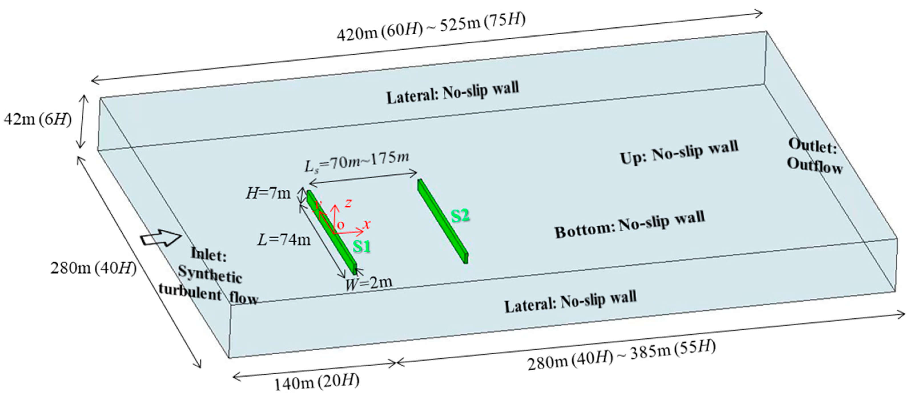
2.3. Domain, Boundaries, and Meshes

Figure 4 shows the considered computational domain together with the adopted boundary conditions. The computational domain is 280 m (40H) wide and 42 m (6H) high, resulting in a maximum blockage ratio of 3.6% among all the shelterbelt models. The length of the computational domain varies from 420 m (60H) to 525 m (75H), depending on the variation in spacing distance between double-arranged shelterbelts. The origin of the along-wind direction (x-axis in Figure 4) is positioned at the leeward edge of the upstream shelterbelt, in accordance with Kurotani et al. (2001) [18]. The distance from the origin to the inlet is 140 m (20H), while the corresponding distance to the outlet ranges between 40H and 55H, depending on the spacing between the double-arranged shelterbelts.

For the inlet boundary, a synthetic turbulent inflow in the atmospheric boundary layer is applied. The time histories generated using the PRFG³ method [34,35] are adopted, and their comparisons with the full-scale results are presented in Section 2.5. An outflow boundary condition is applied at the outlet. No-slip wall conditions are used at the bottom, top and lateral boundaries.

The computational meshes were generated using blockMesh and snappyHexMesh embedded in OpenFOAM. Both coarse and refined meshes were generated for each case to verify the dependence of the results on the adopted grid. Taking as an example the double-arranged shelterbelts with spacing distance L_s = 70 m (10H), an overview of the coarse mesh is presented in Figure 5. The mesh is gradually refined as it approaches the shelterbelt, with cells being bisected at each level of refinement. In the distant region, the mesh features a resolution of 1.5 m in both streamwise (x) and lateral (y) directions. Near the ground, the height of the first cell is 0.65 m, and this height expands vertically (z direction) with a ratio of 1.03. Near the shelterbelt, the mesh dimensions are 0.1875 m in both streamwise (x) and lateral (y) directions, with cell heights ranging from approximately 0.08 to 0.104 m in the canopy region.

2.4. Numerical Setup

Time advancement was carried out using a second-order scheme, with a blending factor of 0.15 for the Euler scheme and 0.85 for the Crank-Nicolson scheme. A time increment $\Delta t$ of 0.1 s was adopted, resulting in a mean Courant number of 0.6 and maximum value of 5, respectively. A centered second-order scheme was employed for the differentiation of diffusive terms, while for the non-linear convection term, the Linear Upwind Stabilized Transport (LUST) scheme was adopted. In particular, the LUST scheme was a fixed blend between the upwind and centered schemes. Blending factors of 0.25 for the upwind scheme and 0.75 for the centered scheme were adopted in this study. The well-known Pressure Implicit with Splitting of Operators (PISO) algorithm was employed for the pressure–velocity coupling. The total runtime for each simulation scenario was 2500 s. The results from the initial 500 s were discarded to eliminate the transient effects. The statistics of the flow field were obtained by averaging over the time window spanning from 500 s to 2500 s.

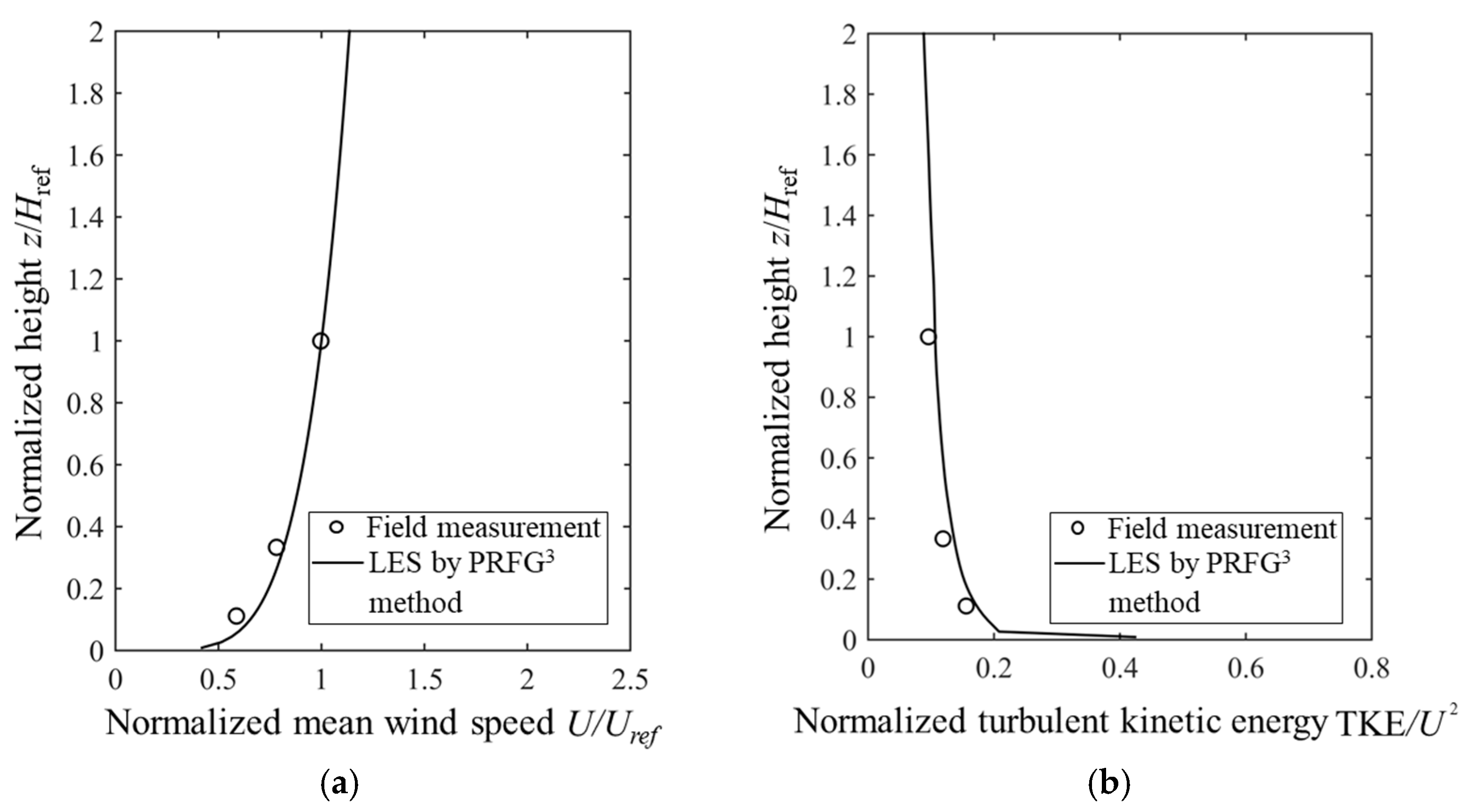
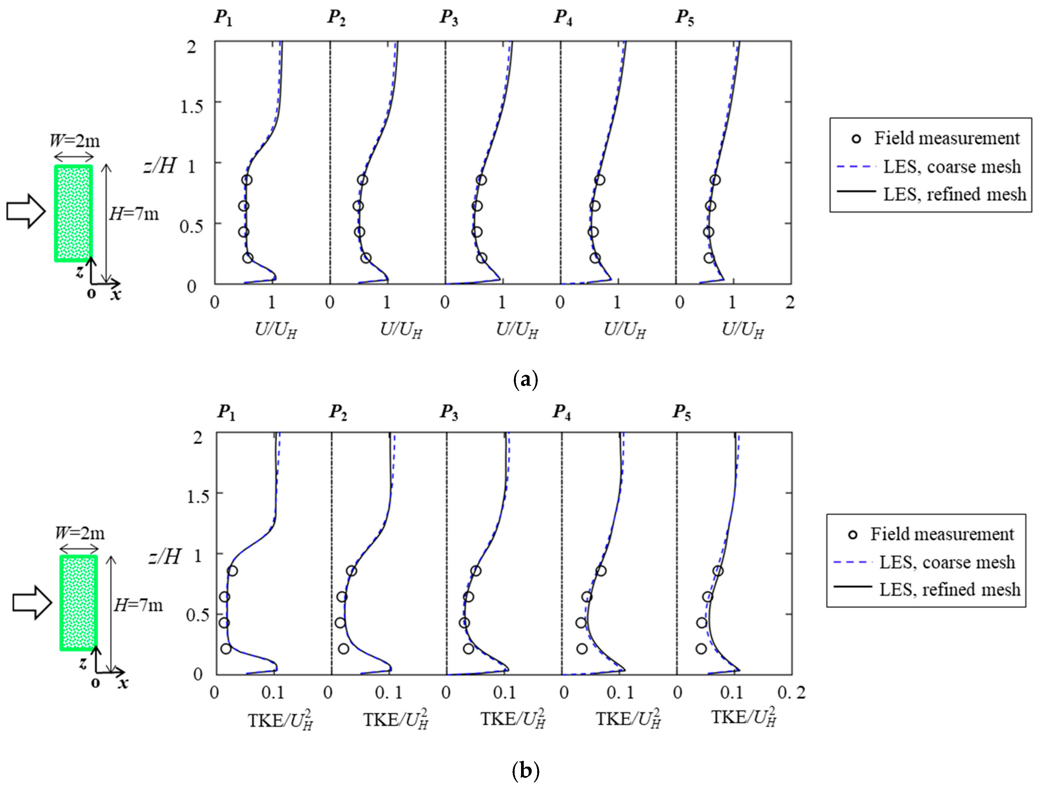
2.5. Validation of Numerical Results

The successful generation of turbulent flow fields in the atmospheric boundary layer was a key step for LES in this study. Figure 6 shows the comparisons of normalized mean wind speed and Turbulent Kinetic Energy, TKE, profiles at the upstream position x/H = −5 obtained from Kurotani et al. (2001) [18] and LES by adopting the PRFG³ synthetic generator. Following Kurotani et al. (2001) [18], a reference height of 9 m, denoted as H_ref, was utilized to normalize the height variable z. Accordingly, the mean wind speed at the reference height denoted by H_ref was used for normalizing wind speed and TKE. As can be seen in Figure 6a,b, the simulated approaching characteristics including mean wind speed and turbulent kinetic energy agree well with the full-sale data.

In order to validate the canopy model adopted in this study, the simulated normalized mean wind speed and TKE in the leeward of the shelterbelt in the vertical plane y/H = 0 were compared with the results of field measurement, as shown in Figure 7. In this case, normalization was performed using the mean wind speed U_H at the height of the shelterbelt z/H = 1 at the location x/H = −5, following the approach of Kurotani et al. (2001) [18]. The results at five particular positions including x/H = 1, 2, 3, 4, and 5 were selected and presented. As shown in Figure 7a, the simulated mean wind speed was consistent with the results obtained from field measurement. Regarding the TKE, as presented in Figure 7b, its values are in good accordance with each other at the upper height, while the numerical results are slightly larger than the reference at lower heights. Overall, the results obtained in the numerical simulations appear to be in good agreement with the field measurements used as reference.

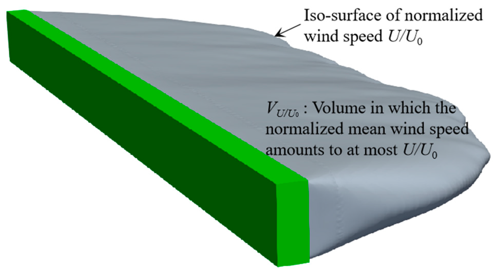
2.6. Definition of Windbreak Effectiveness Indicators

On the basis of normalized mean wind speed U/U₀, three synthetic indicators of shelterbelt effectiveness were defined: protection distance D_U/U0, protection area A_U/U0, and protection volume V_U/U0. These indicators characterize a zone in which the normalized mean wind speed is at most U/U₀, meaning that zones with lower mean wind speeds are included within it. As an example, Figure 8 shows a schematic diagram of the protection volume V_U/U0. Following previous studies [7,36], the protection indicators corresponding to U/U₀ = 0.7, namely D_0.7, A_0.7 and V_0.7, are mainly discussed in this paper. Considering that crops and human activities typically occur at a height of 2 m, this paper focuses on this height when discussing the wind speed distribution in the horizontal direction and the corresponding values of D_0.7 and A_0.7 [37,38].

Furthermore, to quantify the resistance of the shelterbelt to the airflow, the drag coefficient C_d was used, which is calculated as follows:

$$C_d={\displaystyle \frac{F_d}{0.5\rho U_H^{2}A}}$$

(5)

where F_d is the drag force acting on the shelterbelt, ρ is the air density, A is the projected area, and U_H is the referenced mean wind speed for the undisturbed flow (without shelterbelts) at the shelterbelt height H. The mean and fluctuating drag coefficients, denoted by $\overline{C_d}$ and $C_d^{\prime }$, respectively, are mainly discussed in this paper.

3. Results and Discussion

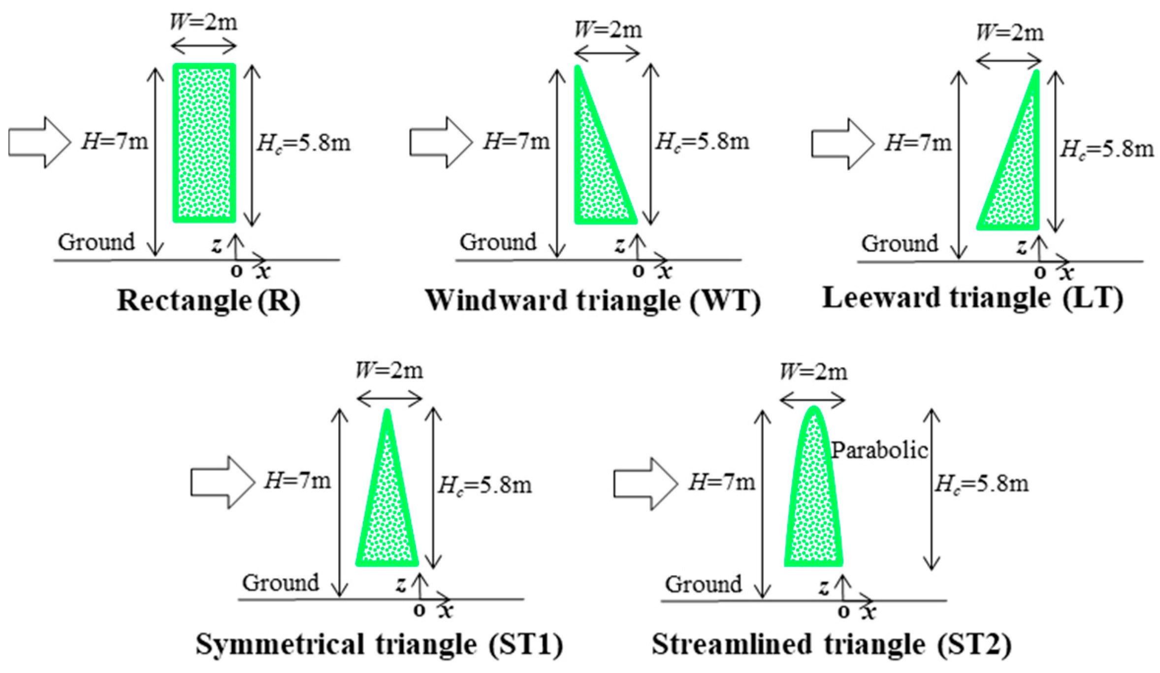
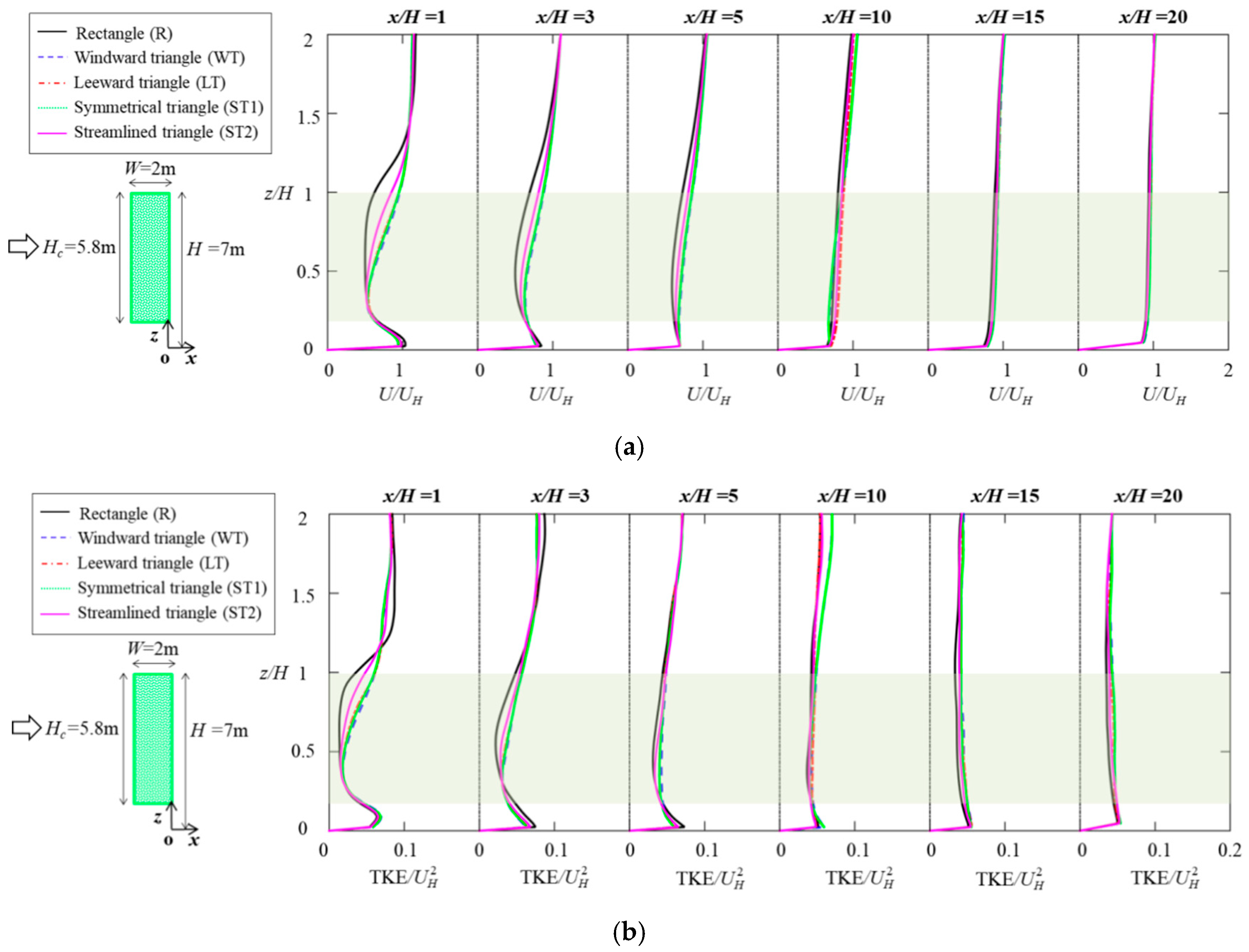
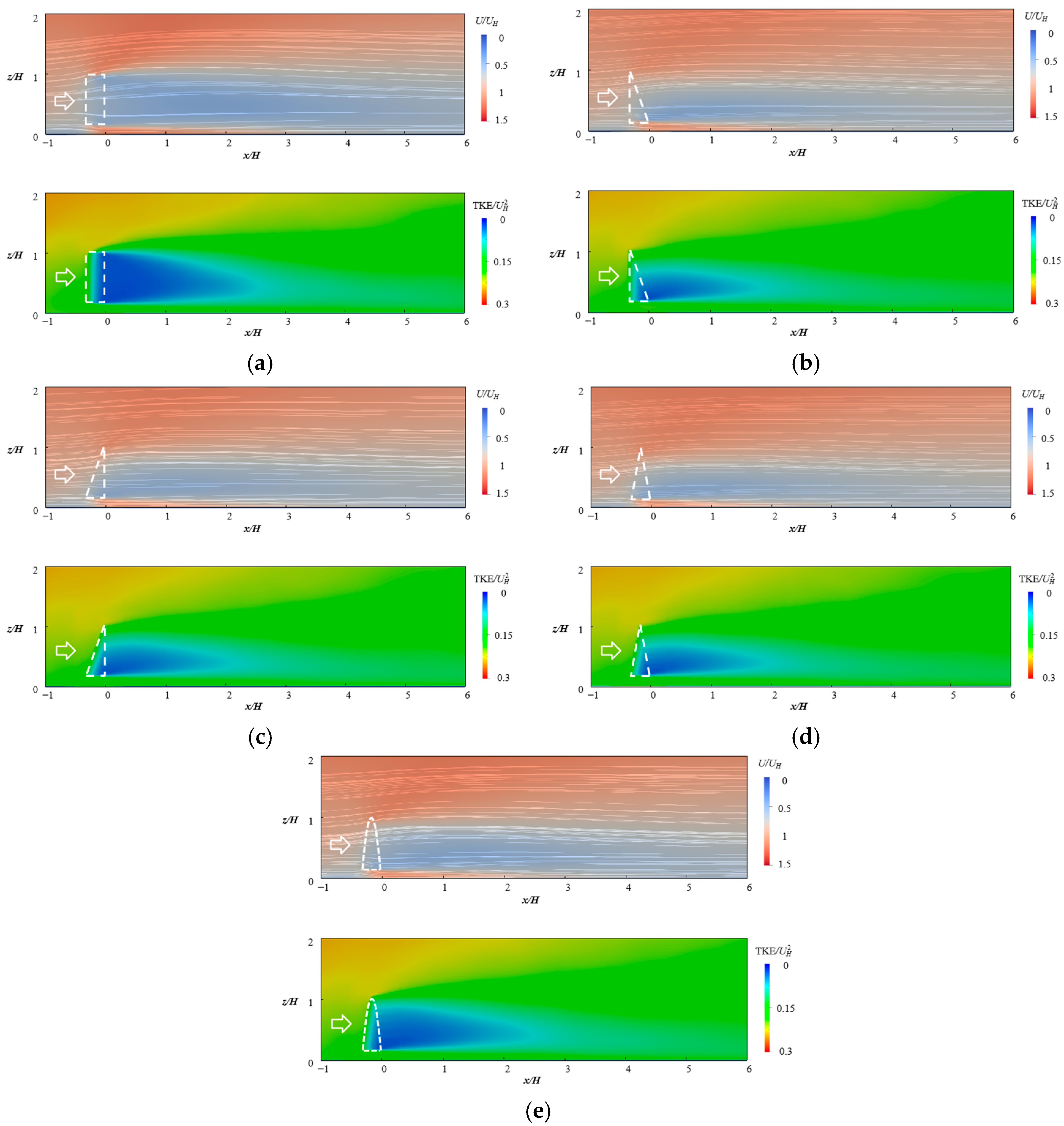
3.1. Effects of Cross-Sectional Shape of Single Shelterbelt

The effects of cross-sectional shape on the flow statistics in the leeward of a single shelterbelt in the vertical plane y/H = 0 are presented in Figure 9. It can be seen that both the mean wind speed and TKE are reduced in the near downstream region of the shelterbelt canopy. Additionally, both the values of mean wind speed and TKE have the largest reductions behind the shelterbelt with an R-shaped cross-section, compared to other shapes, especially in the region with z/H ≥ 0.5 at locations of x/H = 1~3. The shelterbelt with an ST2-shaped cross-section ranks second in mean wind speed and TKE reductions. The corresponding values for shelterbelts with WT-, LT- and ST1-shaped cross-sections are the smallest and exhibit similar values. As the horizontal distance from the leeward edge of the shelterbelt increases, the differences in the statistical characteristics of the flow field between different cross-sectional shapes gradually decrease and tend to become negligible beyond x/H = 10.

Figure 10 presents the distributions of flow statistics in the vertical plane y/H = 0 for different cross-sectional shapes. Similar to Figure 9, the distributions of normalized mean wind speed in Figure 10 show that the wind speed behind the R-shaped cross-sectional shelterbelt decreases significantly, especially in the upper region near the leeward side of the shelterbelt. Comparing the distributions of TKE for different cross-sectional shapes, it can be seen that the R-shaped cross-section has the largest wake area in the leeward region, followed by the ST2-shaped canopy. The shelterbelts with WT-, LT-, and ST1-shaped cross-sections show a smaller wake area. This is consistent with the findings for the mean and fluctuating drag coefficients for shelterbelts with different cross-sectional shapes, as shown in Figure 11. The results indicate that shelterbelts with an R-shaped cross-section exhibit the highest resistance, while those with WT-, LT-, and ST1-shaped cross-sections exhibit the lowest resistance, as expected. These findings align with the wind tunnel studies conducted by Guan et al. (1995) [12] and field tests carried out by Zhu (2008) [8].

Figure 12 shows the horizontal distribution of normalized mean wind speed U/U₀ at a height of z = 2 m. The results indicate that the protection distance and protection area of the R-shaped cross-sectional shelterbelt are the largest. The ST2-shaped cross-sectional shelterbelt follows, while WT-, LT- and ST1-shaped cross-sections exhibit the weakest protection effect. Based on the above results, it is evident that shelterbelts with different canopy shapes but similar canopy volumes result in comparable resistance to airflow, indicating that the canopy volume is the dominating factor which defines the shielding effectiveness. To quantify the windbreak effectiveness of a single shelterbelt with different canopy shapes, the variations in normalized protection distance D_0.7/H, protection area A_0.7/HL, and protection volume V_0.7/HLW with normalized canopy volume V_c/V_R, where V_R represents the canopy volume of an R-shaped shelterbelt with the same height, are plotted in Figure 13. Within the range of parameters considered in this study, the following linear fitting equations between the normalized windbreak indicators and the normalized canopy volume are presented:

$$D_{0.7}/H=6.48V_c/V_R-0.32$$

(6)

$$A_{0.7}/HL=5.58V_c/V_R+1.38$$

(7)

$$V_{0.7}/HLW=20.94V_c/V_R-6.26$$

(8)

3.2. Effects of Canopy Height of a Single Shelterbelt

Figure 14 illustrates the effects of the normalized canopy height H_c/H on the flow statistics behind a single shelterbelt in the vertical plane y/H = 0. As the canopy height increases, the sheltering range, indicated by the reduction in normalized mean wind speed and TKE behind the canopy, expands. The influence of canopy height gradually diminishes below the base of the canopy and near the ground. Furthermore, the differences in the normalized mean wind speed and TKE between different canopy heights gradually decrease proceeding further downstream.

The horizontal variation of the flow statistics around a single shelterbelt with varying canopy heights (vertical plane y/H = 0 at a height of z = 2 m) is shown in Figure 15. For values of normalized canopy height H_c/H equal to 2/7, 3/7, and 4/7, the mean wind speed increases suddenly in close proximity to the leeward edge of the shelterbelt canopy, resulting in a normalized mean wind speed larger than one. This phenomenon is caused by the flow acceleration below the canopy. However, the corresponding mean wind speed shows a rapid decreasing tendency for the normalized canopy heights H_c/H of 5/7, 5.8/7 and 6/7, because the height of z = 2 m is located inside or near the edge of the canopy region. The normalized TKE exhibits a similar tendency to the normalized mean wind speed for different canopy heights.

Figure 16 depicts the variations in the normalized protection volume V_0.7/HLW for a single shelterbelt with different canopy heights. It can be seen that an increase in canopy height results in a gradual increase in the protection volume. The quantitative relationship between the normalized protection volume V_0.7/HLW and the normalized canopy height H_c/H was established through curve fitting as follows:

$${\displaystyle \frac{V_{0.7}}{HLW}}=28.5{\left({\displaystyle \frac{H_c}{H}}\right)}^2-7.1{\displaystyle \frac{H_c}{H}}$$

(9)

As protection distance D_0.7 and protection area A_0.7 at the height of 2 m are null for most canopy heights, their relationship with canopy height is not discussed in this section.

Figure 17 depicts the variations in mean and fluctuating drag coefficient for a single shelterbelt considering different canopy heights (a 2-D rectangular rod and 3-D rectangular plate in uniform smooth flow are also reported for the sake of completeness). It is observed that the changes in mean and fluctuating drag coefficients as a function of the canopy height are not significant. Additionally, taking into account both Figure 16 and Figure 17, it can be concluded that the shelter effects of shelterbelts cannot be inferred based on the drag coefficient alone. This finding is consistent with the Wang and Takle (1997) [10].

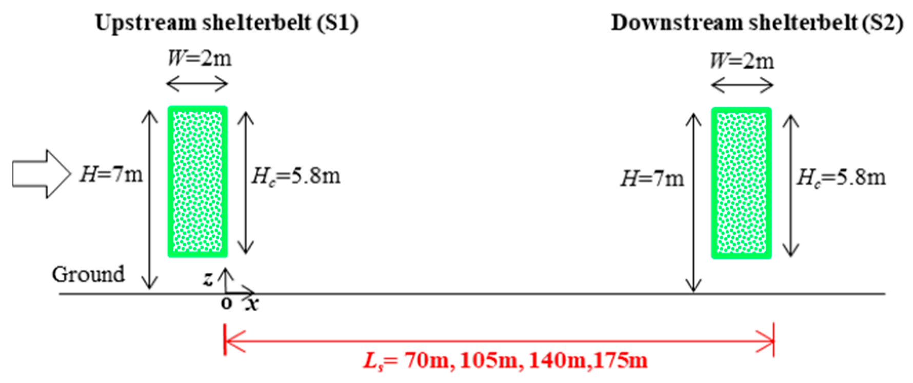
3.3. Effects of Spacing Distance of Double-Arranged Shelterbelts

We now consider double-arranged shelterbelts with a spacing distance of L_s/H = 10. In particular, Figure 18 illustrates the distributions of flow statistics in vertical plane y/H = 0. As expected, the mean wind speed decreases upon encountering the upstream shelterbelt S1. Subsequently, the wind speed gradually recovers after passing through shelterbelt S1 and encounters the second shelterbelt S2, which leads to a second decrease in velocity. The distribution of the turbulent kinetic energy reveals wake regions behind both shelterbelts, with the wake region formed by shelterbelt S2 being larger than that in the downstream region of shelterbelt S1.

Figure 19 reports the impact of different spacing distances on the horizontal variation in normalized mean wind speed and turbulent kinetic energy around double-arranged shelterbelts. The results indicate that, in the case of the double-arranged shelterbelts, values near the shelterbelt S1 are similar to the isolated case. On the contrary, for shelterbelt S2, there is a noticeable and abrupt decrease in both normalized mean wind speed and turbulent kinetic energy, with the magnitude of the decrease in mean wind speed increasing as the spacing distance grows.

To quantify the resistance offered by each shelterbelt to the airflow, Figure 20 shows the influence of the spacing distances on the mean and fluctuating drag coefficients of each shelterbelt within the double-arranged shelterbelts. For shelterbelt S1, the mean and fluctuating drag coefficients exhibit slight variations across different spacing distances, with values similar to those of a single shelterbelt. In contrast, the mean and fluctuating drag coefficients of shelterbelt S2 are lower than those of shelterbelt S1, due to the shielding effect of shelterbelt S1. Notably, the mean drag coefficient of S2, located at a distance of L_s/H = 10, is significantly lower than that of shelterbelt S1, but increases as the spacing distance grows.

To illustrate the impact of spacing distances on the windbreak effectiveness of shelterbelts, Figure 21 shows the horizontal distribution of normalized mean wind speed U/U₀ for double-arranged shelterbelts with examples of spacing distances of L_s/H = 10 and 25 at a height of z = 2 m. The protection distance D_0.7 and protection area A_0.7 are also denoted in the figures. When the downstream shelterbelt S2 is located at 10H from the upstream shelterbelt, the airflow encounters the shelterbelt S2 before it has fully recovered after passing through the shelterbelt S1. As the corresponding spacing distance increases to 25H, the wind speed downstream of shelterbelt S1 is almost completely recovered before encountering the shelterbelt S2. Considering that the drag coefficient of shelterbelt S2 is smaller than that of shelterbelt S2, the corresponding protection region is smaller than that of S1. The variations in the windbreak indicators of shelterbelts S1 and S2 for all the spacing distances considered in this study are shown in Figure 22. When double-arranged shelterbelts have a spacing distance L_s/H = 10, the wind-protected area between them is slightly larger than that of a single shelterbelt. This is due to the interaction between the wake flow of shelterbelt S1 and the shelterbelt S2. This observation is consistent with the findings of Frunk and Ruck [17]. As the spacing distance increases, the protection zone formed by both shelterbelts, S1 and S2, is reduced.

4. Conclusions

A series of LES simulations were carried out to investigate the flow field and windbreak effectiveness around single and double-arranged shelterbelts, focusing on the effects of cross-sectional shape, canopy height, and spacing distance. The following findings were obtained.

(1)

The Darcy–Forchheimer model, which treats the shelterbelt canopy as a porous medium with isotropic properties, appears to provide accurate results, particularly concerning the distributions of mean wind speed and TKE.

(2)

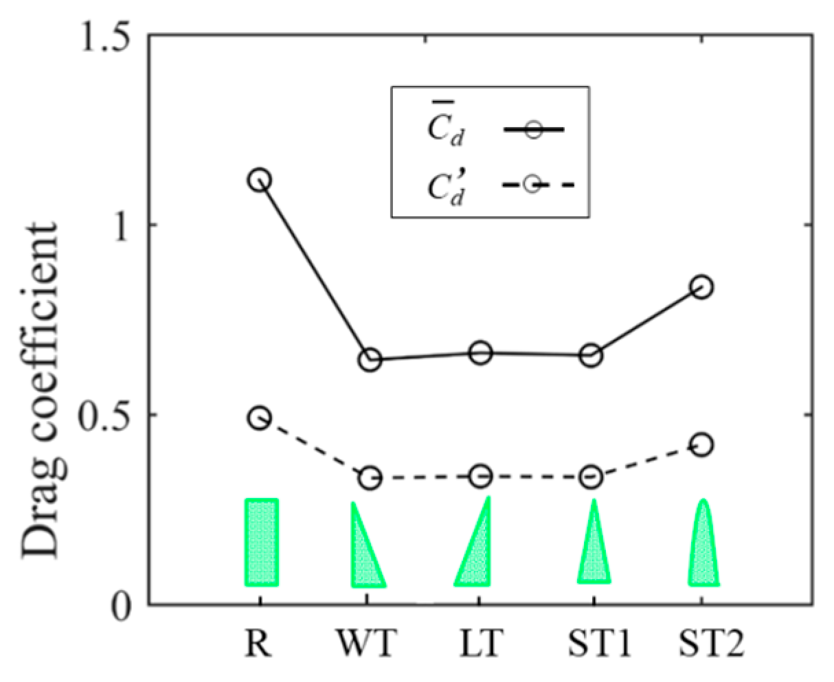
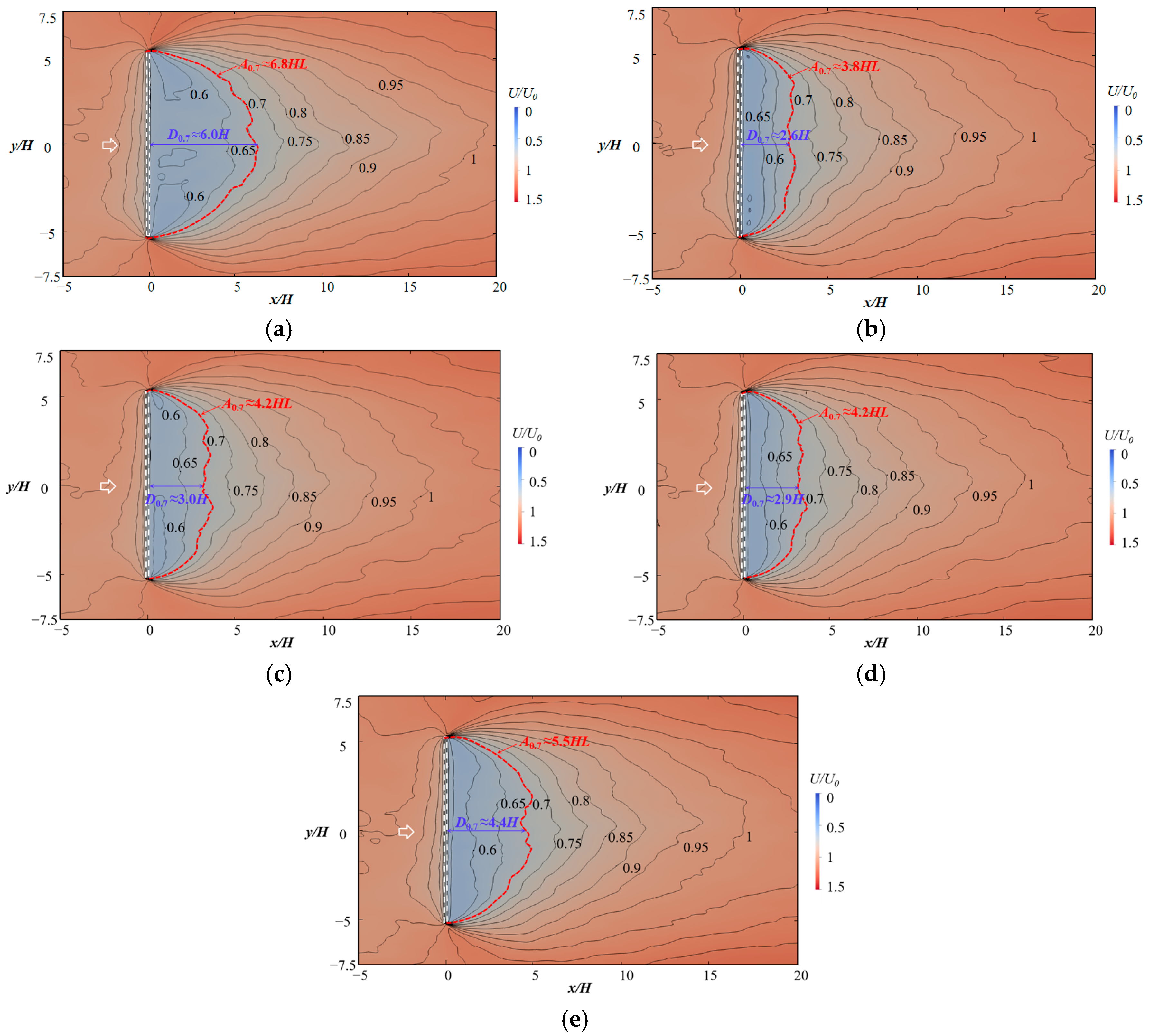
The single shelterbelt with a rectangular-shaped (R-shaped) cross-section exhibits higher resistance and a larger protection region compared to triangular shapes (including the WT, LT, and ST1 shapes) and the streamlined triangular (ST2) shape. The change in canopy volume caused by variation in canopy shape plays the most important role in determining windbreak effectiveness, with the actual shape having a very limited effect.

(3)

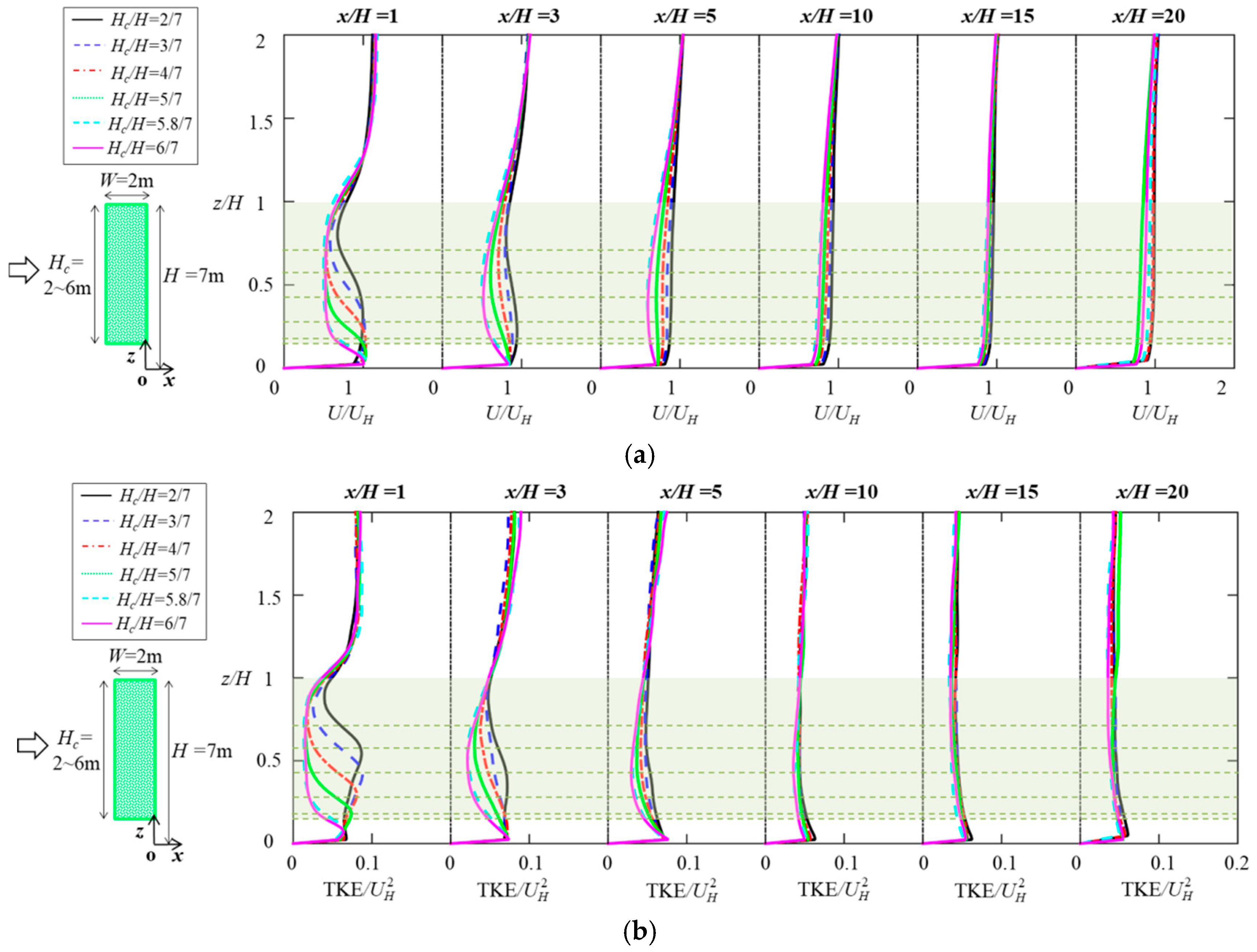
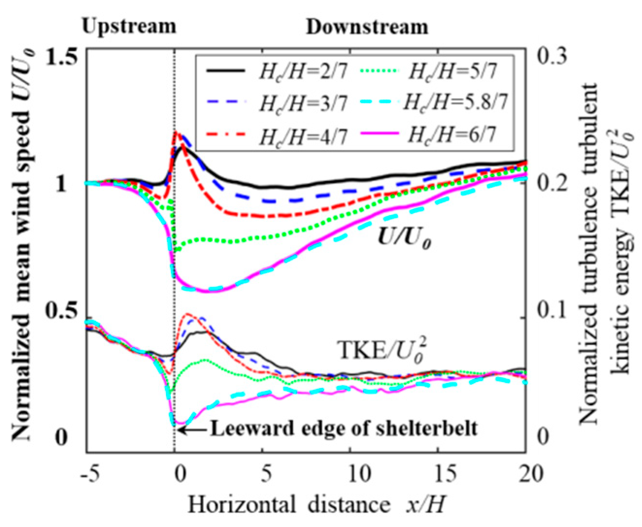
The mean and fluctuating drag coefficients for single shelterbelts with different canopy heights do not show significant differences, indicating that the size effects are less pronounced for porous shelterbelts. However, as expected, a large canopy height results in a larger wind-protection region.

(4)

As the spacing distance of double-arranged shelterbelts increases, the protection zones formed by both shelterbelts are reduced.

References

1. Brandle, J.R.; Hodges, L.; Zhou, X.H. Windbreaks in North American agricultural systems. Agroforest. Syst. 2004, 61, 65–78. [Google Scholar]
2. Li, M.; Liu, A.; Zou, C.; Xu, W.; Shimizu, H.; Wang, K. An overview of the “Three-North” Shelterbelt project in China. For. Stud. China. 2012, 14, 70–79. [Google Scholar] [CrossRef]
3. Mohammed, A.E.; Stigter, C.J.; Adam, H.S. On shelterbelt design for combating sand invasion. Agr. Ecosyst. Environ. 1996, 57, 81–90. [Google Scholar] [CrossRef]
4. Su, Z.; Zhou, T.; Zhang, X.; Wang, X.; Wang, J.; Zhou, M.; Zhang, J.; He, Z.; Zhang, R. A preliminary study of the impacts of shelter forest on soil erosion in cultivated land: Evidence from integrated 137Cs and 210Pbex measurements. Soil Till. Res. 2021, 206, 104843. [Google Scholar] [CrossRef]
5. Wang, H.; Zhou, H. A simulation study on the eco-environmental effects of 3N Shelterbelt in North China. Glob. Planet. Change. 2003, 37, 231–246. [Google Scholar]
6. Zhu, J.J.; Zheng, X.; Yan, Q.L. Assessment of Impacts of the Three-North Protective Forest Program on Ecological Environments by Remote Sensing Technology—Launched after 30 Years (1978–2008); Science Press: Beijing, China, 2016. (In Chinese) [Google Scholar]
7. Zhou, X.H.; Brandle, J.R.; Mize, C.W.; Takle, E.S. Three-dimensional aerodynamic structure of a tree shelterbelt: Definition, characterization and working models. Agroforest. Syst. 2004, 63, 133–147. [Google Scholar] [CrossRef]
8. Zhu, J.J. Wind shelterbelts. In Encyclopedia of Ecology; Fath, B.D., Ed.; Academic Press: Oxford, UK, 2008; pp. 38303–38312. [Google Scholar]
9. Wang, J.; Patruno, L.; Zhao, G.; Tamura, Y. Windbreak effectiveness of shelterbelts with different characteristic parameters and arrangements by means of CFD simulation. Agric. For. Meteorol. 2024, 344, 109813. [Google Scholar] [CrossRef]
10. Wang, H.; Takle, E.S. Model-simulated influences of shelterbelt shape on wind-sheltering efficiency. J. Appl. Meteorol. 1997, 36, 695–704. [Google Scholar] [CrossRef]
11. Woodruff, N.P.; Zingg, A.W. Wind tunnel studies of shelterbelt models. J. For. 1953, 53, 173–178. [Google Scholar]
12. Guan, D.; Wang, S.; Zhu, T. Experimental study on the relationship between section form of shelterbelt and its wind resistance. Chinse J. Ecol. 1995, 14, 15–19. (In Chinese) [Google Scholar]
13. Cao, X. Farmland Shelterbelt Science; China Forestry Publishing House: Beijing, China, 1983. [Google Scholar]
14. Zhu, J.J. A review of the present situation and future prospect of science of protective forest. Chinese J. Plant. Ecol. 2013, 37, 872–888. (In Chinese) [Google Scholar] [CrossRef]
15. Sun, Q.; Zheng, B.; Liu, T.; Zhu, L.; Hao, X.; Han, Z. The optimal spacing interval between principal shelterbelts of the farm-shelter forest network. Environ. Sci. Pollut. Res. 2022, 29, 12680–12693. [Google Scholar] [CrossRef]
16. Woodruff, N.P. The spacing interval for supplemental shelterbelts. J. For. 1956, 54, 115–122. [Google Scholar]
17. Frank, C.; Ruck, B. Double-arranged mound-mounted shelterbelts: Influence of porosity on wind reduction between the shelters. Environ. Fluid Mech. 2005, 5, 267–292. [Google Scholar] [CrossRef]
18. Kurotani, Y.; Kiyota, N.; Kobayashi, S. Windbreak effect of tsuijimatsu in Izumo: Part 2. In Summaries of Technical Papers of Annual Meeting; Architectural Institute of Japan: Tokyo, Japan, September 2001; pp. 745–746. (In Japanese) [Google Scholar]
19. Zhao, W.; Hu, G.; Zhang, Z.; He, Z. Shielding effect of oasis-protection systems composed of various forms of wind break on sand fixation in an arid region: A case study in the Hexi Corridor, northwest China. Ecol. Eng. 2008, 33, 119–125. [Google Scholar] [CrossRef]
20. Rudnicki, M.; Mitchell, S.J.; Novak, M.D. Wind tunnel measurements of crown streamlining and drag relationships for three conifer species. Can. J. For. Res. 2004, 34, 666–676. [Google Scholar] [CrossRef]
21. Cao, J.; Tamura, Y.; Yoshida, A. Wind tunnel study on aerodynamic characteristics of shrubby specimens of three tree species. Urban For. Urban Green. 2012, 11, 465–476. [Google Scholar] [CrossRef]
22. Ferreira, A.D. Structural design of a natural windbreak using computational and experimental modeling. Environ. Fluid Mech. 2011, 11, 517–530. [Google Scholar] [CrossRef]
23. Amorim, J.H.; Rodrigues, V.; Tavares, R.; Valente, J.; Borrego, C. CFD modelling of the aerodynamic effect of trees on urban air pollution dispersion. Sci. Total Environ. 2013, 461–462, 541–551. [Google Scholar] [CrossRef] [PubMed]
24. Qi, Y.; Ishihara, T. Numerical study of turbulent flow fields around a row of trees and an isolated building by using modified k-ε model and LES model. J. Wind. Eng. Ind. Aerod. 2018, 177, 293–305. [Google Scholar] [CrossRef]
25. Wang, Y.; Zeng, X.; Decker, J.; Dawson, L. A GPU-Implemented Lattice Boltzmann Model for Large Eddy Simulation of Turbulent Flows in and around Forest Shelterbelts. Atmosphere 2024, 15, 735. [Google Scholar] [CrossRef]
26. Kadaverugu, R.; Purohit, V.; Matli, C.; Biniwale, R. Improving accuracy in simulation of urban wind flows by dynamic downscaling WRF with OpenFOAM. Urban Clim. 2021, 38, 100912. [Google Scholar] [CrossRef]
27. Mochida, A.; Tabata, Y.; Iwata, T.; Yoshino, H. Examining tree canopy models for CFD prediction of wind environment at pedestrian level. J. Wind. Eng. Ind. Aerod. 2008, 96, 1667–1677. [Google Scholar] [CrossRef]
28. Bitog, J.P.; Lee, I.; Hwang, H.; Shin, M.; Hong, S.; Seo, I.; Kwon, K.; Mostafa, E.; Pang, Z. Numerical simulation study of a tree windbreak. Biosyst. Eng. 2012, 111, 40–48. [Google Scholar] [CrossRef]
29. Yan, C.; Huang, W.; Miao, S.; Cui, G.; Zhang, Z. Large-eddy simulation of flow over a vegetation-like canopy modelled as arrays of bluff-body elements. Bound-Lay. Meteorol. 2017, 165, 233–249. [Google Scholar] [CrossRef]
30. Maruyama, T. Large eddy simulation of turbulent flow around a windbreak. J. Wind. Eng. Ind. Aerod. 2008, 96, 1998–2006. [Google Scholar] [CrossRef]
31. Smagorinsky, J. General circulation experiments with the primitive equations: I. The basic experiment. Mon. Weather Rev. 1963, 91, 99–164. [Google Scholar] [CrossRef]
32. Rosenfeld, M.; Marom, G.; Bitan, A. Numerical simulation of the airflow across trees in a windbreak. Bound. Layer Meteorol. 2010, 135, 89–107. [Google Scholar] [CrossRef]
33. Liu, C.; Zheng, Z.; Cheng, H.; Zou, X. Airflow around single and multiple plants. Agric. For. Meteorol. 2018, 252, 27–38. [Google Scholar] [CrossRef]
34. Patruno, L.; Ricci, M. A systematic approach to the generation of synthetic turbulence using spectral methods. Comput. Method. Appl. Meteorol. 2018, 340, 881–904. [Google Scholar] [CrossRef]
35. Bervida, M.; Patruno, L.; Stanič, S.; de Miranda, S. Synthetic generation of the atmospheric boundary layer for wind loading assessment using spectral methods. J. Wind. Eng. Ind. Aerod. 2020, 196, 104040. [Google Scholar] [CrossRef]
36. Torita, H.; Satou, H. Relationship between shelterbelt structure and mean wind reduction. Agric. For. Meteorol. 2007, 145, 186–194. [Google Scholar] [CrossRef]
37. Liu, B.; Qu, J.; Zhang, W.; Tan, L.; Gao, Y. Numerical evaluation of the scale problem on the wind flow of a windbreak. Sci. Rep. 2014, 4, 6619. [Google Scholar] [CrossRef] [PubMed]
38. Sai, K.; Zhao, Y.; Bao, Y.; Liu, C.; Ding, G.; Gao, G. Wind-tunnel tests study of shelter effects of deciduous farmland shelterbelts in arid and semi-arid areas. Trans. CSAE 2021, 37, 157–165. (In Chinese) [Google Scholar]
Figure 1. Variations in cross-sectional shapes of single shelterbelt (Case I).
Forests 15 01760 g001
Figure 2. Variations in canopy heights of single shelterbelt (Case II).
Forests 15 01760 g002
Figure 3. Variations in spacing distances between double-arranged shelterbelts (Case III).
Forests 15 01760 g003
Figure 4. Domain and adopted boundaries.
Forests 15 01760 g004
Figure 5. Overview of the coarse computational mesh with the double-arranged shelterbelts with spacing distance Ls = 70 m (10H).
Forests 15 01760 g005
Figure 6. Comparison of approaching flow characteristics at the upstream position x/H = −5 obtained by LES and field measurement. (a) Normalized mean wind speed. (b) Normalized TKE.
Forests 15 01760 g006
Figure 7. Comparison of flow statistics in leeward of shelterbelt obtained by LES and field measurement. (a) Normalized mean wind speed. (b) Normalized TKE.
Forests 15 01760 g007
Figure 8. Schematic diagram of protection volume.
Forests 15 01760 g008
Figure 9. Flow statistics in the leeward of a single shelterbelt with different cross-sectional shapes in vertical plane y/H = 0. (a) Normalized mean wind speed. (b) Normalized TKE.
Forests 15 01760 g009
Figure 10. Distributions of flow statistics for a single shelterbelt with different cross-sectional shapes in vertical plane y/H = 0. (a) Rectangle (R); (b) windward triangle (WT); (c) leeward triangle (LT); (d) symmetrical triangle (ST1); (e) streamlined triangle (ST2).
Forests 15 01760 g010
Figure 11. Variations in mean and fluctuating drag coefficient for a single shelterbelt with different cross-sectional shapes.
Forests 15 01760 g011
Figure 12. Distribution of normalized mean wind speed U/U0 for a single shelterbelt with different cross-sectional shapes in horizontal plane with z = 2 m. (a) Rectangle (R). (b) Windward triangle (WT). (c) Leeward triangle (LT). (d) Symmetrical triangle (ST1). (e) Streamlined triangle (ST2).
Forests 15 01760 g012
Figure 13. Variations in normalized protection distance D0.7/H, protection area A0.7/HL, and protection volume V0.7/HLW for a single shelterbelt with different cross-sectional shapes.
Forests 15 01760 g013
Figure 14. Flow statistics in the leeward of a single shelterbelt with different canopy heights in vertical plane y/H = 0. (a) Normalized mean wind speed. (b) Normalized TKE.
Forests 15 01760 g014
Figure 15. Horizontal variation in flow statistics around a single shelterbelt with different canopy heights in vertical plane y/H = 0 at height of z = 2 m.
Forests 15 01760 g015
Figure 16. Variations in normalized protection volume V0.7/HLW for a single shelterbelt with different canopy heights.
Forests 15 01760 g016
Figure 17. Variations in mean and fluctuating drag coefficient for a single shelterbelt with different canopy heights. (a) Comparison with 2-D rectangular rod. (b) Comparison with 3-D rectangular plate.
Forests 15 01760 g017
Figure 18. Distributions of flow statistics of double-arranged shelterbelts with spacing distance of Ls/H = 10 in vertical plane y/H = 0.
Forests 15 01760 g018
Figure 19. Horizontal variations in flow statistics around double-arranged shelterbelts with different spacing distances in vertical plane y/H = 0 at height of z = 2 m.
Forests 15 01760 g019
Figure 20. Variations in mean and fluctuating drag coefficient of double-arranged shelterbelts with different spacing distances.
Forests 15 01760 g020
Figure 21. Horizontal distribution of normalized mean wind speed U/U0 for double-arranged shelterbelts with spacing distances of Ls/H = 10 and 25 at height of z = 2 m. (a) Ls/H = 10, (b) Ls/H = 25.
Forests 15 01760 g021
Figure 22. Variations of normalized protection distance D0.7/H, protection area A0.7/HL, and protection volume V0.7/HLW for double-arranged shelterbelts with different spacing distances.
Forests 15 01760 g022