Abstract
Accurate regional carbon sequestration estimates are essential for China’s emission reduction and carbon sink enhancement efforts to address climate change. Enhancing the spatial precision of vegetation carbon sink estimates is crucial for a deeper understanding of the underlying response mechanisms, yet this remains a significant challenge. In this study, the Beijing–Tianjin–Hebei (BTH) region was selected as the study area. We employed the GF-SG (Gap filling and Savitzky–Golay filtering) model to fuse Landsat and MODIS data, generating high-resolution imagery to enhance the accuracy of NPP (Net Primary Productivity) and NEP (Net Ecosystem Productivity) estimates for this region. Subsequently, the Sen+MK model was used to analyze the spatiotemporal variations in carbon sinks. Finally, the land use intensity index, which reflects human activity disturbances, was applied, and the bivariate Moran’s spatial autocorrelation method was used to analyze the response mechanisms of carbon sinks. The results indicate that the fused GF-SG NDVI (Normalized Difference Vegetation Index) data provided highly accurate 30 m resolution imagery for estimating NPP and NEP. The spatial distribution of carbon sinks in the study area showed higher values in the northeastern forest regions, relatively high values in the southeastern plains, and lower values in the northwestern plateau and central urban areas. Additionally, 58.71% of the area exhibited an increasing trend, with 11.73% showing significant or strongly significant growth. A generally negative spatial correlation was observed between land use intensity and carbon sinks, with the impact of land use intensity on carbon sinks exceeding 0.3 in 2010. This study provides methodological insights for obtaining vegetation monitoring data and estimating carbon sinks in large urban agglomerations and offers scientific support for developing ecological and carbon reduction strategies in the BTH region.
1. Introduction
Vegetation plays a crucial role in terrestrial ecosystems as a carbon sink, absorbing and sequestering carbon through photosynthesis [1,2,3]. This process effectively slows the rise in atmospheric CO₂ concentrations and mitigates global warming, providing an essential pathway toward achieving carbon neutrality [4,5,6]. Two indicators—Net Primary Productivity (NPP) and Net Ecosystem Productivity (NEP)—reflect the net carbon exchange in terrestrial ecosystems and are commonly used to measure the size of carbon sinks. Therefore, an in-depth exploration of the processes and results of NPP and NEP estimation is vital for assessing regional ecological changes and carbon sink capacity. As a critical strategic development region in China, the Beijing–Tianjin–Hebei (BTH) area has a forest coverage rate of approximately 35%. The region’s carbon sink capacity is considered a key indicator for assessing the comprehensive development and coordinated growth of this urban cluster. However, current assessments of the region’s carbon sink capacity based on publicly available NPP and NEP data are limited by low accuracy. For example, the resolution of the MOD17A3 NPP data product is 1 km [7], and most studies in this region use NPP and NEP data with spatial resolutions of 500 m or higher [8,9]. Therefore, obtaining high-resolution spatial data on NPP and NEP for the BTH region is critical for accurate estimation of the region’s carbon sink capacity and for further research into the factors influencing carbon sinks and their response mechanisms.
Among the models used to estimate vegetation NPP and NEP, remote sensing-based methods are the most widely applied and well-developed. The key to obtaining high-resolution NPP and NEP data lies in acquiring effective high-resolution remote sensing imagery. MODIS data, which are commonly used for NPP and NEP estimation, just have a spatial resolution of 500 m. Landsat satellite imagery offers a resolution of 30 m, which can enhance the accuracy of NPP and NEP estimation. However, due to cloud cover, Landsat imagery often has gaps. To address this issue, the MODIS–Landsat NDVI spatiotemporal fusion technique has emerged in recent years. This technique integrates MODIS and Landsat data, allowing for the reconstruction of NDVI data with higher spatiotemporal resolution [10,11]. This method helps overcome the problem of cloud obstruction by using multiple base images to generate a fused image, with the final fused image derived from the weighted averages of multiple fusion estimates. Chen et al. [12] further addressed the time-consuming nature of processing multiple base images by proposing the GF-SG algorithm, based on MODIS–Landsat data fusion, which has proven effective in various challenging scenarios [12]. The GF-SG method is a robust reconstruction technique that is less sensitive to cloud detection errors. It effectively utilizes continuous MODIS NDVI time series data to generate Landsat NDVI time series data and can be applied to large-scale regional studies.
Currently, remote sensing-based vegetation NPP and NEP simulation models fall into three main categories: climate productivity models, light-use efficiency models, and vegetation physiological–ecological process models [13]. Among these, the CASA model (Carnegie–Ames–Stanford Approach) [14] is the most widely used [15,16,17]. This model can be adapted for NPP and NEP estimation at regional or global scales across different ecosystems and climate types [18]. To meet the needs of specific studies, the CASA model has undergone further improvements. Zhu et al. [19] incorporated vegetation cover classification data into the model, accounting for the impact of classification accuracy on NPP estimation. Using the principle of minimizing error and actual NPP measurements in China, he simulated the maximum light-use efficiency for different vegetation types, aligning the model more closely with China’s conditions. Additionally, he incorporated meteorological data—such as temperature, precipitation, and net solar radiation—along with a regional evapotranspiration model to estimate water stress factors, thereby ensuring the reliability and availability of data while simplifying parameters to enhance the model’s practical applicability. Liu et al. [20] improved the CASA model by introducing new methods to estimate the fraction of absorbed photosynthetically active radiation (FPAR) and the water stress coefficient (WSC), which improved NPP estimation accuracy by 8.1% over the original model. Qiu [21] optimized the estimation of optimal temperature and maximum light-use efficiency to calculate NEP in European terrestrial ecosystems, increasing NEP from 0.252 to 0.428 and reducing RMSE (Root Mean Square Error) from 84.557 to 63.720 gC·m−2·month−1. In this study, we used the CASA model modified by Zhu et al. [19], which has been adapted to China’s vegetation distribution characteristics and is suitable for simulating NPP and NEP in the BTH region.
Analyzing the response mechanisms of carbon sinks is crucial for formulating future environmental policies, maintaining regional ecological sustainability, and ensuring pathways to enhance carbon sinks while reducing emissions. Among the many influencing factors, human activity is a major disturbance that reduces the productivity of terrestrial ecosystems and significantly impacts regional carbon sinks [22]. Since China’s reform and opening-up, urbanization has accelerated, increasing urban populations and inevitably causing significant ecological damage, which in turn affects carbon sink capacity. However, within the vast BTH region, human activity-related data are difficult to obtain, and studies on the spatial heterogeneity of the impact of human activities on carbon sinks are still lacking.
In this study, we use land use intensity as an indicator to analyze carbon sink responses. Land use intensity, calculated from multi-temporal land cover data, represents the degree of ecological disturbance caused by different land use types [23]. By incorporating the impact of human activities on land use intensity, this indicator directly reflects the extent and depth of land utilization, indirectly representing the degree of ecological disturbance caused by human activities [24]. Moreover, this indicator is straightforward to calculate. Among the various methods for analyzing the impact of land use intensity, the bivariate Moran’s I index is commonly used to assess the spatial correlation between two variables and has been widely applied in spatial analysis and geographic data modeling. Bivariate spatial autocorrelation considers the interaction between two variables within the same spatial unit, using a spatial weighting matrix to compare the spatial distribution of one variable with that of another based on proximity [25]. Additionally, the bivariate LISA (Local Indicators of Spatial Association) method helps reveal the underlying processes and mechanisms of development. Bivariate LISA statistics, as a local Moran’s I index, have been successfully applied in various fields, such as exploring the spatial relationships between wildfire risk and social vulnerability, urban housing and urban heat islands, and water scarcity and water use efficiency [26]. Therefore, this study combines the bivariate Moran’s I spatial autocorrelation analysis and bivariate LISA statistics to examine the spatial correlation characteristics and dynamic evolution trends of NEP and land use intensity in the study area.
In summary, this study aimed to enhance the accuracy of remote sensing for NPP and NEP and further identify the mechanisms by which land use intensity influences carbon sequestration. First, it used the GF-SG method to fuse Landsat and MODIS NDVI data, establishing a high-precision NDVI dataset. Then, using the CASA model, we estimated the NPP and NEP of the study area and analyzed the spatiotemporal changes using the Sen+MK trend analysis method. Finally, the land use intensity index was calculated, and its spatial heterogeneity with NEP was explored. This research provides essential baseline carbon sink data for studying forest carbon cycles in the region and clarifies the mechanisms by which land use intensity affects the spatiotemporal distribution of carbon sinks. The findings will provide decision-making support for ecological construction and carbon sequestration strategies in the BTH megacity region.
2. Materials and Methods
2.1. Study Site
The study area is the Beijing–Tianjin–Hebei (BTH) urban agglomeration, which includes Beijing, Tianjin, and 11 prefecture-level cities under the jurisdiction of Hebei Province. These cities are Shijiazhuang, Handan, Xingtai, Baoding, Zhangjiakou, Chengde, Tangshan, Qinhuangdao, Cangzhou, Hengshui, and Langfang, covering a total area of approximately 218,000 km². The region is located between longitudes 113°27′ E to 119°50′ E and latitudes 36°05′ N to 42°40′ N, as shown in Figure 1.
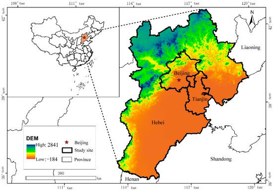
Figure 1.
Geographical location of research area.
The BTH region is the largest urban cluster in northern China. However, as a key area for national strategic development, its rapid urbanization and significant population growth have had a profound impact on forest ecosystems and carbon sequestration capacity. Over the years, the continuous expansion of urban areas has led to forest shrinkage and degradation. In recent years, large-scale afforestation initiatives have been implemented in major cities across the BTH plain to restore forest ecosystems. From 2000 to 2020, noticeable changes in forest cover occurred in the region, highlighting the urgent need to investigate and understand the changes in carbon sequestration capacity and the spatiotemporal mechanisms influenced by human activities.
2.2. Data Sources
Remote Sensing Data: This study integrated NDVI and MODIS remote sensing data from 2000 to 2020, resulting in output data with a temporal resolution of 8 days and a spatial resolution of 30 m. The MODIS dataset used was MOD09Q1, while the Landsat data included the processed products from Landsat 8 (LANDSAT/LC08/C02/T1_L2) and Landsat 5 (LANDSAT/LT05/C02/T1_L2). Both datasets were sourced from https://code.earthengine.google.com/ (accessed on 10 January 2024).
Land Cover Data: The land cover data were obtained from the 1985–2020 global 30 m fine surface cover dynamic monitoring products released by the Aerospace Information Research Institute of the Chinese Academy of Sciences on the Big Earth Data Science and Engineering website. The dataset was based on the latest 2020 Global 30 m Fine Classification Surface Cover Product (GLC_FCS30-2020).
Meteorological Data: Temperature and precipitation data from 2000 to 2020 for this study were sourced from the National Climatic Data Center (NCDC) of the United States. The dataset includes temperature and precipitation records from 27 meteorological stations within the BTH region and surrounding areas. Solar radiation data used the daily average solar radiation dataset (1961–2010) from the Institute of Tibetan Plateau Research and sunshine duration data from the China Meteorological Data Service Center (2000–2020).
National Forest Inventory Data: To validate the NPP estimation results obtained using the CASA model, this study utilized National Forest Inventory data provided by the National Forestry and Grassland Administration. This dataset is based on detailed forest surveys conducted at the stand level, organized by the national authority. These surveys are typically carried out every 10 years, with key provinces and cities surveyed every 5 years. The NPP calculated from this dataset is used as the ground truth datum in this study.
2.3. Methodologies
2.3.1. NDVI Fusion Based on the GF-SG Model
The GF-SG model was primarily used to reconstruct high-quality, continuous Landsat NDVI time series data for the study area, providing input for the subsequent CASA model. This process involved two steps: (1) Gap Filling Stage: This step fills gaps in the original Landsat NDVI time series data, generating a synthetic MODIS–Landsat NDVI time series. (2) Noise Reduction: An integrated weighted Savitzky–Golay (SG) filter was applied to reduce residual noise in the synthetic time series.
During the gap-filling stage, the correlation coefficient between the interpolated MODIS NDVI pixel values and the cloud-free Landsat observations for each target pixel was calculated. This determined similar pixels within a local adjacent window (40 × 40 pixels, approximately 1.2 × 1.2 km) for each target pixel. In this study, we considered adjacent pixels with a correlation coefficient greater than 0.8 to be similar pixels for the target pixel , which could then be used to generate NDVI values for the target pixel.
where is the number of similar pixels, is the weight of the -th similar pixel, determined by the similarity between the time series data of the target pixel and that of the similar pixel, quantified by their correlation coefficient.
To account for systematic errors in NDVI values from Landsat and MODIS data (e.g., differences in spectral response functions), the GF-SG model used a linear transformation formula [27] and applied a linear transfer function to adjust .
where and are the slope and intercept of the linear model, represents the adjusted MODIS NDVI time series data.
2.3.2. Carbon Sink Estimation Based on the CASA Model
(1) NPP EstimationThe CASA model (Carnegie–Ames–Stanford Approach) is one of the most widely used models for simulating vegetation NPP and NEP using remote sensing data. It is highly adaptable for estimating NPP and NEP at regional or global scales across various ecosystems and climate types. The CASA model is a light-use efficiency model that calculates NPP by multiplying the absorbed photosynthetically active radiation (APAR) by the light-use efficiency of converting APAR into plant biomass. This study utilized a modified CASA model, improved by Zhu et al. [19], which was adapted for the characteristics of China’s vegetation distribution. The model was applied to estimate NPP in the BTH region for the years 2001, 2005, 2010, 2015, and 2020.
The calculation formula is as follows:
where represents the pixel, represents time, is the net primary productivity of pixel in month (unit: g/m²), is the actual light-use efficiency of pixel in month (unit: g/mJ), is the absorbed photosynthetically active radiation (unit: mJ/m²).
where the constant represents the proportion of total solar radiation usable by vegetation for photosynthesis, is the total solar radiation, is the fraction of photosynthetically active radiation absorbed by vegetation, which can be estimated using NDVI data [19].
where represents the limitations on light-use efficiency due to extreme low or high temperatures, represents the environmental temperature, represents the impact of water availability on light-use efficiency, is the maximum light-use efficiency under ideal conditions.
The inputs for the CASA model include land cover data, meteorological data (temperature, precipitation, solar radiation), NDVI data, vegetation type data, and static parameter files derived from NDVI maxima and vegetation type. The static parameters, including maximum light-use efficiency, NDVImin, and SRmin (the minimum SR value, which is the ratio of near-infrared reflectance to red light reflectance, is used to analyze the health status of vegetation), used in this study were consistent with the findings of Zhu et al. [19], as shown in Table 1.

Table 1.
Parameters of the CASA model including maximum light energy utilization, NDVImin, and SRmin.
(2) Validation of NPP Estimation Results
To ensure the accuracy of the NPP estimation in this study, we employed direct validation methods. We collected data from China’s 7th to 9th National Forest Inventory to calculate the actual NPP values. These forest inventories in the BTH region were conducted in 2006, 2011, and 2016. Since the annual NPP differences are relatively small, we used the data from these inventories to validate the NPP estimates produced by the CASA model for 2005, 2010, and 2015. The validation was conducted in two steps: First, we calculated the biomass density using the conversion formula between stand volume and biomass (Equations (3)–(7)). Then, we calculated NPP based on the relationship between biomass and NPP (Equations (3)–(8)). The calculated NPP values were used to validate our model results by comparing correlation coefficients, MAPE, and RMSE for accuracy.
where represents the biomass density (mg/ha) for tree species , is the stand volume (m³/ha), and are the slope and intercept for each tree species. Further details can be found in the studies of Qiu [28] and Liang et al. [29]. In the second equation, is the biomass per unit area, is the stand age, and and are constants specific to the tree species. Additional information is available in the works of Liu and Wang [30] and Wang et al. [31].
(3) NEP Estimation
Net Ecosystem Productivity (NEP) is defined as the difference between NPP and heterotrophic respiration (i.e., soil respiration). Many researchers use this model as the basic approach to estimate carbon sinks in the study area [32]. The formula for NEP estimation is as follows [33]:
where (gC/m²·a) represents the net ecosystem productivity. When > 0, it indicates the area is a carbon sink, as the amount of carbon fixed by vegetation is greater than that emitted by soil. Conversely, when < 0, the area is considered a carbon source. When = 0, the area has reached a balance between carbon sinks and sources. (gC/m²·a) refers to the amount of soil microbial respiration, represents temperature (°C), refers to precipitation (mm).
2.3.3. Spatiotemporal Analysis of Carbon Sink Changes Based on the Sen+MK Method
To analyze the spatiotemporal changes in NEP, we used the Sen+MK trend analysis method, which combines the Sen slope estimator and the Mann–Kendall (MK) non-parametric test to assess the significance of time series trends. This method has been widely applied in trend analysis for long time series datasets [34,35,36].
The Sen slope estimator is highly efficient and insensitive to measurement errors and outliers, making it a common choice for analyzing trends in long-term datasets [37]. The calculation formula for the Sen slope is:
where represents the NPP trend, and are the NPP values for pixels at times and , respectively. A positive indicates an increasing NPP trend during the study period for that pixel, while a negative indicates a decreasing trend.
The MK non-parametric test does not require the data to follow a normal distribution, nor does it assume a linear trend. It is also unaffected by missing or anomalous data, making it widely applicable for assessing the significance of trends in long-term time series data. The formula for the MK test is as follows:
In the above equations, is the test statistic, is the sign function, represents the length of the time series, is the standardized test statistic.
In this study, the value is used to determine the significance of the trend, and the formula for calculating the value is as follows:
where refers to the cumulative distribution function. When the value is less than 0.05, the trend is considered highly significant. If 0.1 > p > 0.05, the trend is considered significant, while a p value greater than 0.1 indicates that the trend is not significant.
2.3.4. Analysis of Carbon Sink Response to Land Use Intensity
(1) Land Use Intensity Calculation Method
In this study, the process of calculating land use intensity includes the following steps: First, the land use types were consolidated into seven categories: forest, shrubland, grassland, cropland, construction land, water bodies, and unused land. Second, a 10 km × 10 km grid of geographical units was created using a fishnet tool. Third, based on the area weights of each land use type within the geographical unit and the varying degrees of disturbance associated with different land use types, the following formula was used to calculate the land use intensity (LUI) for each geographical unit grid [38,39]:
where is the land use intensity, and the larger the , the greater the land use intensity. represents the number of land use types within the geographical unit grid, is the total area of the geographical unit, is the area of the th land use type within the geographical unit, is the intensity value assigned to the th land use type.
The intensity values assigned to different land use types vary. Based on previous research [40] and the specific characteristics of the study area, we consolidated all forest areas and assigned intensity values to each land use type (Table 2).

Table 2.
Intensity values for each land use type.
Unused land, which has a limited capacity to support socioeconomic activities, was assigned a lower intensity value. Water bodies are difficult to access or utilize, and the protective measures applied to them limit human development, so water bodies were also assigned a lower intensity value. Forests, grasslands, and shrublands, which all have carbon sequestration functions, are similarly subject to restricted development and were assigned relatively low values. Minor differences were set in the intensity values based on the actual utilization intensity of different land use types in the study area and previous research findings. Cropland, which serves both socioeconomic and natural roles and functions as both a carbon source and sink in urban systems, was assigned a value of 0.55. Construction land, which supports a significant amount of human socioeconomic activity and is a major source of carbon emissions, was assigned the highest intensity value of 0.95.
(2) Spatial Autocorrelation Analysis Based on LISA Clustering Maps
To uncover the spatial heterogeneity between land use intensity and NEP, we first used the bivariate Moran’s I index to evaluate the spatial correlation between these variables. Then, we calculated the bivariate LISA statistics to reveal the spatial relationship types between land use intensity and NEP. The aforementioned calculations were performed using GeoDa software. The formula for calculating the bivariate Moran’s I index is as follows [25]:
where represents the bivariate global Moran’s I spatial autocorrelation index, is the number of geographical grid cells, is the spatial weight, are the attribute values of variable (e.g., land use intensity) in grid cell and variable (e.g., NPP or NEP) in grid cell , respectively, are the mean values of attributes and , respectively.
The Moran’s I index ranges between −1 and 1. A positive value indicates a positive spatial correlation between the two variables, meaning that an increase in one variable is accompanied by an increase in the other. A negative value indicates a negative spatial correlation, where an increase in one variable is associated with a decrease in the other. When the index is close to 0, the spatial correlation between the two variables is weak. The significance level of the Moran’s I index helps determine whether the correlation between the variables is statistically meaningful.
The bivariate LISA clustering maps visually display the clustering patterns between land use intensity and NEP. In this study, we generated decadal bivariate LISA clustering maps for the BTH region to illustrate the spatial heterogeneity and extent of the impact of land use intensity on NEP from 2000 to 2020. The entire study area was classified into five spatial distribution patterns: high-high, low-low, high-low, low-high, and non-significant. These patterns represent five different types of spatial relationships between each unit and its surrounding units. High-high and low-low clusters indicate positive spatial correlations between land use intensity and NEP, while high-low and low-high clusters indicate negative spatial correlations. Non-significant areas represent regions where no spatial correlation exists between the two variables, indicating spatial randomness [41].
3. Results
3.1. NDVI Fusion Results and Accuracy Validation
Monthly NDVI data were generated by fusing Landsat and MODIS data using the GF-SG method on the GEE platform. Taking January 2020 as an example, Figure 2 illustrates the effects before and after the fusion process. The post-fusion NDVI is referred to as GF-SG NDVI. It can be observed that the GF-SG NDVI effectively fills the gaps in Landsat NDVI caused by cloud cover and also resolves some anomalies present in the MODIS NDVI data.
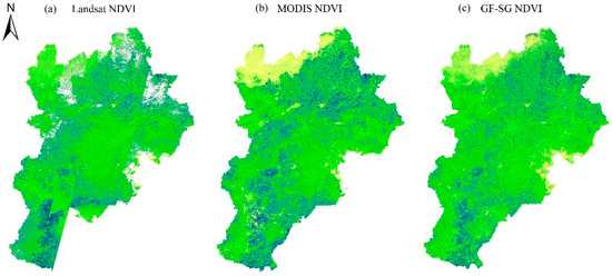
Figure 2.
NDVI fusion results: a general overview.
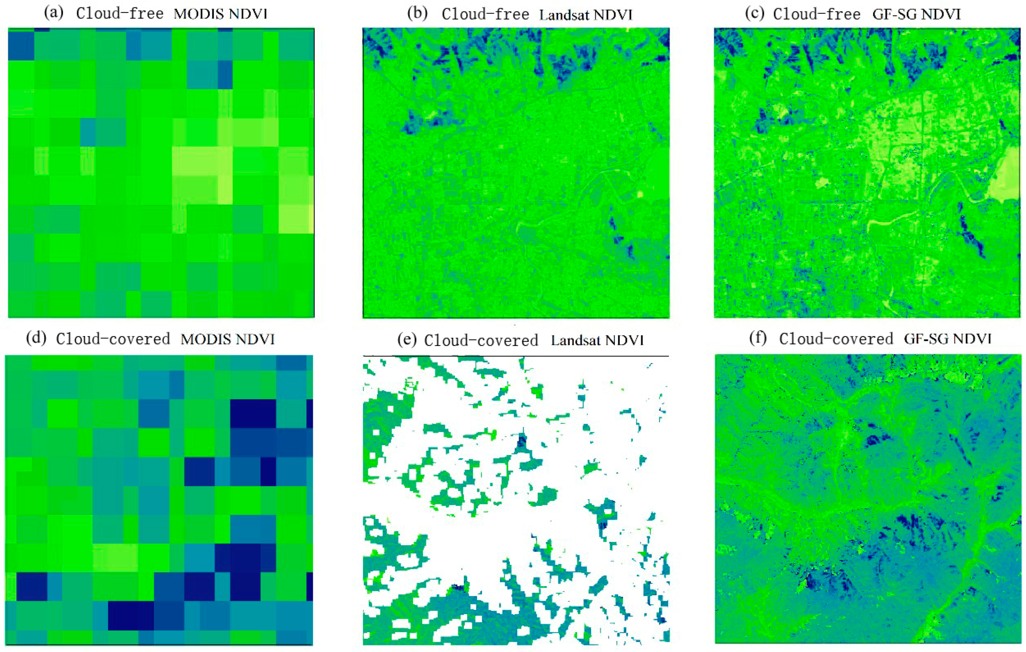
Similarly, taking January 2020 as an example, two 10 km × 10 km areas were randomly selected from both cloud-covered and cloud-free zones within that month’s Landsat images. Figure 3 provides a local view of the NDVI data before and after the fusion process. Compared to the MODIS NDVI data, the spatial resolution of the fused data has been significantly improved. Additionally, the NDVI data for cloud-covered areas before and after fusion show that the GF-SG NDVI successfully filled in the gaps in Landsat NDVI, maintaining consistency with the spatial detail variations in MODIS data.
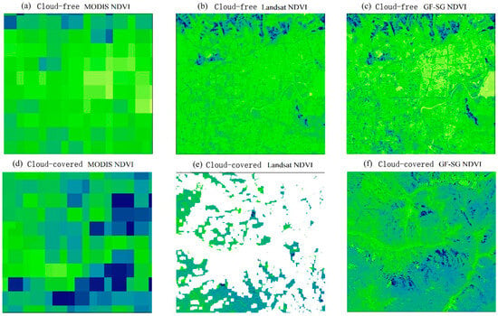
Figure 3.
NDVI fusion results: local view. (a–c) are MODIS, Landsat, and GF-SG NDVI in cloud-free zones; (d–f) are MODIS, Landsat, and GF-SG NDVI in cloud-covered zones.
For the validation of the fused NDVI data, we again used the monthly maximum NDVI values for January 2020 as an example. The validation areas were categorized into cloud-covered, cloud-free, and Landsat image missing zones, and a 10 × 10 km area was randomly selected from each validation zone to validate the fused NDVI data. Given that Sentinel-2 NDVI data have higher spatial and temporal resolution than both Landsat NDVI and MODIS NDVI, Sentinel-2 NDVI data were used as the actual NDVI values to validate the accuracy of the fused GF-SG NDVI data. The validation results are shown in Table 3.

Table 3.
Accuracy evaluation of GF-SG NDVI fusion results.
According to Table 3, the RMSE for the fused GF-SG NDVI data in all three validation zones is below 0.15, indicating a good level of accuracy. The MAE values are all below 0.1, also falling within acceptable limits. The correlation coefficients between the fused NDVI and reference images are all above 0.6, with P values passing the significance test at the 0.05 level, indicating a strong correlation between the fused NDVI and the reference images. Additionally, all three metrics for the fused data outperform those of the MODIS images across all validation zones. The RMSE and MAE values for Landsat NDVI data in cloud-free zones are worse compared to the fused data, with only slight differences in the R values, which demonstrates that the GF-SG NDVI significantly improves the quality of NDVI data, making it closer to actual NDVI values compared to MODIS data. The three metrics indicate that the fused NDVI has a high correlation with the reference images and low error, making it suitable for subsequent NPP and NEP estimation.
3.2. Spatiotemporal Analysis of Carbon Sink Changes
3.2.1. NPP/NEP Estimation and Validation
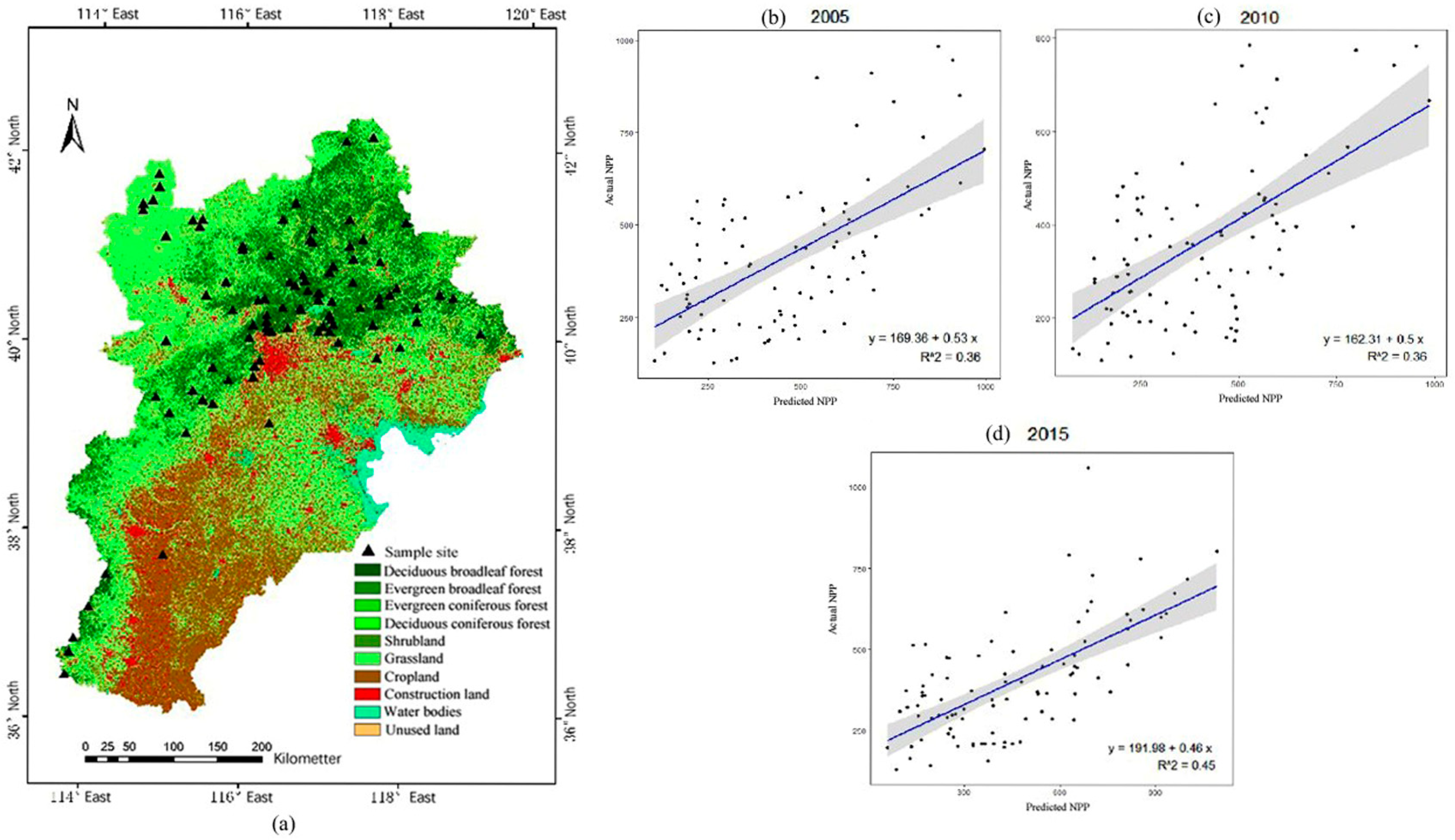
Based on the fused GF-SG NDVI data, this study estimated the NPP and NEP for the study area using the CASA model (see Section 2.3.2) and validated the results. Figure 4 shows the spatial distribution of 92 sample points and the scatter plot of actual NPP versus simulated NPP for three time periods. The shaded gray area in the scatter plot represents the 95% confidence interval.

Figure 4.
Sample points. (a) Spatial distribution of sample points in the BTH region. (b–d) are scatter plots of actual vs. simulated NPP in 2005, 2010, and 2015.
Table 4 displays the Pearson correlation coefficients, MAPE, and RMSE between the measured NPP and the estimated NPP in this study. The correlation coefficients between the estimated and actual NPP values are all above 0.6, with P values reaching the 0.05 significance level, indicating a strong correlation between the predicted and actual values. In this study, the RMSE values for all three years are under 200 gC/m²·a, which is acceptable within the scale of NPP values. A MAPE approaching 0.0 indicates excellent predictions; values below 0.5 are considered acceptable, while values above 0.5 suggest inaccurate predictions [42]. In this study, the MAPE is below 50%, suggesting that the prediction results are acceptable.

Table 4.
Correlation coefficients, MAPE, and RMSE between actual and estimated NPP.
NEP values were calculated based on NPP using the equation from Section 2.3.2. Since vegetation NEP in a region is often used to analyze the carbon sink of that region, NEP is used as a proxy for the carbon sink in this study for the spatiotemporal analysis.
3.2.2. Temporal Analysis of NEP
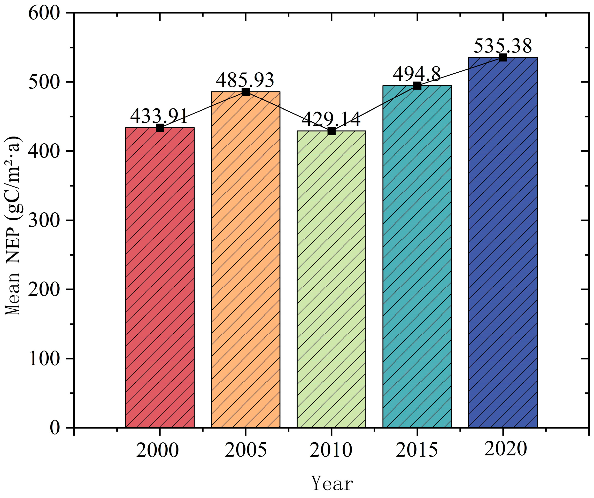
Based on the estimated NEP values for the BTH region from 2000 to 2020, further time series analysis was conducted using the Sen+MK trend analysis method (Figure 5). The results indicate that the BTH region as a whole acts as a carbon sink. The carbon sink capacity of the region showed an increasing trend from 2000 to 2005, a decreasing trend from 2005 to 2010, followed by a gradual increase from 2010 to 2020. Between 2000 and 2020, the region’s carbon sink capacity reached its lowest point in 2010 at 429.14 gC/m²·a and peaked in 2020.
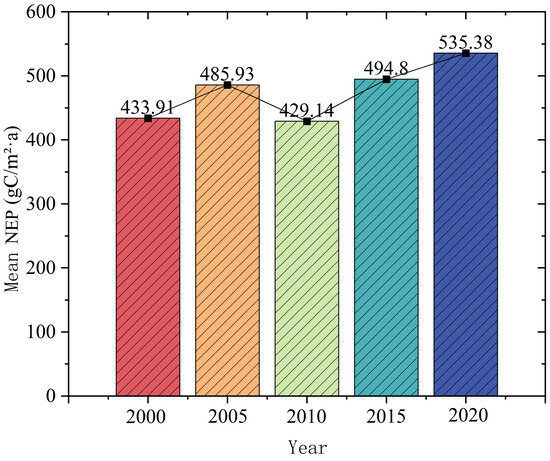
Figure 5.
Time series of mean NEP in the BTH region from 2000 to 2020.
3.2.3. Spatial Analysis of NEP Distribution Changes
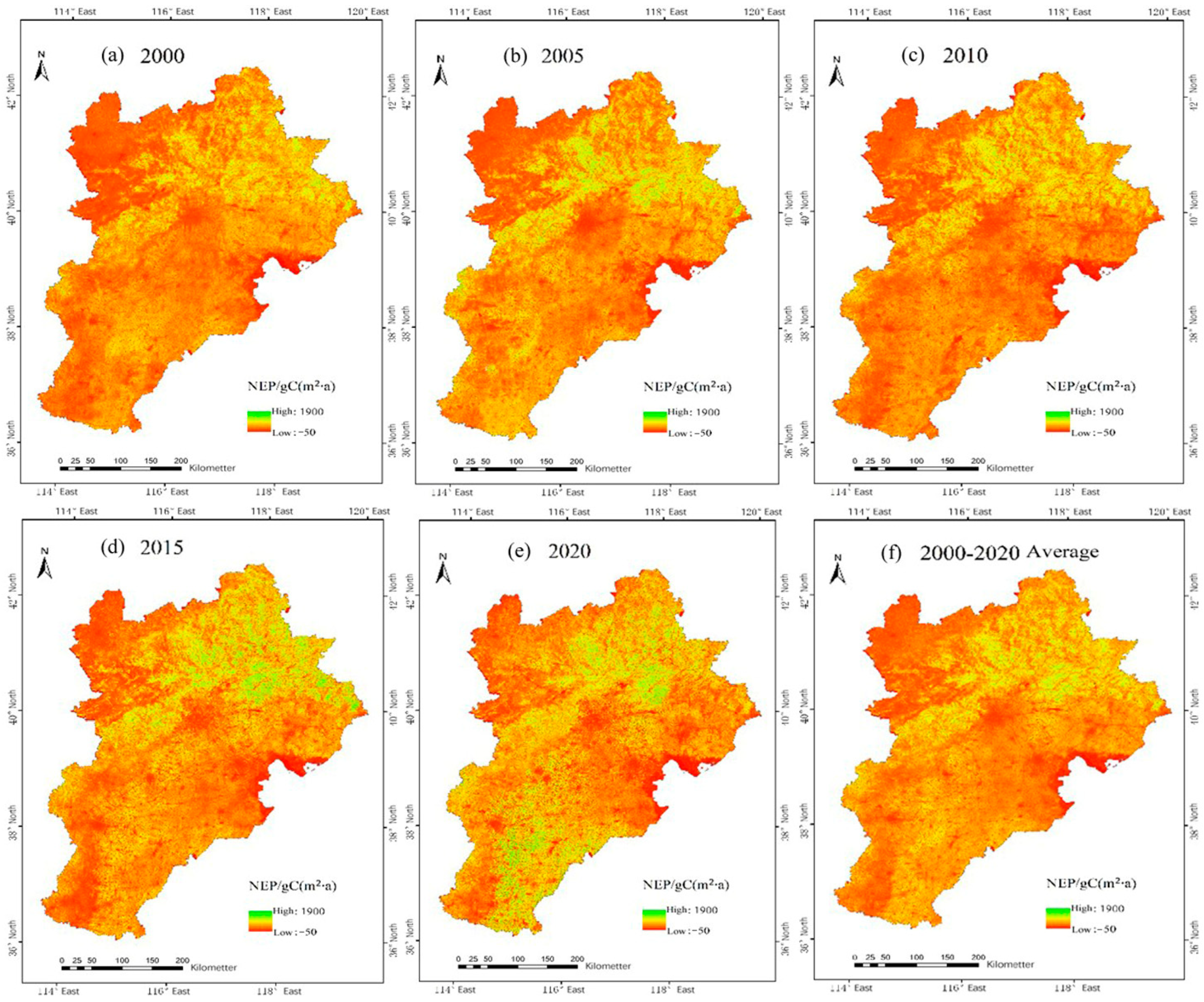
Analyzing the spatial distribution of NEP over five-year intervals from 2000 to 2020 (Figure 6), it can be observed that the NEP shows a pattern of low values in the northwest, central urban areas of Beijing and Tianjin, and coastal regions, moderate values in the North China Plain, and high values in the northern Yanshan–Taihang Mountains. Therefore, the weak carbon sink regions in the BTH area are located in the northwest Bashang Plateau, central urban areas, and coastal regions, which is likely related to the low vegetation coverage in these areas. The North China Plain is classified as a moderate carbon sink region primarily because it is composed of croplands. NEP is high during the crop-growing season but decreases during the colder months when crops are not suitable for growth, leading to this classification. The northern Yanshan–Taihang Mountains region, on the other hand, is a strong carbon sink region, mainly due to its high forest coverage. According to forest inventory data, the major tree species in this area include oak, cypress, poplar, pine, elm, linden, and larch.
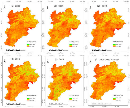
Figure 6.
Spatial distribution of NEP in the BTH region from 2000 to 2020.
In addition, the carbon sink capacity of the Bashang Plateau has continuously improved from 2000 to 2020. The North China Plain has seen a clear overall increase in carbon sink capacity, although it experienced a decline from 2010 to 2015. The central urban areas of Beijing and Tianjin have also shown an overall upward trend in carbon sink capacity, with a decline from 2000 to 2010, followed by an increase from 2010 to 2020. It is worth noting that the Xiong’an New Area, established in 2017 as an important part of the Beijing–Tianjin–Hebei (BTH) coordinated development strategy, is located in the central Hebei province between Beijing, Tianjin, and Baoding. The development of this region has attracted significant attention in recent years. According to Figure 6, from 2015 to 2020, the NEP of Xiong’an New Area showed a stable improvement, and its carbon sink capacity should continue to be protected during future development.
A statistical analysis of the average NEP changes for each city in the BTH region from 2000 to 2020 (Table 5) shows that, overall, all cities except for Tianjin and Qinhuangdao experienced an initial increase in NEP from 2000 to 2005, followed by a decrease from 2005 to 2010, and a continuous increase from 2010 onwards. Cities in the northwest and southern parts of the BTH region, including Zhangjiakou, Chengde, Beijing, Baoding, Langfang, Shijiazhuang, Cangzhou, Xingtai, Hengshui, and Handan, all show increasing trends in NEP. Among these cities, Xingtai experienced the largest increase in NEP, with an increase of 249.82 gC/m²·a over 20 years, while Langfang had a relatively modest increase, with a rise of only 27.67 gC/m²·a.

Table 5.
Mean annual NEP of each city from 2000 to 2020 (unit: gC/m²·a).
In contrast, the cities of Qinhuangdao, Tangshan, and Tianjin, located in the northeastern part of the BTH region, experienced a decline in NEP, with decreases of 186.57 gC/m²·a, 62.83 gC/m²·a, and 16.93 gC/m²·a, respectively. The industrial structures of these cities include a significant presence of environmentally damaging industries such as cement, building materials, steel, glass, fertilizers, and coal, which contribute to environmental pollution. These cities should adjust their industrial structures, reduce the proportion of these industries, or implement and strengthen pollution control measures.
Using the Sen+MK trend analysis method, the NEP for the BTH region from 2000 to 2020 was analyzed (Figure 7). The NEP showed an overall increasing trend, as seen in the trend variation pie chart. About three-fifths of the region showed an upward trend, with areas of strong significant increase accounting for 3.2% of the total area, mainly located in the southern part of the Bashang Plateau. About two-fifths of the region showed a downward trend, with 3.5% of the area experiencing a strong significant decrease, mainly in the northern part of the Bashang Plateau. The ecological conservation areas in Chengde, Zhangjiakou, and the northwestern part of Beijing showed clear improvements in NEP, likely due to long-term forest protection programs such as the Three-North Shelterbelt Project and other ecological policies. Meanwhile, Tianjin, Qinhuangdao, and Tangshan experienced significant declines in NEP, which are related to their industrial structures and land cover types. Other cities showed both improvement and decline in NEP trends, but areas of improvement were generally larger.
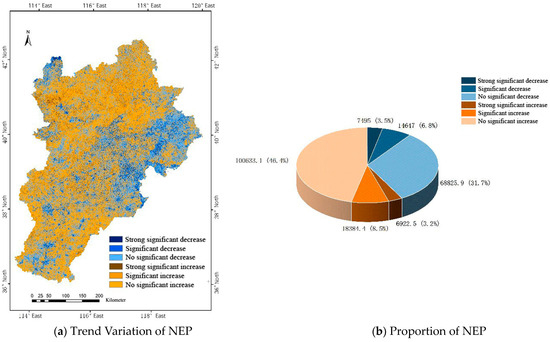
Figure 7.
NEP for the BTH region from 2000 to 2020.
3.3. Response of Carbon Sinks to Land Use Intensity
3.3.1. Bivariate Spatial Autocorrelation Analysis of NEP and Land Use Intensity
Using Moran’s bivariate spatial autocorrelation statistics, the Moran’s I values for land use intensity and NEP in 2000, 2010, and 2020 (Table 6) were all negative, indicating a negative correlation between the two variables. To further verify the credibility of the results, the P values and Z scores were examined. After 999 random permutations of the Moran’s I results, the P values were all less than or equal to 0.01, and the absolute values of the Z scores were greater than 2.58, confirming that the calculated Moran’s I indices were statistically significant. This indicates a significant spatial negative correlation between land use intensity and NEP.

Table 6.
Moran’s bivariate global spatial correlation indices for LUI and NEP from 2000 to 2020.
The bivariate Moran’s I values for land use intensity and NEP were relatively low in 2000 and 2020 but higher in 2000 than in 2020. In 2010, the values increased significantly compared to 2000 and 2020, indicating that the influence of land use intensity on NEP was highest in 2010, followed by 2000 and then 2020. The impact of land use intensity on NEP increased notably in 2010, exceeding 0.3. This suggests that the decline in NEP observed earlier could be linked to the strengthening influence of land use intensity on NEP.
3.3.2. Bivariate Spatial Clustering Analysis of Land Use Intensity and NEP
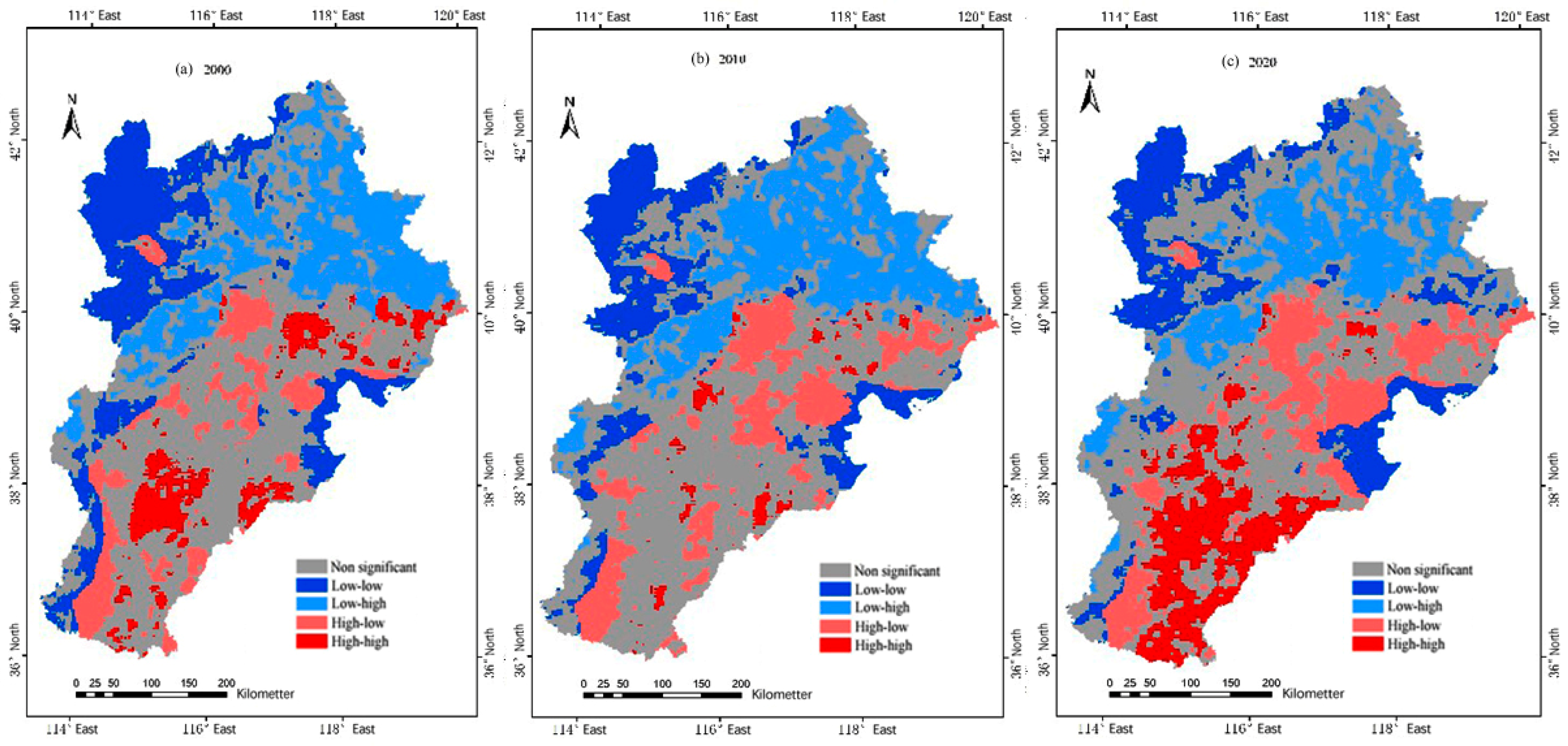
Based on the bivariate LISA clustering maps of NEP and land use intensity from 2000 to 2020 (Figure 8), the low-high clustering areas for land use intensity and NEP were primarily located in the eastern parts of Chengde and Zhangjiakou in northeastern BTH. These areas had relatively low land use intensity but relatively high NEP, indicating a negative spatial correlation between NEP and land use intensity. In 2000, these low-high clustering areas were relatively scattered, became more concentrated in 2010, and decreased again in 2020.

Figure 8.
LISA clustering of NEP and LUI in the BTH region from 2000 to 2020.

Table 7.
Area occupied by the correlation of LUI on NEP in the BTH region from 2000 to 2020 (unit: km2).
Low-low clustering areas indicate regions with low land use intensity and relatively low NEP. These areas are primarily distributed in the northwestern Bashang Plateau, characterized by high altitudes, sparse forests, and low land use intensity. From 2000 to 2020, the low-low clustering areas in the northwest gradually diminished, transitioning into non-significant regions. Additionally, low-low clustering areas were observed in the nearshore and coastal regions of Bohai Bay. These areas are mostly comprised of seawater, rocky coasts, gravel beaches, and muddy shores, contributing to low NEP and low land use intensity. By 2020, the low-low clustering areas in Bohai Bay extended inland towards Cangzhou.
High-low clustering areas, characterized by high land use intensity and low NEP, are mainly found in the central urban areas of Beijing and Tianjin, the middle areas between Handan and Xingtai in the south, and parts of Zhangjiakou. These regions are mostly urban areas or croplands, which carry high land use intensity weights, leading to a negative spatial correlation between land use intensity and NEP. From 2000 to 2010, the high-low clustering areas expanded, indicating an increase in regions where land use intensity negatively impacted NEP. However, these areas slightly decreased between 2010 and 2020.
High-high clustering areas, where both land use intensity and NEP are high, are primarily located in the southeastern regions and cities such as Qinhuangdao, Tangshan, Tianjin, and Langfang. In 2010, many of these high-high clustering areas transitioned into high-low clustering or non-significant regions, indicating an increased negative spatial correlation between land use intensity and NEP. By 2020, parts of these regions turned into low-low clustering areas, suggesting a decrease in land use intensity. Overall, high-high clustering areas were mainly concentrated in the southeastern part of the study region in both 2000 and 2020, though they significantly decreased in 2010, leaving only a few scattered areas in the eastern part of the region.
Non-significant regions were distributed throughout the BTH region, with relatively more non-significant areas in the southeastern part and fewer in the northwest during 2000 and 2010. This indicates that from 2000 to 2010, land use intensity had a greater impact on NEP in the northwest than in the southeast. By 2020, the non-significant regions decreased, and areas with significant correlations increased, indicating that by 2020, more areas were influenced by land use intensity, especially in the southeast, where the positive spatial correlation between land use intensity and NEP had greatly increased.
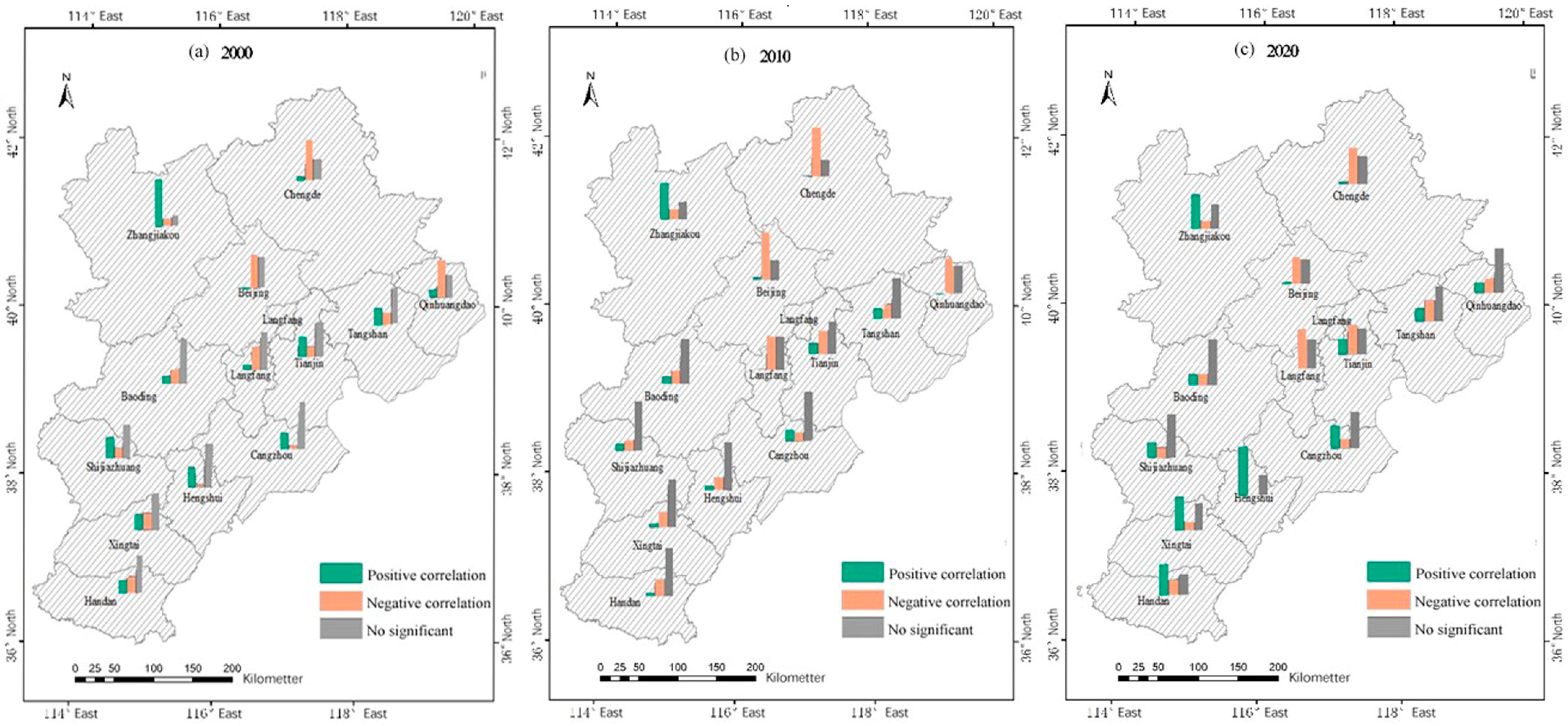
The spatial correlation between land use intensity and NEP at the city level was statistically analyzed, and the results are shown in Figure 9.
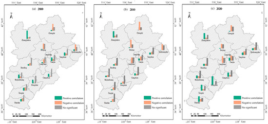
Figure 9.
Spatial correlation between LUI and NEP in each city in the BTH region (2000–2020).
According to Figure 9, in 2000 and 2010, the southeastern cities of Tangshan, Tianjin, Langfang, Cangzhou, Baoding, Shijiazhuang, Hengshui, Xingtai, and Handan were mostly non-significant areas, indicating that land use intensity had no significant impact on NEP in these regions. However, by 2020, Langfang and Tianjin had the most negative spatial correlation areas, indicating that the impact of land use intensity on NEP had shifted from non-significant to negative. Meanwhile, Hengshui, Xingtai, and Handan had the most positive spatial correlation areas, meaning that the effect of land use intensity on NEP had shifted from non-significant to positive. In Qinhuangdao, the areas with the most negative correlations in 2000 and 2010 became non-significant areas by 2020, suggesting that the impact of land use intensity on NEP changed from negative to non-significant. Zhangjiakou consistently had the most positive correlation areas, while Chengde and Beijing were consistently dominated by negative correlation areas.
4. Discussion
In this study, the GF-SG method was used to fuse Landsat and MODIS NDVI data, reconstructing NDVI data with a resolution of 30 m and an 8-day temporal scale. The reconstructed GF-SG NDVI showed significant improvement in quality across all three validation zones—cloud-covered, cloud-free, and Landsat-missing areas. This finding aligns with the results of Chen et al. [12], further validating the effectiveness of the GF-SG method for image fusion and reconstruction. The reconstructed GF-SG NDVI provided high-precision image data for the estimation of NPP and NEP. Using the CASA model, we estimated NPP and NEP in the study area with a spatial resolution of 30 m, and the results showed a strong correlation with actual NPP values, meeting the practical needs of the study. This study further advances the analysis of carbon sinks using remote sensing techniques. Jose et al. (2017) demonstrated the importance of high-resolution data in biomass mapping by applying Sentinel imagery to estimate above-ground biomass in Philippine mangroves [43]. Similarly, our research highlights the critical role of high-resolution data in enhancing carbon sink assessments. Additionally, it provides a more refined data foundation for future studies on the spatial heterogeneity of carbon sinks and their underlying response mechanisms.
This study builds upon international advancements in remote sensing-based carbon sink analysis. Our research underscores the value of finer NDVI resolutions in advancing carbon sink assessments. The implications extend to policy and practice, particularly in enhancing land management strategies to mitigate negative human impacts on carbon sinks.
With the improvement in data quality, the carbon sink estimates in this study were higher than those from studies by Liu (1 km resolution) [44] and Wang et al. (1 km resolution) [9] using the CASA model. When compared with estimates from other carbon sink models, the results varied. The average carbon sink estimate in this study was higher than that derived from the BIOME-BGC model’s MOD17A3 product [45], consistent with the conclusion of Li et al. [46], which stated that carbon sink values estimated using the CASA model at a 30m resolution tend to be higher than those from the BIOME-BGC model at a 1 km resolution. However, when compared with the Resdc NPP estimates using the GLO_PEM model at 1 km resolution, this study’s estimates for carbon sinks in coniferous forests and grasslands were higher, while those for the other three vegetation types were lower.
Spatially, the carbon sink estimates in the BTH region classified weak carbon sink areas as the northwest Bashang Plateau, central urban areas, and coastal regions; strong carbon sink areas as the northern Yanshan–Taihang Mountains; and moderate carbon sink areas as the North China Plain cropland regions. These findings are highly consistent with those of Wang et al. (1 km resolution) [9] in terms of weak and strong carbon sink distributions. However, the spatial trend results differ; from 2000 to 2020, this study observed an overall improving trend in carbon sink capacity, whereas Wang’s study indicated a decreasing trend in the central and coastal regions of the BTH area.
This study used land use intensity indicators to quantitatively evaluate the dynamic changes in the impact of human activities on carbon sinks in the BTH region. A significant spatial negative correlation was observed between land use intensity and carbon sink values, indicating that increased human activity generally reduces carbon sink capacity. This is consistent with Zhang’s conclusions [47]. The expansion of construction land directly reduces vegetation coverage, thereby diminishing carbon sink capacity. Additionally, high cropping intensity often results in soil degradation, reduced organic matter, and nutrient loss, which negatively impact NPP and NEP. Spatially, land use intensity in the BTH region showed a distribution pattern of low intensity in the northwest, high intensity in the southeast and central urban areas, and a transition zone in the central east, which is related to the high proportion of construction land. Due to the significant impact of human activities on construction land and cropland, these land types carried higher weights in the calculation of land use intensity. As a result, the spatial distribution of land use intensity differs from the spatial distribution of land use itself.
While this study made some advances in the accuracy of carbon sink estimation and response mechanism analysis, there are still limitations. First, although the GF-SG method performed well in reconstructing NDVI, further research and optimization of spatiotemporal data fusion methods are needed to obtain higher precision NDVI data, which would further improve the accuracy of NPP and NEP estimates. Second, in terms of carbon sink response mechanisms, this study only considered the impact of land use. In future studies, the influence of socioeconomic factors, such as GDP, population, and road network density, on NPP and NEP should also be included to provide a more comprehensive analysis of the driving mechanisms of NPP and NEP from a socioeconomic perspective. Third, one limitation of NDVI is its saturation effect when chlorophyll content and the LAI value of the vegetation canopy increase. In this study, we partially mitigated the saturation issue in high-brightness regions by fusing MODIS and NDVI data, leveraging the complementary strengths of both datasets. However, due to constraints in data availability and technological capabilities, the saturation problem could not be fully resolved. Future research should aim to address this issue more comprehensively by optimizing both data sources and analytical methods.
5. Conclusions
This study fused Landsat and MODIS NDVI data using the GF-SG method, then estimated NEP in the BTH region using the CASA model. The spatiotemporal changes in NEP were analyzed using the Sen+MK trend analysis method. Furthermore, bivariate spatial autocorrelation analysis and bivariate LISA clustering were used to explore the response of NEP to land use intensity. The main conclusions are as follows:
(1) The fused GF-SG NDVI data provided high-precision image data for the estimation of NPP and NEP. By further applying the CASA model, high-resolution NPP and NEP data with a spatial resolution of 30 m were obtained for the study area;
(2) From 2000 to 2020, the overall trend in the BTH region showed an improvement in carbon sink capacity. The weak carbon sink areas were the northwest Bashang Plateau, central urban areas, and coastal regions, while the strong carbon sink areas were in the northern Yanshan–Taihang Mountains, and the moderate carbon sink areas were the cropland regions of the North China Plain;
(3) There was a significant overall spatial negative correlation between land use intensity and NPP/NEP in the BTH region. Land use intensity followed a pattern of low intensity in the northwest, high intensity in the southeast and central areas, and a transitional zone in the central east.
Author Contributions
Conceptualization, L.C.; methodology, Q.Y. and J.Z.; formal analysis, H.S., R.Y., N.X. and J.W.; investigation, H.S., R.Y., N.X. and J.W.; writing—original draft preparation, Q.Y. and J.Z.; writing—review and editing, Q.Y., J.Z., H.S., R.Y., N.X., J.W. and L.C.; visualization, Q.Y., J.Z., H.S., R.Y., N.X., J.W. and L.C.; supervision, L.C.; funding acquisition, J.W. All authors have read and agreed to the published version of the manuscript.
Funding
This research was funded by the Fundamental Research Funds for the Natural Science Foundation of China (grant number 42330507) and the Beijing Natural Science Foundation Program (grant numbers 8212031 and 8222052).
Data Availability Statement
Data is contained within the article.
Acknowledgments
We are grateful to the teachers at Beijing Forestry University and the staff of Beijing Municipal Institute of City Management.
Conflicts of Interest
The authors declare no conflicts of interest.
References
- Fang, J.; Chen, A. Dynamic changes and significance of China’s forest vegetation carbon pool. Chin. Bull. Bot. 2001, 43, 967–973. [Google Scholar] [CrossRef]
- Wu, Q.; Yao, X.; Liang, J.; Zhang, S.; Yang, Y.; Hou, H. Temporal and spatial intensity of vegetation cover improvement and degradation effects in coal mining areas of Ordos City. J. Arid Land Resour. Environ. 2022, 36, 101–109. [Google Scholar] [CrossRef]
- Qin, L.; Chen, B.; Yu, Y.; Yang, J.; Yang, Y. Study on the spatial and temporal variation of ecological environment before and after mine closure based on remote sensing ecological index. Met. Mine 2023, 3, 242–249. [Google Scholar] [CrossRef]
- Shukla, P.R.; Skeg, J.; Calvo Buendia, E.; Masson-Delmotte, V.; Pörtner, H.-O.; Roberts, D.C.; Zhai, P.; Slade, R.; Connors, S.; van Diemen, S.; et al. Climate Change and Land: An IPCC Special Report on Climate Change, Desertification, Land Degradation, Sustainable Land Management, Food Security, and Greenhouse Gas Fluxes in Terrestrial Ecosystems; Intergovernmental Panel on Climate Change: Geneva, Switzerland, 2019. [Google Scholar]
- Wang, S.; Zhang, Y.; Ju, W.; Chen, J.M.; Ciais, P.; Cescatti, A.; Sardans, J.; Janssens, I.A.; Wu, M.; Berry, J.A.; et al. Recent global decline of CO2 fertilization effects on vegetation photosynthesis. Science 2020, 370, 1295–1300. [Google Scholar] [CrossRef]
- Bader, Y.; Ganguli, S. Analysis of the association between economic growth, environmental quality and health standards in the Gulf Cooperation Council during 1980-2012. Manag. Environ. Qual. Int. J. 2019, 30, 1050–1071. [Google Scholar] [CrossRef]
- Wang, D.; Cao, Z.; Zhang, L.; Chen, J.; Qu, M.; Xin, Y.; Fan, H. Study on the spatial and temporal distribution of NPP and its influencing factors in the Beijing-Tianjin-Hebei urban agglomeration. Environ. Ecol. 2020, 2, 1–10. [Google Scholar]
- Gao, X.; Yu, C.; Zhang, J.; Zhang, J. Quantitative evaluation of the relative effects of climate change and human activities on Net Primary Productivity in Beijing-Tianjin-Hebei. Chin. J. Agrometeorol. 2022, 43, 124–136. [Google Scholar] [CrossRef]
- Wang, J.; Zhao, A.; Zhang, Z. Temporal and spatial evolution and driving factors of vegetation net primary productivity in the Beijing-Tianjin-Hebei region from 2000 to 2018. Chin. J. Ecol. Sci. 2021, 40, 103–111. [Google Scholar] [CrossRef]
- Chen, Y.; Cao, R.Y.; Chen, J.; Zhu, X.L.; Zhou, J.; Wang, G.P.; Shen, M.G.; Chen, X.H.; Yang, W. A new cross-fusion method to automatically determine the optimal input image pairs for NDVI spatiotemporal data fusion. IEEE Trans. Geosci. Remote Sens. 2020, 58, 5179–5194. [Google Scholar] [CrossRef]
- Moreno-Martínez, A.; Izquierdo-Verdiguier, E.; Maneta, M.P.; Camps-Valls, G.; Robinson, N.; Muñoz-Marí, J.; Sedano, F.; Clinton, N.; Running, S.W. Multispectral high resolution sensor fusion for smoothing and gap-filling in the cloud. Remote Sens. Environ. 2020, 247, 111901. [Google Scholar] [CrossRef]
- Chen, Y.; Cao, R.; Chen, J.; Liu, L.; Matsushita, B. A practical approach to reconstruct high-quality Landsat NDVI time-series data by gap filling and the Savitzky–Golay filter. ISPRS J. Photogramm. Remote Sens. 2021, 180, 174–190. [Google Scholar] [CrossRef]
- Potter, C.S.; Randerson, J.T.; Field, C.B.; Matson, P.A.; Vitousek, P.M.; Mooney, H.A.; Klooster, S.A. Vulnerability of permafrost carbon to climate change: Implications for the global carbon cycle. BioScience 2008, 58, 701–714. [Google Scholar] [CrossRef]
- Potter, C.S.; Randerson, J.T.; Field, C.B.; Matson, P.A.; Vitousek, P.M.; Mooney, H.A.; Klooster, S.A. Terrestrial ecosystem production: A process model based on global satellite and surface data. Glob. Biogeochem. Cycles 1993, 7, 811–841. [Google Scholar] [CrossRef]
- Field, C.B.; Behrenfeld, M.J.; Randerson, J.T.; Falkowski, P. Primary production of the biosphere: Integrating terrestrial and oceanic components. Science 1998, 281, 237–240. [Google Scholar] [CrossRef] [PubMed]
- Gao, Q.; Wan, Y.; Li, Y.; Sheng, W.; Jiangcun, W.; Wang, B.; Li, F. Trends in NPP in the alpine grasslands of Northern Tibet and their response to human activities. Acta Ecol. Sin. 2007, 27, 4612–4619. [Google Scholar] [CrossRef]
- Sun, H.; Zheng, D.; Yao, T.; Zhang, Y. National ecological security barrier protection and construction on the Qinghai-Tibet Plateau. Acta Geogr. Sin. 2012, 67, 3–12. [Google Scholar]
- Liu, J. Simulation and Prediction of Net Primary Productivity in Forest Ecosystems in the Qinling Mountains. Master’s Thesis, Northwest University, Kirkland, WA, USA, 2019. [Google Scholar]
- Zhu, W.; Pan, Y.; Zhang, J. Remote sensing estimation of net primary productivity of terrestrial vegetation in China. Chin. J. Plant Ecol. 2007, 31, 413–424. [Google Scholar]
- Liu, Z.; Hu, M.; Hu, Y.; Wang, G. Estimation of net primary productivity of forests by modified CASA models and remotely sensed data. Int. J. Remote Sens. 2017, 39, 1092–1116. [Google Scholar] [CrossRef]
- Qiu, S.; Liang, L.; Wang, Q.; Geng, D.; Wu, J.; Wang, S.; Chen, B. Estimation of European Terrestrial Ecosystem NEP Based on an Improved CASA Model. IEEE J. Sel. Top. Appl. Earth Obs. Remote Sens. 2023, 16, 1244–1255. [Google Scholar] [CrossRef]
- Chen, Y.; Luo, G.; Maisupova, B.; Chen, X.; Mukanov, B.M.; Wu, M.; Mambetov, B.T.; Huang, J.; Li, C. Carbon budget from forest land use and management in Central Asia during 1961–2010. Agric. For. Meteorol. 2016, 221, 131–141. [Google Scholar] [CrossRef]
- Yang, Y.; Song, G. Human disturbance changes based on spatiotemporal heterogeneity of regional ecological vulnerability: A case study of Qiqihar city, northwestern Songnen Plain, China. J. Clean. Prod. 2021, 291, 125262. [Google Scholar] [CrossRef]
- Feng, X.; Li, Y.; Yu, E.; Yang, J.; Wang, S.; Ma, J. Spatiotemporal pattern and coordinated development characteristics of carbon emission performance and land use intensity in the Yangtze River Delta urban agglomeration. Trans. Chin. Soc. Agric. Eng. 2023, 39, 208–218. [Google Scholar] [CrossRef]
- Wang, X. Study on the Spatiotemporal Evolution of Human Activity Disturbance Intensity and Habitat Quality at the County Level Based on Spatial Quantification Model. Master’s Thesis, Beijing University of Civil Engineering and Architecture, Beijing, China, 2023. [Google Scholar]
- Song, W.; Wang, C.; Chen, W.; Zhang, X.; Li, H.; Li, J. Unlocking the spatial heterogeneous relationship between Per Capita GDP and nearby air quality using bivariate local indicator of spatial association. Resour. Conserv. Recycl. 2020, 160, 104880. [Google Scholar] [CrossRef]
- Sakamoto, T.; Wardlow, B.D.; Gitelson, A.A.; Verma, S.B.; Suyker, A.E.; Arkebauer, T.J. A two-step filtering approach for detecting maize and soybean phenology with time-series MODIS data. Remote Sens. Environ. 2010, 114, 2146–2159. [Google Scholar] [CrossRef]
- Qiu, Z. Study on Carbon Sequestration Measurement Methods and Applications in China’s Forest Vegetation. Ph.D. Thesis, Beijing Forestry University, Beijing, China, 2019. [Google Scholar] [CrossRef]
- Liang, B.; Wang, J.; Zhang, Z.; Zhang, J.; Zhang, J.; Cressey, E.L.; Wang, Z. Planted forest is catching up with natural forest in China in terms of carbon density and carbon storage. Fundam. Res. 2022, 2, 688–696. [Google Scholar] [CrossRef] [PubMed]
- Liu, S.; Ruan, H. Spatial pattern analysis of forest biomass and NPP in Guangdong and Guangxi provinces based on geostatistics. Chin. J. Ecol. 2013, 32, 2502–2509. [Google Scholar] [CrossRef]
- Wang, B.; Liu, M.; Zhang, B. Study on forest vegetation net primary productivity and its dynamic changes based on forest inventory data. For. Resour. Manag. 2009, 1, 35–43. [Google Scholar] [CrossRef]
- Wei, X.; Yang, J.; Luo, P.; Lin, L.; Lin, K.; Guan, J. Assessment of the variation and influencing factors of vegetation NPP and carbon sink capacity under different natural conditions. Ecol. Indic. 2022, 138, 108834. [Google Scholar] [CrossRef]
- Liu, F.; Zeng, Y. Analysis of the spatio-temporal variation of vegetation carbon source/sink in Qinghai Plateau from 2000–2015. Acta Ecol. Sinica. 2021, 41, 5792–5803. [Google Scholar] [CrossRef]
- Chen, Y.; Wang, J.; Xiong, N.; Sun, L.; Xu, J. Impacts of land use changes on net primary productivity in urban agglomerations under multi-scenarios simulation. Remote Sens. 2022, 14, 1755. [Google Scholar] [CrossRef]
- Li, X.; Luo, Y.; Wu, J. Decoupling relationship between urbanization and carbon sequestration in the Pearl River Delta from 2000 to 2020. Remote Sens. 2022, 14, 526. [Google Scholar] [CrossRef]
- Rong, T.; Long, L.H. Quantitative assessment of NPP changes in the Yellow River source area from 2001 to 2017. IOP Conf. Ser. Earth Environ. Sci. 2021, 687, 012002. [Google Scholar] [CrossRef]
- Nan, L.; Yang, M.; Hao, S. Analysis of temporal and spatial distribution characteristics of precipitation in Chongqing from 1965 to 2014. Yangtze River 2021, 52, 64–69. [Google Scholar] [CrossRef]
- Shi, J.; Shi, P.; Wang, Z.; Wan, Y. Impact of human disturbance on the dynamic evolution of ecological vulnerability: A case study of the Lanxi urban agglomeration. Chin. Environ. Sci. 2023, 43, 1317–1327. [Google Scholar] [CrossRef]
- Feng, Z.; Zhang, J.; Hou, W.; Zhai, L. Analysis of human disturbance degree to the ecological environment based on land cover classification: A case study of Beijing. Chin. J. Ecol. 2017, 36, 508–516. [Google Scholar] [CrossRef]
- Lu, Z.; Lei, G.; Guo, Y.; Ma, Q. Changes in land use intensity and its impact on climate factors at different spatial scales in the Songnen Plain. Acta Ecol. Sin. 2021, 41, 13. [Google Scholar] [CrossRef]
- Zhang, L.; Hou, Q.; Duan, Y.; Liu, W. Spatial correlation between water resources and rural settlements in the Yanhe watershed based on bivariate spatial autocorrelation methods. Land 2023, 12, 1719. [Google Scholar] [CrossRef]
- Zhou, X. Research on Influencing Factors and Prediction Models of Urban Air Quality Based on Spatial Metrology and Deepensemble Algorithms. Master’s Thesis, Hangzhou Dianzi University, Hangzhou, China, 2024. [Google Scholar] [CrossRef]
- Castillo, J.A.A.; Apan, A.A.; Maraseni, T.N.; Salmo, S.G., III. Estimation and mapping of above-ground biomass of mangrove forests and their replacement land uses in the Philippines using Sentinel imagery. ISPRS J. Photogramm. Remote Sens. 2017, 134, 70–85. [Google Scholar] [CrossRef]
- Liu, G. Remote Sensing Estimation of Net Primary Productivity of Forest Vegetation in the Beijing-Tianjin-Hebei Region. Master’s Thesis, Beijing Forestry University, Beijing, China, 2008. [Google Scholar]
- Zhang, L.; Wu, Z.; Chen, J.; Liu, D.; Chen, P. Spatiotemporal patterns and drivers of net primary production in the terrestrial ecosystem of the Dajiuhu Basin, China, between 1990 and 2018. Ecol. Inform. 2022, 72, 101839. [Google Scholar] [CrossRef]
- Li, C.; Cao, H.; Fan, Y.; Han, H.; Sun, H.; Wang, Y. Remote sensing estimation and analysis of NPP based on a calibrated CASA model: A case study of the Hexi Corridor. Acta Ecol. Sin. 2019, 39, 1616–1626. [Google Scholar] [CrossRef]
- Zhang, J.; Hao, X.; Hao, H.; Fan, X.; Li, Y. Climate change decreased net ecosystem productivity in the arid region of Central Asia. Remote Sens. 2021, 13, 4449. [Google Scholar] [CrossRef]
Disclaimer/Publisher’s Note: The statements, opinions and data contained in all publications are solely those of the individual author(s) and contributor(s) and not of MDPI and/or the editor(s). MDPI and/or the editor(s) disclaim responsibility for any injury to people or property resulting from any ideas, methods, instructions or products referred to in the content. |
© 2024 by the authors. Licensee MDPI, Basel, Switzerland. This article is an open access article distributed under the terms and conditions of the Creative Commons Attribution (CC BY) license (https://creativecommons.org/licenses/by/4.0/).


