Article

Impact of Climate Change on the Potential Geographical Distribution Patterns of Luculia pinceana Hook. f. since the Last Glacial Maximum

1
School of Landscape Architecture and Horticulture Sciences, Southwest Forestry University, Kunming 650224, China
2
Southwest Landscape Architecture Engineering Technology Research Center, State Forestry and Grassland Administration, Kunming 650224, China
3
Key Laboratory of National Forestry and Grassland Administration on Biodiversity Conservation in Southwest China, Kunming 650224, China
*
Author to whom correspondence should be addressed.
Forests 2024, 15(2), 253; https://doi.org/10.3390/f15020253
Submission received: 20 December 2023 / Revised: 21 January 2024 / Accepted: 23 January 2024 / Published: 29 January 2024
(This article belongs to the Section Forest Meteorology and Climate Change)

Abstract

:
In this study, we utilized 76 natural distribution points and six environmental variables to establish a detailed species distribution prediction process for Luculia pinceana Hook. f. Our aim was to explore the potential distribution patterns of L. pinceana since the Last Glacial Maximum (LGM) and its response to climate change, providing a scientific basis for conservation strategies and the suitable introduction of its wild populations. This model enabled the prediction of L. pinceana’s geographical distribution patterns across five temporal phases: the LGM, the Mid-Holocene (MH), the present, and two future scenarios. Additionally, the model pinpointed the dominant environmental factors influencing these distribution patterns. The results indicate the following: (1) The temperature annual range (bio7), the minimum temperature of the coldest month (bio6), and the precipitation of the wettest month (bio13) are the dominant environmental factors that determine the distribution of L. pinceana. In areas where bio7 is less than 22.27 °C, bio6 is above 3.34 °C, and bio13 exceeds 307.65 mm, the suitability for L. pinceana is highest. (2) Under the current climatic conditions, the highly suitable area of L. pinceana accounts for 64 × 104 km2, which accounts for half of the total suitable area. The suitable habitats for L. pinceana are concentrated in Yunnan, Guizhou, Sichuan, Chongqing, Guangxi, southern Nyingchi in Tibet, and the coastal areas of South China. (3) During the LGM and the MH, the suitable habitats for L. pinceana were essentially consistent with the current scenarios, with no significant southward shift in distribution. This lack of a major southward migration during the LGM could be attributed to the species finding refuge in situ in mountainous areas. (4) Under various future emission scenarios, the suitable habitat area for L. pinceana is expected to experience significant expansion, generally shifting towards the northwest and higher latitudes. The anticipated global warming in the future is likely to provide more favorable conditions for the survival of L. pinceana. It is recommended that the introduction follows the direction of centroid migration, facilitated by vegetation management, and it has the ecological and economic benefits of L. pinceana to a greater extent.

1. Introduction

Climate change, a focal topic of the 21st century, has wrought a series of impacts through changes in surface temperature, precipitation, heatwave frequency and intensity, forest fires, and pest outbreaks. These factors collectively alter the adaptability of plants to stress, as well as the structure and function of ecosystems [1,2], and consequently modify the geographic distribution patterns of plants. Such alterations can lead to extensive expansions [3], directly or indirectly causing substantial losses in global biodiversity [4]. The Last Glacial Maximum (LGM, approximately 22,000 years ago) and the Mid-Holocene (MH, about 6000 years ago) represent critical periods for modeling the effects of historical climate changes on plant distribution patterns [5]. According to paleoclimate simulations and palynological data [6,7,8], the global climate during the LGM was drier and colder, with the tropical vegetation in southern China being replaced by subtropical evergreen broadleaf forests. In contrast, the MH period tended towards warm and humid conditions, with temperatures nearing contemporary levels and precipitation initially increasing and then decreasing. This led to a northward shift of 200–500 km in the subtropical evergreen broadleaf and mixed forests of eastern China [5]. Climate plays a pivotal role in the large-scale distribution of species, and the climatic changes from the last glacial period to the present continually influence the global biogeographic distribution of life. Many species that survived the glacial periods have expanded their ranges from refugia following climate warming, forming new geographical distribution patterns [9]. Southwest China, identified as one of the 35 global biodiversity hotspots, is home to numerous ancient and relict species [10]. Past geological and climatic changes have profoundly influenced the genetic patterns and geographic structures of species in this region, making it a key area for global biodiversity. Over recent decades, ongoing global climate change has intensified, with rising temperatures and changing spatial patterns of precipitation [11]. This change is more severe than at any previous time [12], with temperatures expected to rise by 3.0–5.1 °C by the end of the 21st century, affecting various climate variables related to temperature [13,14]. Plants, as crucial components of ecosystems, exert cascading impacts on the environment in terms of resource availability, local climate stability, and ecosystem services when affected. Thus, examining the response of characteristic species in Southwest China to climate change not only facilitates visualization of their geographic distribution patterns and the conservation of biodiversity but also benefits the efficient utilization and management practices of germplasm resources [15].
Luculia pinceana Hook. F., a member of the Rubiaceae family and the Luculia genus, is an evergreen shrub or tree. This plant can reach heights of 2–10 m and is primarily found in the northwest parts of Yunnan and Guangxi provinces in China. It is also distributed in southern Tibet, Guizhou, and Chongqing regions, and extends to Thailand and Vietnam [16]. In recent years, the cultivation of new varieties has emerged as a key focus for the conservation and utilization of L. pinceana. [17,18,19]. Given the ease of artificial cultivation of L. pinceana, it is considered an ideal candidate for the widespread propagation of this genus [20]. L. pinceana mainly grows in forested hillsides or along mountain valley streams, at altitudes ranging from 600 to 3000 m. L. pinceana is highly valued for ornamental purposes, blooming continuously from August to December. Its flowers, clustered in corymbose inflorescences, are high-pedunculate, cup-shaped, and come in shades of white, pink, and purplish-red, exuding a rich fragrance, making it suitable for multi-seasonal landscaping [21]. Additionally, various parts of L. pinceana, including flowers, fruits, and roots, serve as raw materials for medicinal purposes, treating conditions such as bruises, rheumatic pain, menstrual disorders, and hypertension, highlighting its potential as a valuable wild ornamental and medicinal resource [22,23]. Plants living in the Himalayan region show significant reactions to the environmental requirements for precipitation and temperature, especially temperature sensitivity [24]. As a distinctive plant of Southwest China, L. pinceana thrives in warm and humid zones and is sensitive to changes in temperature and rainfall. L. pinceana, influenced by climate and human disturbances, is a rare plant not yet listed in the Red Book [25]. As a thermophilic species, L. pinceana thrives optimally at temperatures of 18–20 °C, with a narrow niche and sensitivity to climate change. Issues regarding its safe overwintering limit its practical applications [26]. Current research on L. pinceana primarily concentrates on areas including variety breeding [17,27], physiological biochemistry [26], pollination mechanisms [28], component analysis [22], and the breeding relevance of its fragrance and nectar [16,29], with limited exploration into the impacts of climate change on its geographic distribution patterns. Considering the increasing severity of contemporary climate change, predicting the trends of spatial geographic distribution patterns of L. pinceana during the last glacial period and under future global warming scenarios, and exploring the main environmental variables limiting its distribution can provide a scientific basis for the introduction, acclimatization, and resource management of L. pinceana’s wild resources in China.
In the theoretical framework of species distribution models (SDMs), the concept of the niche occupies a central position [30]. Hutchinson divided the niche into the fundamental niche and the realized niche [31]. The former encompasses all non-biotic environmental factors necessary for a species’ survival, while the latter extends upon this by considering interspecific interactions [32]. SDMs, assuming a certain equilibrium between species and environmental conditions, utilize species presence or abundance data along with corresponding environmental data to calculate niche requirements, which are then expressed probabilistically. These probabilities are projected onto specific spatiotemporal dimensions to simulate the potential distribution of species in suitable areas during specified periods [30,33,34]. When predicting the suitable areas for species, not only are abiotic and biotic factors taken into account, but species’ migration and adaptation capabilities are also considered influential for the effectiveness of SDMs [35]. The mechanisms of these influencing factors and their contribution rates vary with the scale of study. At smaller scales, interspecies interactions predominantly influence species distribution patterns, with biotic factors contributing more at local scales and topographic factors becoming more significant at the landscape scale, while climatic variables are key in determining habitat suitability at regional and larger scales [35,36]. SDMs have been applied in distribution prediction studies for various taxa, including animals [37], plants [38], insects [39], marine organisms [40], lichens and mosses [41], and viruses [42], often employed in fields like invasive plant risk identification, animal habitat prediction, and pest control, predominantly using single-model approaches, especially MaxEnt [43]. Depending on the algorithm, there are different types of SDMs, and their applicability varies with species and the number of distribution points [44,45], suggesting that no single perfect model algorithm suits all niche characteristics [46]. Therefore, selecting the correct algorithm to minimize uncertainty within the model is a fundamental aspect of prediction work. Biomod2 is a package in R that includes ten commonly used SDMs, allowing users to freely combine and adjust each model’s parameters and environmental factors. Biomod2 surpasses single-algorithm models in both functionality and precision [47].
This study, starting from the distinctive plant L. pinceana in Southwest China, utilizes Biomod2 to combine optimal models for simulating the geographic distribution patterns of L. pinceana across five periods: the LGM, the MH, current (1970–2000), and future (2050s: 2041–2060, and 2090s: 2081–2100). It also calculates the migration trajectories of the suitable area centroids and the contribution of environmental variables, aiming to provide a theoretical basis and reference for the conservation and scientific introduction and cultivation of L. pinceana.

2. Materials and Methods
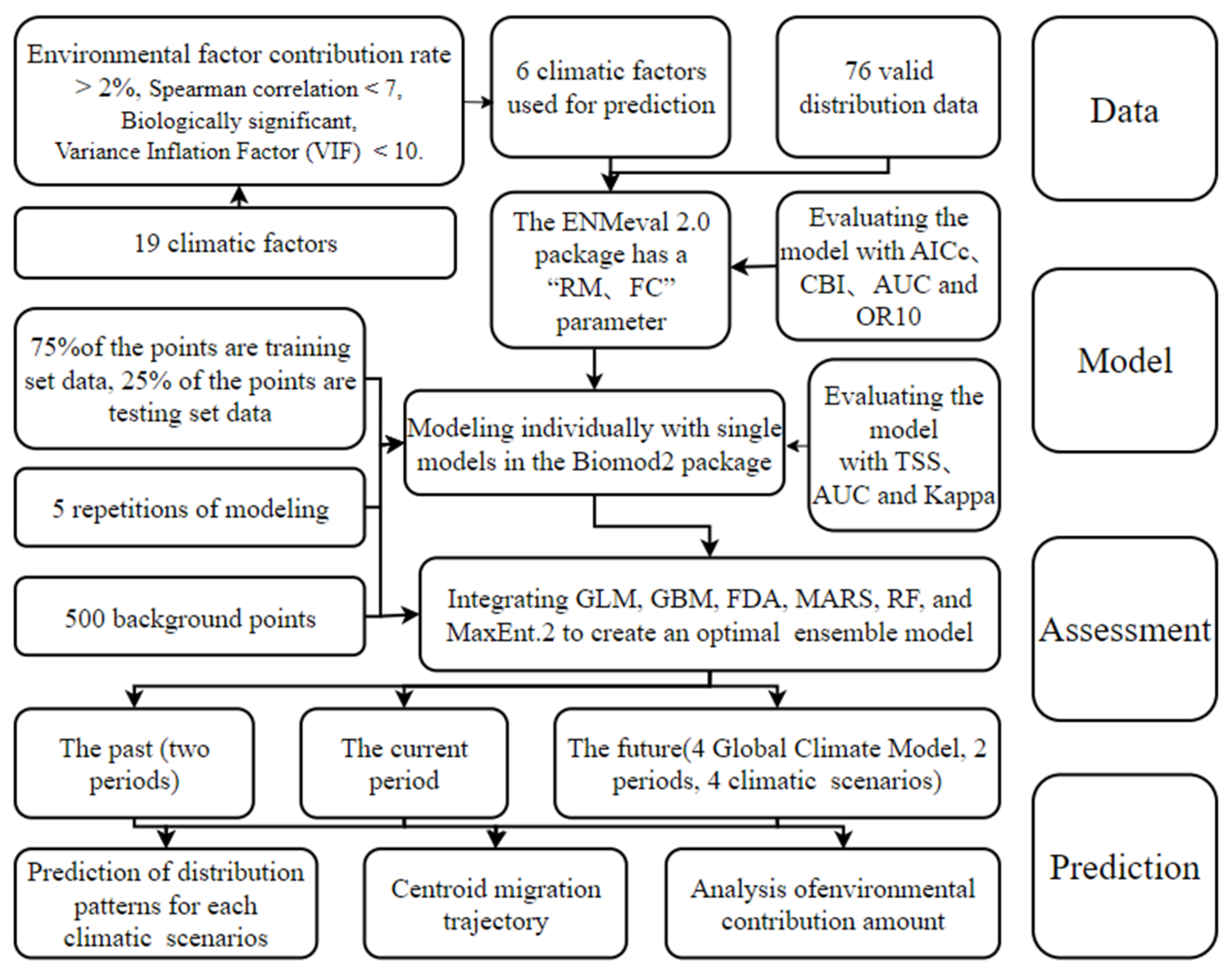
2.1. Workflow

In this study, following the standard protocol for species distribution models (SDMs), we established the ODMAP (Overview, Data, Model, Assessment and Prediction) and the ecological niche simulation workflow diagram [14,48]. The methodology for constructing and analyzing SDMs encompasses five integral components: an Overview of the research context and objectives, Data acquisition and preprocessing, Model development and selection, Assessment of model performance and validity, and Prediction of species distributions. This paper rigorously details the ecological niche simulation workflow (Figure 1) to ensure the research’s transparency, reproducibility, and facilitation of a rigorous peer review and expert appraisal of the model’s robustness and accuracy.

2.2. Collection of Distribution Points

Our data were sourced from relevant literature and databases to gather distribution data of L. pinceana. The sources of our data included the Global Biodiversity Information Facility (GBIF.org GBIF Occurrence Download https://doi.org/10.15468/dl.hh8arv/ (accessed on 15 November 2022)), the National Natural Science Resources Platform Teaching Specimen Resource Sharing Platform Museum (http://mnh.scu.edu.cn/ (accessed on 3 January 2023)), the National Specimen Information Infrastructure (NSII: http://www.nsii.org.cn/ (accessed on 3 January 2023)), the Chinese Virtual Herbarium (CVH: http://www.cvh.ac.cn/ (accessed on 3 January 2023)), China National Knowledge Infrastructure (CNKI: https://www.cnki.net/ (accessed on 5 January 2023)), Web of Science (WOS: https://www.webofscience.com/ (accessed on 5 January 2023)), and Flora of Yunnan [49]. To align with the temporal framework of our environmental variable datasets and to more accurately reflect current species distribution patterns, considering the significant ecological and climatic changes over the past decades, we excluded data prior to 1970. Ultimately, this resulted in a total of 113 occurrence points for L. pinceana. To align with the resolution of environmental variables and avoid model overfitting due to dense sampling, we removed closely situated duplicate points [49]. In each 2.2′ × 2.5′ (approximately 5 km) grid, only one occurrence data point was retained. Eventually, we selected 76 valid distribution data points for subsequent modeling work.

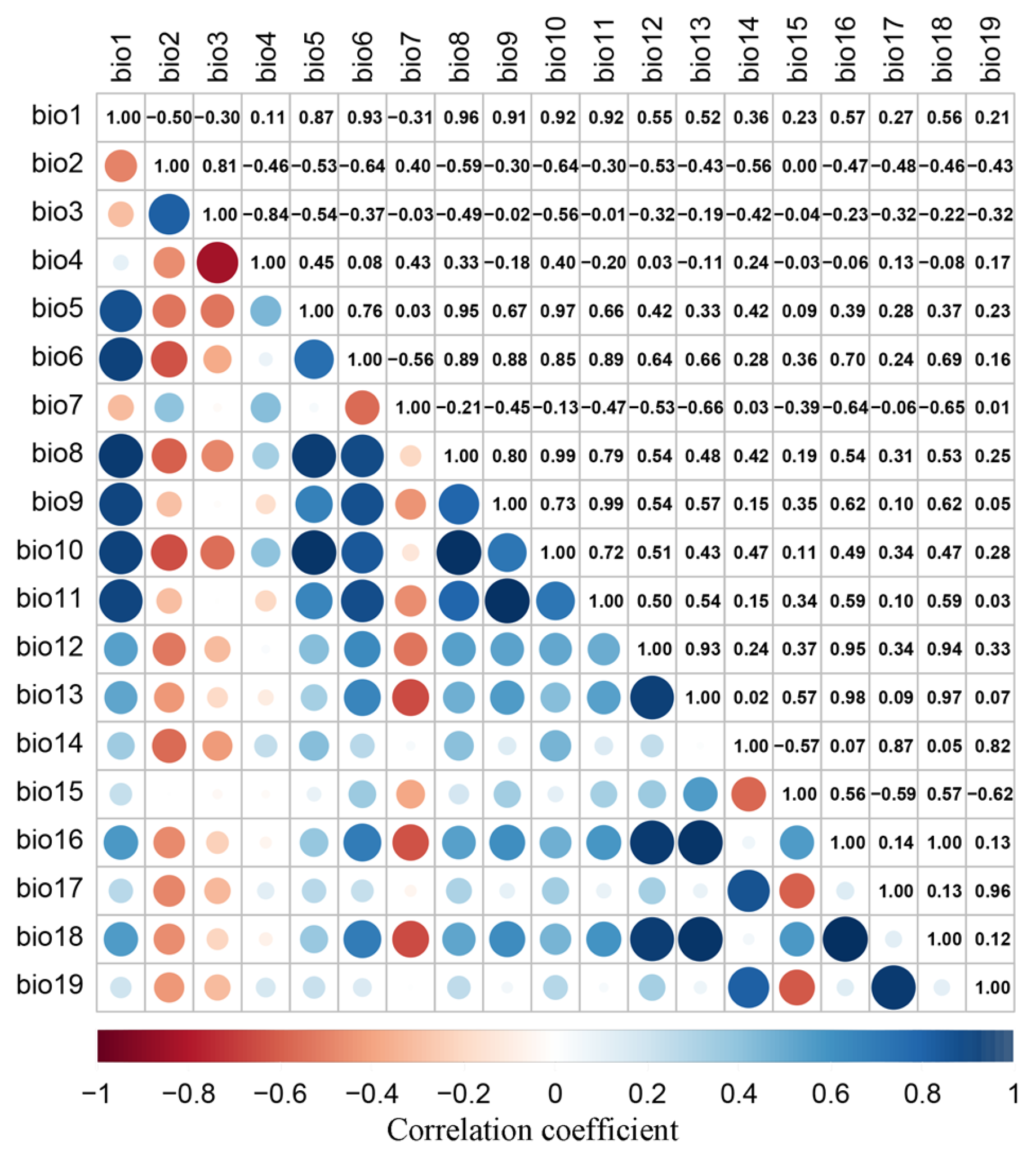
2.3. Acquisition of Environmental Variables

In selecting environmental variables for modeling, we used only climate-related data, excluding soil, human disturbance, topography, etc., for the following reasons: Firstly, using too many types of environmental factors in modeling can diminish the impact of climatic factors. Secondly, during the LGM, there was no human disturbance, and the soil and vegetation conditions were different from the present. Additionally, the model’s depiction of the relationship and niche between climate, disturbance, topography, soil, and vegetation may not be transferable in terms of spatial and temporal scales, whereas only climatic factors possess transferability. The climatic data required for our study were downloaded from the WorldClim database (http://www.worldclim.org/ (accessed on 21 March 2023)). The latest iteration of the international Coupled Model Intercomparison Project (CMIP6) has released dozens of Global Climate Models (GCMs), each with varying predictive accuracies for different regions and bioclimatic variables (bio1–bio19). For our study, we utilized the WorldClim2.1 dataset, downloading bioclimatic variables from 1970–2000 for predicting the current distribution of L. pinceana under prevailing climatic conditions. Additionally, we downloaded data from four GCMs with strong predictive capabilities for temperature and precipitation in China, the Centre National de Recherches Météorologiques Model Version 6 (CNRM-CM6-1), the European Community Earth System Model version 3 with Vegetation (EC-Earth3-Veg), the Euro-Mediterranean Center on Climate Change Earth System Model Version 2 (CMCC-ESM2), and the coupled Max Planck Institute Earth System Model version 1.2 in a higher-resolution configuration (MPI-ESM1-2-HR) [50,51], for predicting the future distribution in the 2050s and 2090s. The EC-Earth3-Veg model, known for its accuracy and reliability in simulating complex dynamics of the climate system, was chosen for illustration in subsequent analyses [52]. Each GCM provides four shared socioeconomic pathway (SSP) scenarios, projecting different climate change outcomes under varied socioeconomic development paths: SSP126 represents a sustainable development trajectory with a global average warming of 3 °C by 2100; SSP245 indicates a moderate development pathway, following a trend consistent with historical patterns with a global average warming of 3.7 °C by 2100; SSP370 suggests a regional rivalry development pathway with a global average warming of 4.1 °C by 2100; and SSP585 depicts a high-speed development pathway with a global average warming of 5.1 °C by 2100 [14,41]. Since paleoclimate data from WorldClim2.1 were not yet available, we used Community Climate System Model version 4 (CCSM4) from the WorldClim1.4 dataset, developed by the National Center for Atmospheric Research to better simulate East Asian climate characteristics [49], for predictions during the LGM and the MH periods. We scaled down the temperature layer values to one tenth of their original to maintain consistency with current and future layer units [14].
Before modeling, it was essential to filter the environmental variables: we repeatedly ran a single initial model in the Biomod2 five times and integrated models with an Area Under the Receiver Operating Characteristic Curve (AUC-ROC/AUC) greater than 0.8 to calculate the contribution rate of each climatic variable. Variables contributing less than 2% were eliminated [24,53], leading to the exclusion of the mean temperature of wettest quarter (bio8) and the variation in precipitation seasonality (bio15). To prevent model overfitting due to multicollinearity among environmental variables, we conducted a correlation analysis (Figure 2) after extracting the environmental data for the distribution points using ArcGIS 10.4. Variables with a Spearman correlation coefficient greater than 0.7 and with lesser biological significance were discarded. We retained the mean diurnal range (bio2), the isothermality (bio3), the variation in temperature seasonality (bio4), the minimum temperature of coldest month (bio6), the temperature annual range (bio7), the mean annual precipitation (bio12), the precipitation of wettest month (bio13), the precipitation of warmest quarter (bio18), and the precipitation of coldest quarter (bio19). Subsequently, we removed variables with a Variance Inflation Factor (VIF) greater than 10, until all remaining variables had VIF values below 10 [9,24] (Table 1). Ultimately, six climatic factors were obtained for subsequent modeling work. All environmental variable layers used in this study were processed in ArcGIS 10.4, extracting the China region, and standardized to a 2.5′ resolution in TIFF format with the WGS 1984 coordinate system.

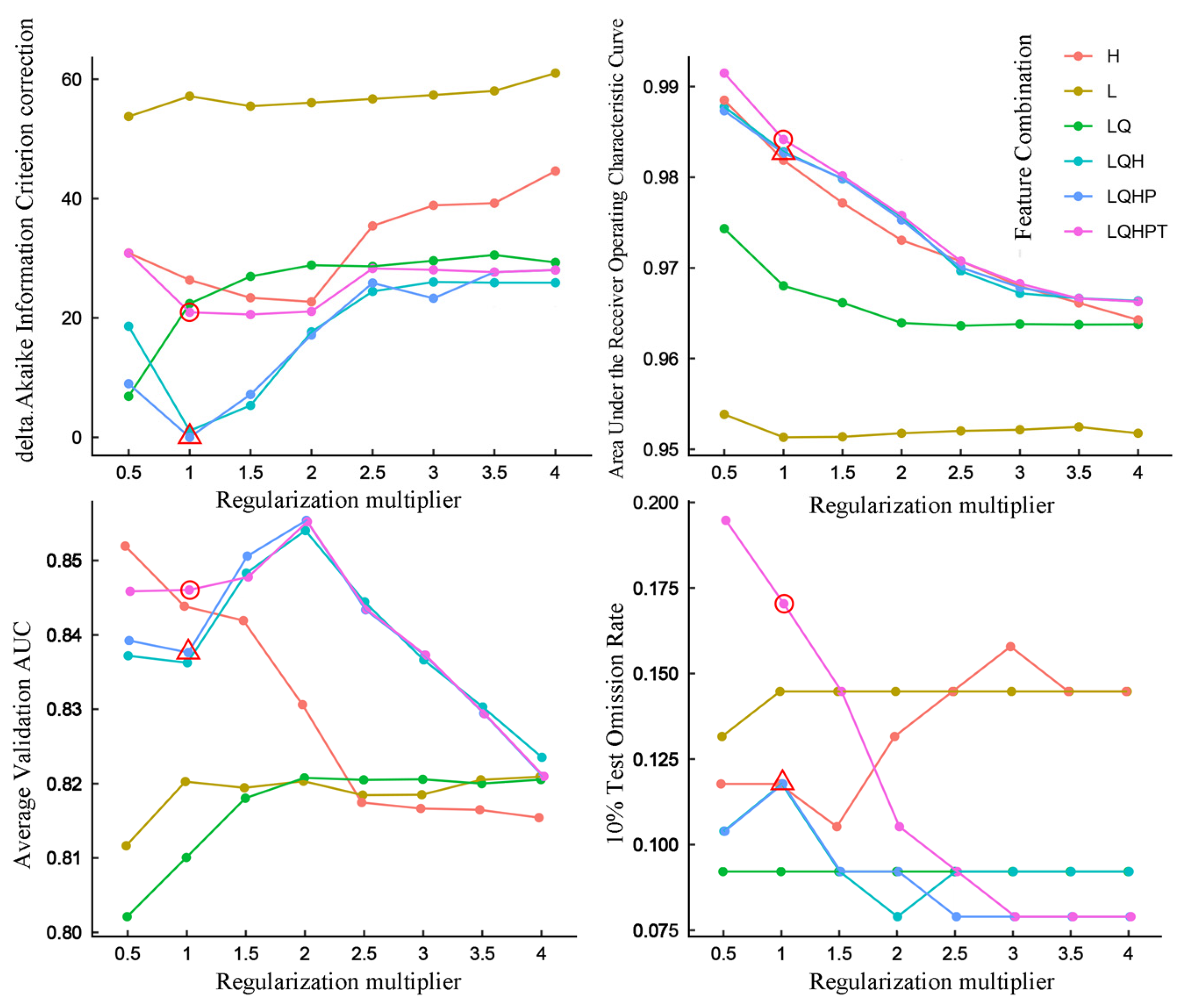
2.4. Model Evaluation and Construction

For model construction, we predominantly utilized the Biomod2 and ENMeval2.0 packages within R. Our evaluation encompassed a diverse range of SDMs, including Generalized Linear Models (GLMs), Generalized Boosted Models (GBMs), Generalized Additive Models (GAMs), Classification Tree Analysis (CTA), Artificial Neural Network (ANN), one Rectilinear Envelope Similar to BIOCLIM (SRE), Flexible Discriminant Analysis (FDA), Multivariate Adaptive Regression Splines (MARS), Random Forest (RF), and Maximum Entropy Models (MaxEnt). Initially, we optimized key parameters of MaxEnt using the ‘ENMeval2.0’ package: setting a range for the Regularization Multiplier (RM) from 0.5 to 4 at intervals of 0.5, and combining the five features of MaxEnt (linear (L), quadratic (Q), hinge (H), product (P), threshold (T)) into six Feature Combinations (FCs) [54]. We set 500 random background points and ran MaxEnt 48 times with RM and FC parameter combinations, subsequently calculating evaluation metrics for each combination: Akaike Information Criterion correction (AICc), AUC, Average Validation AUC (AUC.val.avg), and 10% Test Omission Rate (OR10). Lower delta.AICc values indicate better model performance [14], with AUC values between 0 and 1: values above 0.95 suggest excellent performance, those between 0.90 and 0.95 indicate good performance, those between 0.80 and 0.90 suggest fair performance, and those below 0.80 indicate poor performance [55]. AUC.val.avg, reflecting the MaxEnt model’s prediction accuracy across multiple validations, provides an average AUC value, with higher values indicating greater accuracy in predicting unknown data. OR10 assesses the model’s fit to distribution points [56].
After optimizing MaxEnt parameters, we used Biomod2 to construct ten single models and one Full Ensemble Model (FEM) using default parameters. Simultaneously, we built an optimized MaxEnt.2 model using RM and FC values corresponding to delta.AICc = 0. The ‘metric.eval’ command in Biomod2 was used to output True Skill Statistic (TSS), AUC, and kappa coefficient (kappa) for model accuracy evaluation. We then constructed an Optimal Ensemble Model (OEM) from models with TSS > 0.80 [41,57], AUC > 0.95, and good kappa performance [55,58]. After individually evaluating each single and combined model, we used the highest-accuracy model for subsequent predictions of suitable patterns and to output significant environmental factor results. In our modeling process, we generated 500 random background points [59], allocated 75% of distribution points as the training set and the remaining as the test set, and repeated the process five times [60,61].

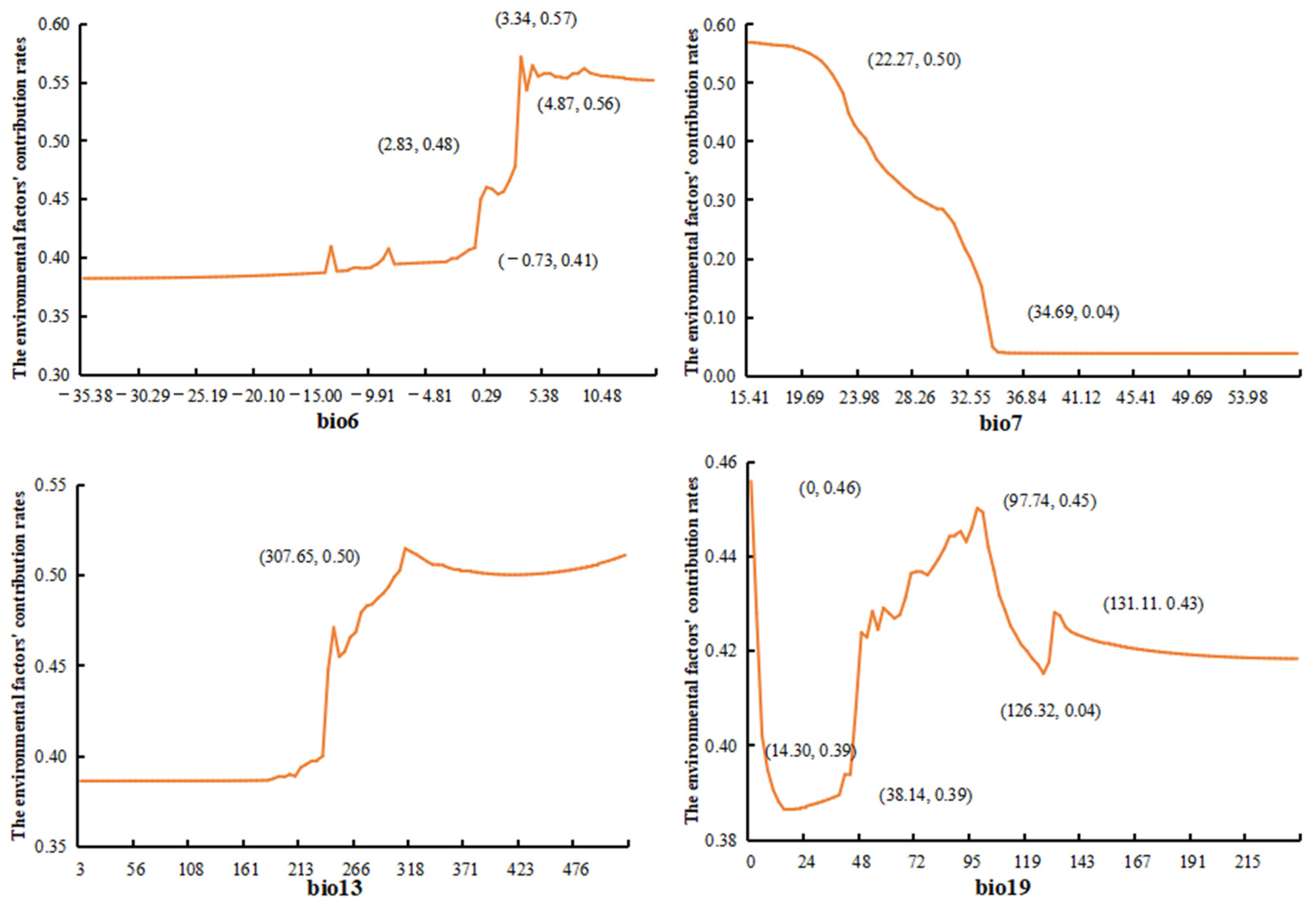
2.5. Analysis of Important Environmental Factors and Suitable Habitat Patterns

We employed the OEM to predict the current climate scenario and projected the results onto new scenarios to simulate past and future suitable conditions for L. pinceana, generating species distribution probability data. Utilizing the principle of maximizing the TSS, the threshold of maximum training sensitivity plus specificity was deemed the most accurate prediction method [62,63]. Therefore, we maximized TSS in the Biomod2 to create binary maps, converting the probability maps predicted by the OEM model into binary species distribution grid maps based on the threshold (AUC > 0.8). We used the ‘bm_PlotResponseCurves’ command to output response curve results for significant environmental factors and the ‘writeRaster’ command to produce grid files of suitable species distribution areas and binary maps of suitable/non-suitable habitats. Finally, we imported the suitability grid files into ArcGIS 10.4 and performed a normalization process on the grid values. Then, using the reclassification tool, we manually divided the suitability into four categories: no suitability (grid value = 0), low suitability (0 < grid value ≤ 0.4), medium suitability (0.4 < grid value ≤ 0.6), and high suitability (0.6 < grid value ≤ 1) [9]. These steps enabled us to obtain predictive maps of habitat distribution for different suitability levels. The binary maps were then used in the SDM toolbox v2.5 with the MaxEnt Tools plugin to calculate areas of contraction, expansion, and stability under different climatic scenarios, as well as centroid changes [64]. Finally, the analysis tools in ArcGIS 10.4 were used to calculate the centroid distance of suitable areas.

3. Results

3.1. Model Construction and Important Environmental Factors

Utilizing MaxEnt with default parameters (RM = 1, FC = LQHPT) resulted in a delta.AICc value of 20.927. However, parameter optimization, specifically using RM = 1 and FC = LQHP, reduced the delta.AICc to 0, indicating that this parameter setting yielded the best performance for MaxEnt under these conditions (Figure 3). The optimized MaxEnt model showed an AUC.val.avg of 0.838 and an AUC of 0.983, compared to the default AUC.val.avg of 0.846 and AUC of 0.984. Although both AUC.val.avg and AUC decreased slightly, the model’s accuracy remained high. Additionally, the OR10 value decreased from 0.170 in the default setting to 0.118, indicating a reduced fit between the distribution points and the model, hence a simpler optimized MaxEnt. After re-running the single models five times, we found that the evaluation metrics for MaxEnt.2 were higher than before optimization. Consequently, we selected the high-performing models GLM, GBM, FDA, MARS, RF, and MaxEnt.2 for constructing the OEM (Table 2). Upon comparing each model’s evaluation metrics, we found that OEM had the highest TSS and AUC, 0.919 and 0.982, respectively, and a kappa value of 0.822, second only to RF’s 0.831. The overall performance of the OEM model was best; hence, it was chosen for subsequent analysis of L. pinceana’s suitable habitat patterns. In our model evaluation process, all the assessment indicators performed well. Similar results can be found in studies on Eucalyptus grandis [55] and Abies spp., Pinaceae [58].
The model sensitivity to each environmental variable differs, with six climatic factors impacting L. pinceana’s geographic distribution patterns to varying extents (Figure 4). Among the results of the environmental factors’ contribution rates, the temperature annual range (bio7) and the minimum temperature of the coldest month (bio6) have the greatest impact on L. pinceana, followed by the precipitation of the wettest month (bio13). However, the response curves for the precipitation of the coldest quarter (bio19), the mean diurnal range (bio2), and the variation in temperature seasonality (bio4) show significant fluctuations, but the overall suitability remains below 0.5, having a relatively minor impact on the survival of L. pinceana. The survival probability of L. pinceana is higher when bio7 is less than 22.27 °C; beyond this value, the survival rate noticeably decreases. When the temperature annual range exceeds 34.69 °C, the survival rate of L. pinceana almost drops to zero and remains unchanged thereafter. L. pinceana tolerates bio6 within the range of 2.83–3.34 °C. Below 2.83 °C, the survival rate declines, and at temperatures below freezing (−0.73 °C), the suitability remains at a lower level. Above 3.34 °C, it generally remains at a higher level. The survival of L. pinceana is most favorable when the bio13 exceeds 307.65 mm.

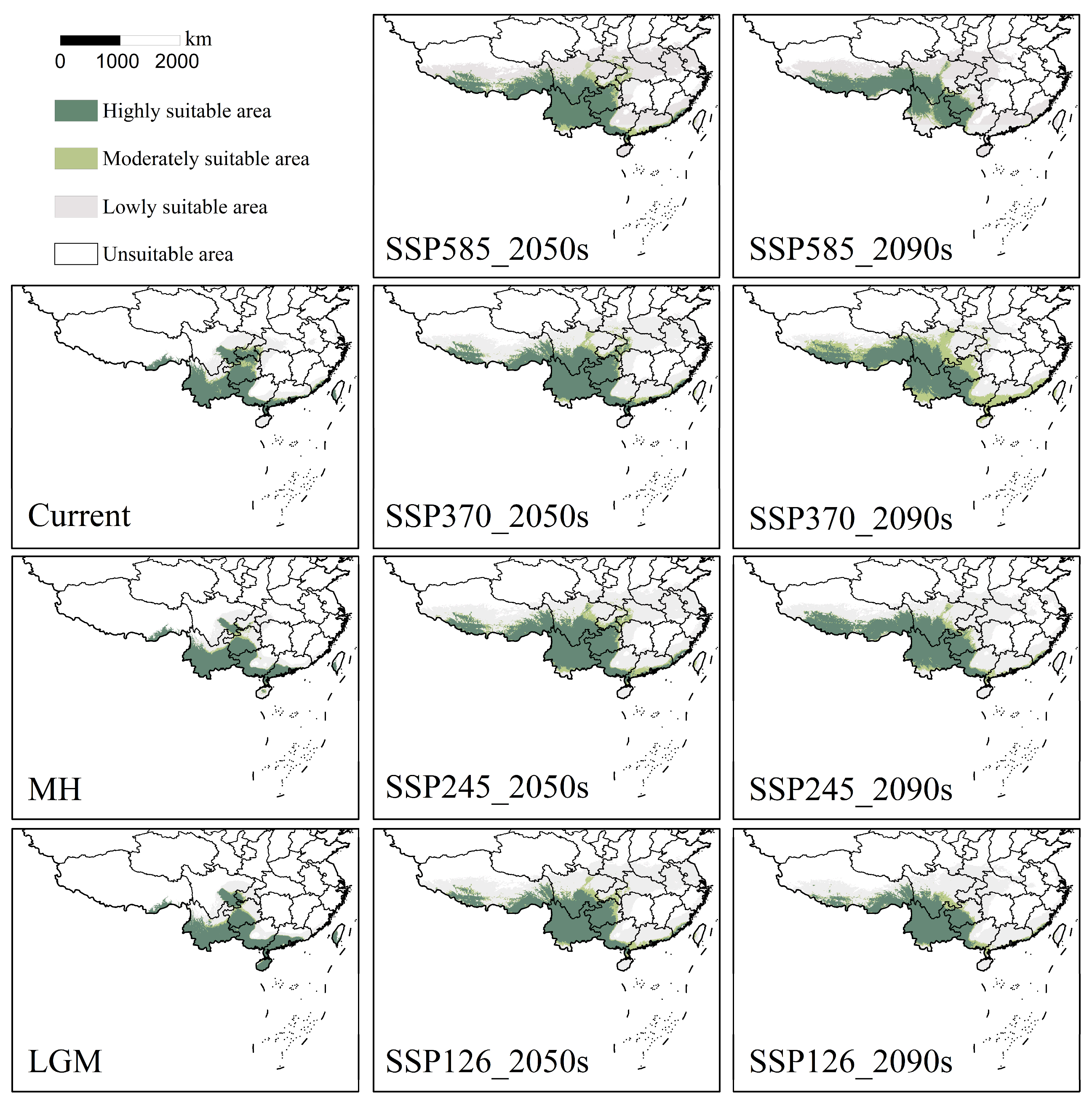
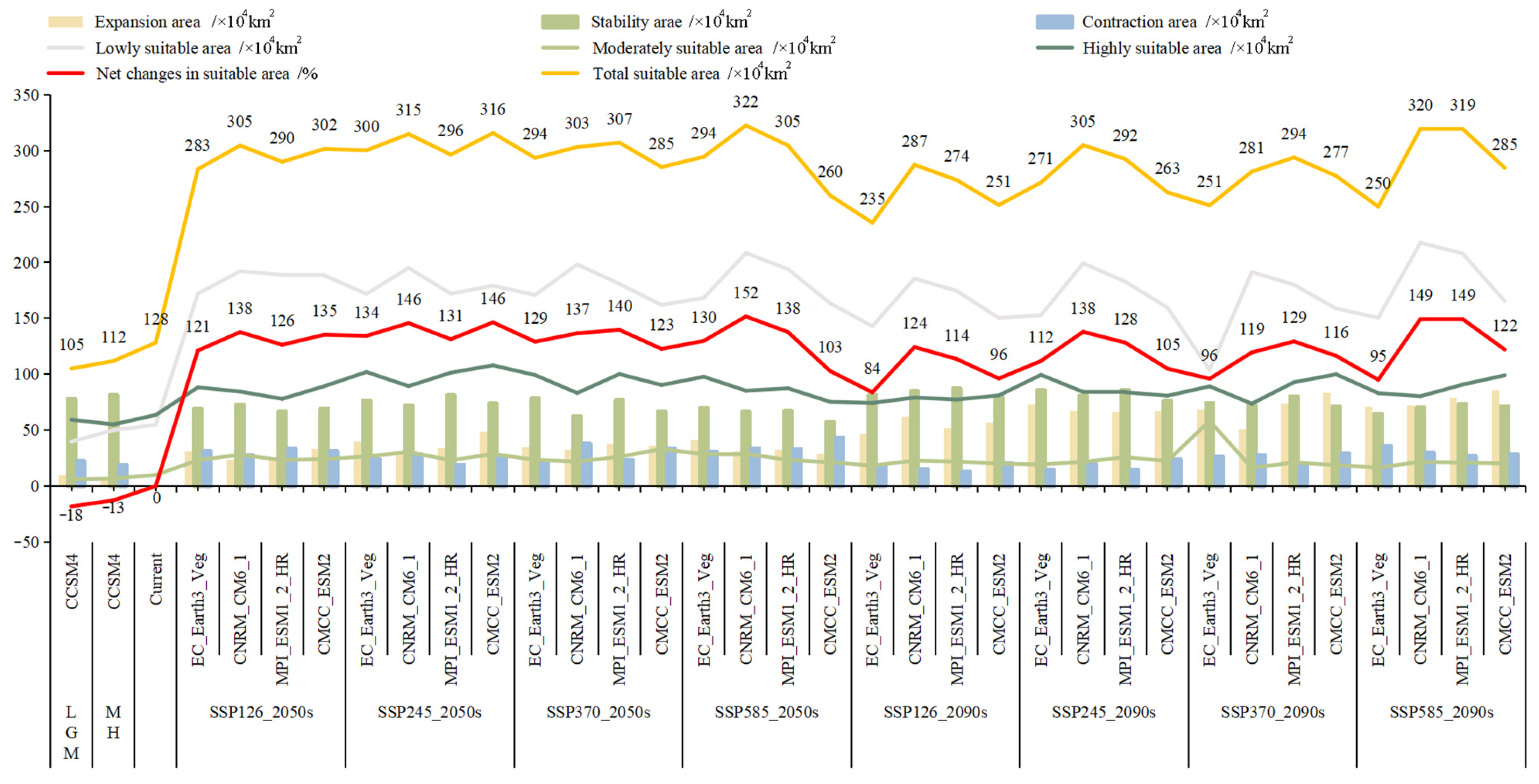
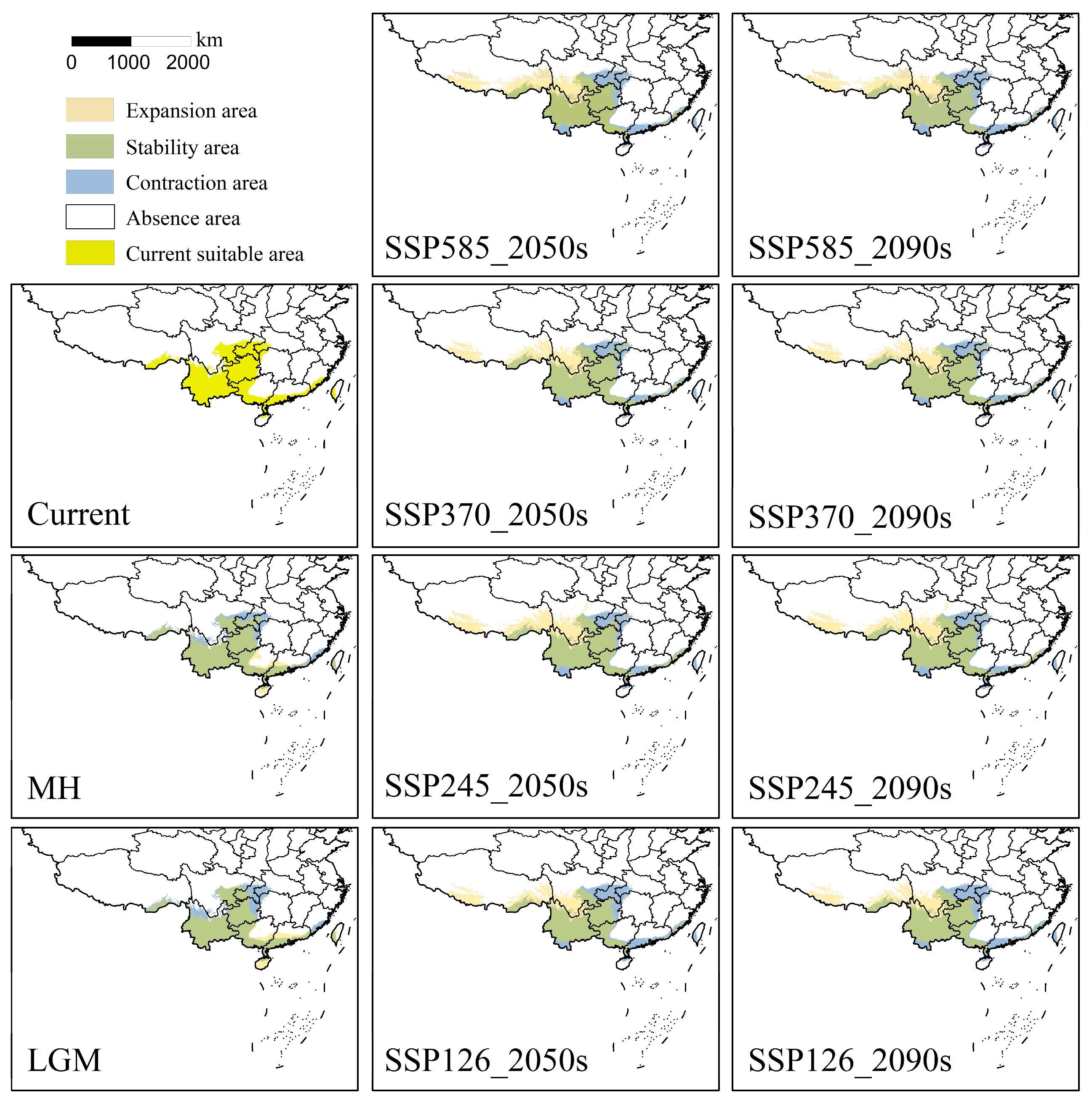
3.2. Analysis of Suitable Area Patterns

Under the current climatic scenario, the total suitable area for L. pinceana in China was estimated to be 128 × 104 km2, with a highly suitable area spanning 64 × 104 km2, primarily in most regions of Yunnan and Guizhou provinces, and the western part of Guangxi Zhuang Autonomous Region. Additionally, southwestern Sichuan Province, southern Chongqing, and the southern border of Linzhi in the Tibet Autonomous Region also constituted the medium and highly suitable areas. The coastal areas of southern China, along with Hainan and Taiwan provinces, were also identified as suitable for L. pinceana (Figure 5). The potential distribution areas during the LGM and the MH periods were largely consistent with the current distribution pattern, with L. pinceana’s suitable habitats predominantly stable in Southwest China. However, under paleoclimate conditions, the eastern coastal areas showed a more extensive and higher suitability, with most of Hainan province being highly suitable for L. pinceana during the LGM (Figure 6). The net change in the suitable area for L. pinceana from the MH to the present indicated a decrease of 13%, with the total suitable area reducing by 16 × 104 km2. The change from the LGM to the MH was even less (Figure 7), primarily shifting towards the northwest (Figure 7, Figure 8 and Figure 9). By the end of this century, although the climate will continue to change L. pinceana’s suitable patterns, two regions will consistently remain highly suitable: The first is in northwestern Yunnan, including Dali Bai Autonomous Prefecture, Nujiang Lisu Autonomous Prefecture, Baoshan City, Dehong Dai and Jingpo Autonomous Prefecture, the western part of Lijiang City, and the southern part of Diqing Tibetan Autonomous Prefecture. The second is the contiguous area where Yunnan, Guizhou, and Guangxi meet, including Qujing City, Kunming City, Yuxi City, Wenshan Zhuang and Miao Autonomous Prefecture; the eastern part of Honghe Hani and Yi Autonomous Prefecture in Yunnan Province, Liupanshui City, Anshun City, Bijie City, Guiyang City, Qianxinan Buyei and Miao Autonomous Prefecture; and the western part of Qiannan Buyei and Miao Autonomous Prefecture in Guizhou Province, as well as Baise City and the northwestern part of Hechi City in Guangxi Zhuang Autonomous Region (Figure 6).
Figure 7 depicts the changes in the suitable area for L. pinceana as predicted by four Global Climate Models (GCMs). The results of L. pinceana’s suitable areas under different future climate scenarios show slight differences but generally fluctuate within a narrow range. Among these, the EC-Earth3-Veg and CMCC-ESM2 models produce more conservative results, while the CNRM-CM6-1 and MPI-ESM1-2-HR models predict larger suitable areas. From the LGM to the year 2100 (LGM–MH–Current–2050s–2090s), the overall suitable area of L. pinceana tends to migrate towards higher altitudes and latitudes (Figure 6), exhibiting a trend of ‘stability-expansion-expansion-contraction’ (Figure 7). Under the predictions of the four GCMs, two time periods, and four shared socioeconomic pathways, the total suitable area of L. pinceana is estimated to be between 235 and 322 × 104 km2, with the highly suitable area ranging from 74 to 108 × 104 km2 (Figure 7). The results of all four GCMs indicate a significant increase in the total suitable area of L. pinceana by the 2050s, with the lowly suitable area expanding eastward to encompass the entire South China region as well as the northern parts of Central and East China. Medium- and high-level suitable areas also show an increase compared to the present, with the greatest expansion seen in the lowly suitable area. By the 2090s, there will be a slight contraction in the suitable area of L. pinceana at different suitability levels, with Central and South China no longer being conducive to the growth of L. pinceana (Figure 6 and Figure 7). In the future, the net changes in the suitable area of L. pinceana are all positive, often exceeding one hundred, indicating that the future suitable area will double from the current climatic scenario. Overall, the future climate will be more favorable for the survival of L. pinceana.
In future climatic models, L. pinceana’s potential distribution areas in most parts of Yunnan and Guizhou provinces and the northwestern and coastal regions of Guangxi Zhuang Autonomous Region exhibit high stability. The suitable areas are predicted to expand northwestward, and with the progression of time and intensification of climatic trends, the changes in L. pinceana’s suitable habitats become more pronounced. This increase in suitability is particularly noticeable in the southern part of Sichuan Province and the Tibet Autonomous Region, while the suitability in Chongqing, Dazhou, and Guang’an cities in Sichuan Province, and Xishuangbanna Dai Autonomous Prefecture in Yunnan, as well as the eastern coastal regions of China, are expected to decline (Figure 8).

3.3. Analysis of Centroids Migration

Throughout the period from the LGM to the present, the centroids of the suitable habitat for L. pinceana have consistently been located in the Qianxinan Buyei and Miao Autonomous Prefecture, Guizhou Province. During the transition from the LGM to the MH, the centroids moved northwest by 58 km and then shifted 86 km northeast under the current climate conditions. Under different GCM predictions, the future migration trajectories of L. pinceana’s centroids are consistent, predominantly moving northwestward. Taking the EC-Earth3-Veg model’s predictions as an example, under future climatic scenarios, the centroids of L. pinceana primarily remain in the northwestern region of Yunnan Province. Under SSP126, by the 2050s, the centroid shifts 394 km west-northwest to Lijiang City, and by the 2090s, it moves northeast by 23 km, remaining in the same area. Under SSP245, the centroid moves 392 km northwest to Lijiang City by the 2050s and continues moving 87 km northwest, remaining within Lijiang City by the 2090s. Under SSP370, the centroid relocates 346 km to Panzhihua City, Sichuan Province, by the 2050s, and by the 2090s, it shifts another 180 km northwest to Diqing Tibetan Autonomous Prefecture, Yunnan Province. Under SSP585, by the 2050s, the centroid moves 460 km to Lijiang City, and by the 2090s, it migrates 170 km northwest to Diqing Tibetan Autonomous Prefecture (Figure 9).
Across four GCMs, the centroids of L. pinceana’s suitable habitat in the 2050s consistently show a northwestward movement towards the junction of Lijiang City and Panzhihua City. By the 2090s, under SSP126, the centroid moves the least and is the only trajectory heading northeast. Under the other three pathways, the centroids continue to move northwest, with the migration distance increasing as the socioeconomic development scenarios become more severe. A comprehensive analysis reveals that with future climatic changes, the centroids of L. pinceana’s suitable habitat tend to move towards higher altitudes and latitudes in the northwest direction (Figure 9).

4. Discussion

4.1. Application and Limitations of SDMs

SDMs are statistical or inferential models developed based on niche theory. They play a crucial role in predicting the potential geographic distribution of species by analyzing the complex relationships between species and their environments. SDMs serve as vital tools in ecology, biogeography, and evolutionary biology, guiding species conservation and practical management actions [34,46,49]. One of the main challenges in constructing species distribution models is choosing appropriate model algorithms and parameter settings [34], which is a complex and critical step that requires a comprehensive consideration of the species’ ecological traits and environmental adaptability [65]. Nearly two decades ago, Elith et al. [66] compared various SDMs, among which MaxEnt stood out due to its ease of use and high accuracy in simulation, rapidly surpassing other SDMs in terms of usage rate over the following years [43]. However, while optimizing key parameters in MaxEnt can effectively enhance model accuracy [14], it is not necessarily the optimal solution. During our use of Biomod2, we found that the optimally enhanced MaxEnt model, although showing improved evaluation metrics, was outperformed by the OEM integrated from exceptionally performing single models such as GLM, GBM, FDA, MARS, RF, and MaxEnt.2. This OEM more accurately simulated the shift in suitable areas for L. pinceana under climate change. In the process of species distribution modeling, factors such as species characteristics, accuracy of distribution points, selection of environmental variables, and differences in parameter configuration can affect the model’s precision and applicability [67]. Therefore, when conducting such research, it is advisable not to blindly choose SDMs but rather to compare multiple models to select the most suitable one. Although the AUC is a commonly used metric for evaluating model performance, its reliability is limited when used alone [68]. We employed multiple evaluation metrics to comprehensively assess model performance, using models with TSS > 0.80, AUC > 0.95, and good kappa performance for integrated prediction. This multidimensional assessment significantly enhanced the reliability and effectiveness of the predictions. Such an approach not only avoids the limitations of single-metric evaluation but also provides a more comprehensive perspective for assessing overall model performance, thereby increasing confidence in species distribution prediction work [35].
Plants possess a certain level of adaptability to their environment, and changes in living conditions brought about by climate change can impact this adaptability [1]. Understanding how plants survive and reproduce under dynamic climatic conditions is crucial. Additionally, the scale of research can affect the predictive outcomes of SDMs. Studies on ornamental plants in China, for example, have shown that regional scales (such as Taizhou City and Southeast China) predict a larger suitable range than when using a national scale [63]. Moreover, the scale of this study influences the model’s determination of dominant environmental factors. Our research was conducted at the national scale for China, without incorporating the adaptability and migration capabilities of plants. In future studies, it is advisable to conduct research at regional scales to compare the model’s response to different environmental factors. On the other hand, further exploration is needed on how to integrate ecological and physiological factors into the model considerations [46].

4.2. Geographical Distribution Changes of L. pinceana

After running the OEM five times consecutively, the average values of the Area Under the Receiver Operating Characteristic Curve (AUC) and TSS were found to be above 0.9, indicating an extremely high reliability of the model results. These can be used to explore the response of L. pinceana to climate change in terms of suitable habitat conditions. From the LGM to the year 2100, although the total suitable area of L. pinceana during the LGM was smallest, the changes in suitable area and centroids between the LGM, the MH, and the current period were relatively minimal. There was only a slight contraction and southward shift from the LGM to the present, consistent with the behavior of Tsoongiodendron odorum during the LGM as studied by Hu et al. [5]. Despite the dry and cold climate of the Pleistocene ice age leading to significant changes in the geographic distribution of many plants [5,69], and the substitution of tropical vegetation by subtropical evergreen broadleaf forests in China, instances of plants taking refuge in situ were not uncommon [14,70]. L. pinceana primarily inhabits monsoon rainforests, rainforest regions, and subtropical evergreen broadleaf forest zones. Highly suitable areas involve regions with strong topographic heterogeneity, such as the Wuliang Mountains, Ailao Mountains, Jingmai Mountains, Wumeng Mountains, and the Sichuan Basin in Yunnan. Therefore, it is speculated that L. pinceana might have been preserved in microenvironments of mountainous areas during the LGM.
By the MH period, the suitability of L. pinceana in provinces such as Guangdong, Hainan, and Taiwan gradually diminished, likely related to the melting of ice caps and intensified temperature changes following the LGM. This led to an inland migration of L. pinceana’s suitable habitats, a phenomenon consistent with its family relative, Emmenopterys henryi [9]. The post-glacial migrations have profoundly impacted the population structures of many plant species, playing a significant role in shaping contemporary genetic variation patterns in several taxa within Southwest China [71]. Having undergone continual changes and adaptations, L. pinceana has developed unique genetic variation patterns, which are of substantial importance for its survival and reproduction. From the MH to the 2050s, the total suitable area of L. pinceana experienced two increases, primarily manifested as a surge in the area of lowly suitable habitats, with large lowly suitable areas emerging in the eastern regions over time. This increase is likely due to rising surface temperatures expanding L. pinceana’s habitable environments [72]. However, these expansions of L. pinceana’s suitable areas contrast with the habitat changes of E. henryi [9], possibly due to differences in the ecological traits of the two species, with the relict plant E. henryi being more sensitive to climate. Regardless of future climatic changes, L. pinceana’s suitable habitats remain within the subtropical monsoon climate zone, concentrated in Southwest China. Currently, L. pinceana’s suitable habitats have not reached saturation, and its survival does not require protection yet. Nevertheless, the outlook for L. pinceana is not entirely optimistic. After peaking in the 21st century, the suitable area for L. pinceana is expected to decrease again by the 2090s, with the possibility of continued reduction in suitable habitat areas. With future human activities contributing to rising atmospheric temperatures and increasing frequencies of extreme climate events [9], the centroids of L. pinceana’s suitable area will move significantly northwestward. By the end of the 21st century, L. pinceana’s suitable areas in eastern cities will significantly diminish, while the suitable areas in the Tibet Autonomous Region and Sichuan Province will expand, and the more severe the climate change, the more pronounced the changes in suitable area. This reaffirms that climate can alter the geographic distribution patterns of plants, even changing plant diversity at the regional level [15]. In the future, L. pinceana’s highly suitable areas will mainly be in Yunnan Province and adjacent areas, with the total suitable area continuously moving towards the plateau. The impact of climate change on the distribution and extent of species’ suitable habitats is a core issue in biodiversity research. Studies by Zhang et al. [73] and Zhou et al. [74] have highlighted how climate change leads to changes in species distribution patterns and habitat fragmentation, which align with the changes in L. pinceana’s suitable habitats observed in this study.

4.3. Analysis of Key Climatic Factors for L. pinceana

The temperature annual range (bio7), the minimum temperature of the coldest month (bio6), and the precipitation of the wettest month (bio13) are the dominant climatic factors affecting the distribution of L. pinceana, with bio7 having the most significant impact. Research by Ma et al. [75] comparing the effects of climatic, topographic, and soil environmental factors on the distribution patterns of major tree species in Southwest China found that thermohydrodynamic conditions are the dominant environmental factors affecting richness patterns, with a more pronounced response to temperature. The geographic distribution of plants at a regional scale is primarily influenced by climate, especially thermohydric conditions, as numerous studies in the Himalayan region have shown that temperature plays a vital role in determining the habitat distribution of species [2,24,47]. L. pinceana, a characteristic plant to Southwest China, predominantly inhabits warm and humid areas, explaining its strong response to temperature and precipitation.
Environmental changes can also increase the risk of invasion by ornamental exotic plants [63]. China, with its rich germplasm resources, benefits from protecting native plants for ecosystem stability. L. pinceana, a plant of Southwest China with both ornamental and medicinal values, faces reduced survival pressure in the future compared to the present. Subsequent efforts can focus on strengthening the introduction and artificial breeding of L. pinceana to enhance the application value of its resources. Our work provides insights into assessing the impact of climate change on the distribution of L. pinceana, aiding in understanding how native plants like L. pinceana in Yunnan respond to future climate changes. This can offer theoretical references for the conservation and effective utilization of L. pinceana’s wild resources.

5. Conclusions

Utilizing the effective distribution data of L. pinceana and a set of environmental variables, we have developed an Optimal Ensemble Model. This model reveals that the temperature annual range (bio7), the minimum temperature of the coldest month (bio6), and the precipitation of the wettest month (bio13) are the key environmental factors shaping the distribution pattern of L. pinceana. This species exhibits a significant requirement for the environmental requirements for precipitation and temperature, with a particular sensitivity to temperature during its growth and development phases. Historically, in the LGM, L. pinceana demonstrated a widespread and continuous distribution across the tropical and subtropical southern regions of China. By the MH, although the overall suitable area remained relatively unchanged, the suitability in the eastern coastal regions experienced a decline. Presently, under the existing climatic conditions, there is an observed expansion in the suitable area for L. pinceana, predominantly in Southwest China. Looking ahead, it is anticipated that the suitable area for L. pinceana will continue to expand in response to the ongoing increase in temperatures. By the end of the 21st century, the areas most conducive to its growth are expected to shift towards higher latitudes and elevations.
This research is focused on analyzing the distribution patterns of L. pinceana within China. Future investigations could extend to a global perspective, examining the geographical distribution patterns of the five species within the genus Luculia. This would involve conducting cluster analyses of habitat preferences at the genus level and assessing the phylogenetic relationships among these species. Our findings offer scientific guidance for the conservation and utilization of wild resources of L. pinceana in China. Given the analogous habitat preferences identified among the five species within the genus Luculia, subsequent studies should delve into understanding the niche similarities and the phylogenetic connections among different species at the genus level. Such exploration will enhance our comprehension of the ecological adaptability and evolutionary dynamics of L. pinceana. Furthermore, we acknowledge that not employing downscaling techniques in this study may have implications for the local applicability of our results. Despite this, the methods and data we utilized have effectively revealed the primary environmental drivers of L. pinceana distribution patterns. In future research, it could be planned to implement downscaling techniques to enhance the precision and regional applicability of the models. This will aid in a more detailed assessment of the impacts of climate change on the distribution of L. pinceana, providing a more accurate scientific basis for its conservation and utilization.

Author Contributions

Conceptualization, C.G. and C.M.; methodology, S.G.; software, R.L.; validation, X.K. and J.Y.; formal analysis, S.G.; investigation, C.G.; resources, C.M.; data curation, J.Y.; writing—original draft preparation, C.G.; writing—review and editing, C.G. and C.M.; visualization, C.G. and S.G.; supervision, C.M.; project administration, C.M. All authors have read and agreed to the published version of the manuscript.

Funding

This research was funded by the Yunnan Province Department of Education Science Research Fund Project, China (grant numbers 2023Y0743 and 2023Y0757). This work was supported by the Joint Special Project on Basic Agricultural Research in Yunnan Province, China (grant numbers 202101BD070001-100 and 202301BD070001-150). This research was supported by the Key Laboratory of Forest Resources Conservation and Utilization in the Southwest Mountains of China Ministry of Education, Southwest Forestry University, China (grant numbers LXXK-2023M05).

Data Availability Statement

The data that support the findings of this study are available from the first author (C.G.) upon reasonable request.

Conflicts of Interest

The authors declare no conflicts of interest. The funders had no role in the design of the study; in the collection, analyses, or interpretation of data; in the writing of the manuscript; or in the decision to publish the results.

References

  1. Almeida, A.M.; Ribeiro, M.M.; Ferreira, M.R.; Roque, N.; Quintela-Sabarís, C.; Fernandez, P. Big data help to define climate change challenges for the typical Mediterranean species Cistus ladanifer L. Front. Ecol. Evol. 2023, 11, 1136224. [Google Scholar] [CrossRef]
  2. Wang, X.F.; Duan, Y.X.; Jin, L.L.; Wang, C.Y.; Peng, M.C.; Li, Y.; Wang, X.H.; Ma, Y.F. Prediction of historical, present and future distribution of Quercus sect. Heterobalanus based on the optimized MaxEnt model in China. Acta Ecol. Sin. 2023, 43, 6590–6604. [Google Scholar] [CrossRef]
  3. Zhang, A.P.; Wang, Y.; Xiong, Q.L.; Wu, X.G.; Sun, X.M.; Huang, Y.M.; Zhang, L.; Pan, K.W. Distribution changes and refugia of three spruce taxa since the last interglacial. Chin. J. Appl. Ecol. 2018, 29, 2411–2421. [Google Scholar] [CrossRef]
  4. Liu, D.T.; Chen, J.Y.; Sun, W.B. Distributional responses to climate change of two maple species in southern China. Ecol. Evol. 2023, 13, e10490. [Google Scholar] [CrossRef] [PubMed]
  5. Hu, W.; Zhang, Z.Y.; Chen, L.D.; Peng, Y.S.; Wang, X. Changes in potential geographical distribution of Tsoongiodendron odorum since the Last Glacial Maximum. Chin. J. Plant Ecol. 2020, 44, 44–55. [Google Scholar] [CrossRef]
  6. Ni, J.; Yu, G.; Harrison, S.P.; Prentice, I.C. Palaeovegetation in China during the late Quaternary: Biome reconstructions based on a global scheme of plant functional types. Palaeogeogr. Palaeoclimatol. Palaeoecol. 2010, 289, 44–61. [Google Scholar] [CrossRef]
  7. Tian, Z.P.; Jiang, D.B. Mid-Holocene and last glacial maximum changes in monsoon area and precipitation over China. Chin. Sci. Bull. 2015, 60, 400–410. [Google Scholar] [CrossRef]
  8. Zou, X.; Peng, Y.; Wang, L.; Li, Y.; Zhang, W.X.; Liu, X. Impact of climate change on the distribution pattern of Malus baccata (L.) Borkh. in China since the Last Glacial Maximum. Plant Sci. J. 2018, 36, 676–686. [Google Scholar] [CrossRef]
  9. Tang, Z.H.; Liu, X.A.; Peng, P.H.; Li, X.Y. Prediction of potential geographical distribution patterns of Emmenopterys henryi since the Last Glacial Maximum. Acta Ecol. Sin. 2023, 43, 3339–3347. [Google Scholar] [CrossRef]
  10. Shi, X.W.; Zhang, L.; Zhang, J.J.; Ouyang, Z.Y.; Xiao, Y. Priority area of biodiversity conservation in Southwest China. Chin. J. Ecol. 2018, 37, 3721–3728. [Google Scholar] [CrossRef]
  11. Fraga, H.; Molitor, D.; Leolini, L.; Santos, J.A. What is the impact of heatwaves on European viticulture? A modelling assessment. Appl. Sci. 2020, 10, 3030. [Google Scholar] [CrossRef]
  12. Dagtekin, D.; Şahan, E.A.; Denk, T.; Köse, N.; Dalfes, H.N. Past, present and future distributions of Oriental beech (Fagus orientalis) under climate change projections. PLoS ONE 2020, 15, e0242280. [Google Scholar] [CrossRef]
  13. Intergovernmental Panel on Climate Change. Climate Change 2013: The Physical Science Basis. Contribution of Working Group I to the Fifth Assessment Report of the Intergovernmental Panel on Climate Change; Cambridge University Press: Cambridge, UK, 2014. [Google Scholar]
  14. Fan, Z.F.; Zhou, B.J.; Ma, C.L.; Gao, C.; Han, D.N.; Chai, Y. Impacts of climate change on species distribution patterns of Polyspora sweet in China. Ecol. Evol. 2022, 12, e9516. [Google Scholar] [CrossRef]
  15. Boisvenue, C.; Running, S.W. Impacts of climate change on natural forest productivity—Evidence since the middle of the 20th century. Glob. Chang. Biol. 2006, 12, 862–882. [Google Scholar] [CrossRef]
  16. Wang, X.Y.; Chen, Y.; Yi, Y. Features of floral odor and nectar in the distylous Luculia pinceana (Rubiaceae) promote compatible pollination by hawkmoths. Ecol. Evol. 2023, 13, e9920. [Google Scholar] [CrossRef]
  17. Liu, X.X.; Ma, H.; Wan, Y.M.; Zhao, Z.G.; Li, Z.H. A new Luculia pinceana cultivar ‘Jinyudian’. Acta Hortic. Sin. 2019, 46, 199–200. [Google Scholar] [CrossRef]
  18. Ma, H.; Zhang, X.J.; Wan, Y.M.; Liu, X.X.; Li, Z.H. Breeding of a New Luculia gratissima Cultivar ‘Xiangbo’. N. Hortic. 2021, 45, 179–180. [Google Scholar] [CrossRef]
  19. Ma, H.; Wan, Y.M.; Liu, X.F.; Liu, X.X.; Li, Z.H. ‘Xianghun’, a New Luculia Hybrid Cultivar. Acta Hortic. Sin. 2020, 47, 3097–3098. [Google Scholar] [CrossRef]
  20. Li, Y.Y.; Xu, H.Y.; Ma, H.; Li, Z.H. Temporal variation of floral scent emission of a hybrid variety of Luculia. J. Shanxi Agric. Univ. 2020, 40, 8. [Google Scholar] [CrossRef]
  21. Li, Y.Y.; Wan, Y.M.; Sun, Z.H.; Li, T.Q.; Liu, X.F.; Ma, H.; Liu, X.X.; He, R.; Ma, Y.; Li, Z.H. Floral scent chemistry of Luculia yunnanensis (Rubiaceae), a species endemic to China with sweetly fragrant flowers. Molecules 2017, 22, 879. [Google Scholar] [CrossRef] [PubMed]
  22. Kang, W.Y.; Zhang, L.; Song, Y.L. α-Glucosidase inhibitors from Luculia pinciana. China J. Chin. Mater. Medica 2009, 34, 406–409. [Google Scholar]
  23. Li, H.Y.; Li, S.F.; Li, Y.F.; Kong, L.F. Study of Preservative Technology of Fresh Cut Flowers of Luculia pinceana. J. Dali Univ. 2023, 8, 96–100. [Google Scholar] [CrossRef]
  24. Sharma, M.K.; Ram, B.; Chawla, A. Ensemble modelling under multiple climate change scenarios predicts reduction in highly suitable range of habitats of Dactylorhiza hatagirea (D.Don) Soo in Himachal Pradesh, western Himalaya. S. Afr. J. Bot. 2023, 154, 203–218. [Google Scholar] [CrossRef]
  25. Bi, B.; Chen, Q.; Chang, E.F.; Li, P.R.; Yin, A.P. Phenological observation and value of ornamentation and utilization of Luculia intermedia. Guangxi For. Sci. 2005, 34, 135–136. [Google Scholar] [CrossRef]
  26. Kong, L.F.; Yang, Z.Y.; Li, S.F. Effect of low temperature stress on physiological effect and resistance induction on Luculia pinceana. Mol. Plant Breed. 2022, 20, 3069–3075. [Google Scholar] [CrossRef]
  27. Ma, H.; Wang, Y.; Li, Z.H.; Wan, Y.M.; Liu, X.X.; Liang, N. A study on the breeding system of Luculia pinciana. For. Res. 2009, 22, 373–378. [Google Scholar] [CrossRef]
  28. Chen, Y.; Wang, S.Y.; You, X.S.; Hu, D.M.; Yao, R.X.; Tang, X.X.; Wang, X.Y. A study of pollination accuracy in distylous Rubiaceae species (Luculia pinceana). Acta Ecol. Sin. 2021, 41, 6654–6664. [Google Scholar] [CrossRef]
  29. Li, Y.Y.; Ma, H.; Wan, Y.M.; Li, T.Q.; Liu, X.X.; Sun, Z.H.; Li, Z.H. Volatile organic compounds emissions from Luculia pinceana flower and its changes at different stages of flower development. Molecules 2016, 21, 531. [Google Scholar] [CrossRef] [PubMed]
  30. Li, L.; Wang, Q.; Xu, J. Application of integrated species distribution models in parasitic diseases prevention and control: A review. Chin. J. Schistosomiasis Control 2022, 34, 659–664. [Google Scholar] [CrossRef]
  31. Hutchinson, G.E. Concluding remarks. Cold Spring Harb. Symp. Quant. Biol. 1957, 22, 415–427. [Google Scholar] [CrossRef]
  32. Araújo, M.B.; Guisan, A. Five (or so) challenges for species distribution modelling. J. Biogeogr. 2006, 33, 1677–1688. [Google Scholar] [CrossRef]
  33. Chen, S.S.; Liu, X.; Tong, X.Y.; Guan, B.C. Prediction of Camellia edithae species distribution based on multi-model combination. Ecol. Sci. 2020, 39, 58–66. [Google Scholar] [CrossRef]
  34. Guo, Y.L.; Zhao, Z.F.; Qiao, H.J.; Wang, R.; Wei, H.Y.; Wang, L.K.; Gu, W.; Li, X. Challenges and development trend of species distribution model. Adv. Earth Sci. 2020, 35, 1292–1305. [Google Scholar] [CrossRef]
  35. Bai, J.J.; Hou, P.; Zhao, Y.H.; Xu, H.T.; Zhang, B. Research progress of species habitat suitability models and their verification. Chin. J. Ecol. 2022, 41, 1423–1432. [Google Scholar] [CrossRef]
  36. Zhu, G.P.; Liu, G.Q.; Bu, W.J.; Gao, Y.B. Ecological niche modeling and its applications in biodiversity conservation. Biodivers. Sci. 2013, 21, 90–98. [Google Scholar] [CrossRef]
  37. Han, J.L.; Williams, G.M.; Zou, Q.X.; Dong, B.N. The range and habitat suitability of François’ langur (Trachypithecus francoisi) in Mayanghe Nature Reserve, China. Environ. Sci. Pollut. Res. 2023, 30, 40952–40960. [Google Scholar] [CrossRef] [PubMed]
  38. Adão, F.; Campos, J.C.; Santos, J.A.; Malheiro, A.C.; Fraga, H. Relocation of bioclimatic suitability of Portuguese grapevine varieties under climate change scenarios. Front. Plant Sci. 2023, 14, 974020. [Google Scholar] [CrossRef]
  39. Fetene, E.; Teka, G.; Dejene, H.; Mandefro, D.; Teshome, T.; Temesgen, D.; Negussie, H.; Mulatu, T.; Jaleta, M.B.; Leta, S. Modeling the spatial distribution of Culicoides species (Diptera: Ceratopogonidae) as vectors of animal diseases in Ethiopia. Sci. Rep. 2022, 12, 12904. [Google Scholar] [CrossRef] [PubMed]
  40. Shi, Y.C.; Kang, B.; Fan, W.; Xu, L.L.; Zhang, S.M.; Cui, X.S.; Dai, Y. Spatio-temporal variations in the potential habitat distribution of Pacific sardine (Sardinops sagax) in the northwest Pacific Ocean. Fishes 2023, 8, 86. [Google Scholar] [CrossRef]
  41. Mallen-Cooper, M.; Rodríguez-Caballero, E.; Eldridge, D.J.; Weber, B.; Büdel, B.; Höhne, H.; Cornwell, W.K. Towards an understanding of future range shifts in lichens and mosses under climate change. J. Biogeogr. 2023, 50, 406–417. [Google Scholar] [CrossRef]
  42. Li, Y.P.; Gao, X.; An, Q.; Sun, Z.; Wang, H.B. Ecological niche modeling based on ensemble algorithms to predicting current and future potential distribution of African swine fever virus in China. Sci. Rep. 2022, 12, 15614. [Google Scholar] [CrossRef]
  43. Pecchi, M.; Marchi, M.; Burton, V.; Giannetti, F.; Moriondo, M.; Bernetti, I.; Bindi, M.; Chirici, G. Species distribution modelling to support forest management. A literature review. Ecol. Model. 2019, 411, 108817. [Google Scholar] [CrossRef]
  44. Brown, J.L.; Yoder, A.D. Shifting ranges and conservation challenges for lemurs in the face of climate change. Ecol. Evol. 2015, 5, 1131–1142. [Google Scholar] [CrossRef]
  45. Lv, Y.Y.; Sun, Y.; Yi, S.H.; Meng, B.P. Human activities dominant the distribution of Kobresia pygmaea community in alpine meadow grassland in the east source region of Yellow River, China. Front. Ecol. Evol. 2023, 11, 1127973. [Google Scholar] [CrossRef]
  46. Qiao, H.J.; Hu, J.H.; Huang, J.H. Theoretical basis, future directions, and challenges for ecological niche models. Sci. Sin. 2013, 43, 915–927. [Google Scholar] [CrossRef]
  47. Rana, S.K.; Rana, H.K.; Luo, D.; Sun, H. Estimating climate-induced ‘Nowhere to go’ range shifts of the Himalayan Incarvillea Juss. using multi-model median ensemble species distribution models. Ecol. Indic. 2020, 121, 107127. [Google Scholar] [CrossRef]
  48. Zurell, D.; Franklin, J.; König, C.; Bouchet, P.J.; Dormann, C.F.; Elith, J.; Fandos, G.; Feng, X.; Guillera-Arroita, G.; Guisan, A.; et al. A standard protocol for reporting species distribution models. Ecography 2020, 43, 1261–1277. [Google Scholar] [CrossRef]
  49. Xu, Y.D.; Huang, Y.; Zhao, H.R.; Yang, M.L.; Zhuang, Y.Q.; Ye, X.P. Modelling the effects of climate change on the distribution of endangered Cypripedium japonicum in China. Forests 2021, 12, 429. [Google Scholar] [CrossRef]
  50. Yang, X.L.; Zhou, B.T.; Xu, Y.; Han, Z.Y. CMIP6 evaluation and projection of temperature and precipitation over China. Adv. Atmos. Sci. 2021, 38, 817–830. [Google Scholar] [CrossRef]
  51. Zhu, H.; Jiang, Z.; Li, L. Projection of climate extremes in China, an incremental exercise from CMIP5 to CMIP6. Sci. Bull. 2021, 66, 2528–2537. [Google Scholar] [CrossRef] [PubMed]
  52. Döscher, R.; Acosta, M.; Alessandri, A.; Anthoni, P.; Arsouze, T.; Bergman, T.; Bernardello, R.; Boussetta, S.; Caron, L.P.; Carver, G.; et al. The EC-Earth3 Earth system model for the Coupled Model Intercomparison Project 6. Geosci. Model Dev. 2022, 15, 2973–3020. [Google Scholar] [CrossRef]
  53. Salinas-Ramos, V.B.; Ancillotto, L.; Cistrone, L.; Nastasi, C.; Bosso, L.; Smeraldo, S.; Sánchez Cordero, V.; Russo, D. Artificial illumination influences niche segregation in bats. Environ. Pollut. 2021, 284, 117187. [Google Scholar] [CrossRef] [PubMed]
  54. Zhong, J.; Jiang, C.; Liu, S.R.; Long, W.X.; Sun, J.X. Spatial distribution patterns in potential species richness of foraging plants for Hainan gibbons. Chin. J. Plant Ecol. 2023, 47, 491–505. [Google Scholar] [CrossRef]
  55. Resquin, F.; Duque-Lazo, J.; Acosta-Muñoz, C.; Rachid-Casnati, C.; Carrasco-Letelier, L.; Navarro-Cerrillo, R.M. Modelling current and future potential habitats for plantations of Eucalyptus grandis Hill ex Maiden and E. dunnii Maiden in Uruguay. Forests 2020, 11, 948. [Google Scholar] [CrossRef]
  56. Zhao, G.H.; Cui, X.Y.; Sun, J.J.; Li, T.T.; Wang, Q.; Ye, X.Z.; Fan, B.G. Analysis of the distribution pattern of Chinese Ziziphus jujuba under climate change based on optimized Biomod2 and MaxEnt models. Ecol. Indic. 2021, 132, 108256. [Google Scholar] [CrossRef]
  57. Chakraborty, D.; Móricz, N.; Rasztovits, E.; Dobor, L.; Schueler, S. Provisioning forest and conservation science with high-resolution maps of potential distribution of major European tree species under climate change. Ann. For. Sci. 2021, 78, 26. [Google Scholar] [CrossRef]
  58. López-Tirado, J.; Moreno-García, M.; Romera-Romera, D.; Zarco, V.; Hidalgo, P.J. Forecasting the circum-Mediterranean firs (Abies spp., Pinaceae) distribution, an assessment of a threatened conifers’ group facing climate change in the twenty-first century. New For. 2024, 55, 143–156. [Google Scholar] [CrossRef]
  59. Zhao, Z.F.; Wei, H.Y.; Guo, Y.L.; Luan, W.F.; Zhao, Z.B. Impact of climate change on the suitable habitat distribution of Gymnocarpos przewalskii, a relict plant. J. Desert Res. 2020, 40, 125–133. [Google Scholar] [CrossRef]
  60. Igawa, T.K.; Toledo, P.M.; Anjos, L.J.S. Climate change could reduce and spatially reconfigure cocoa cultivation in the Brazilian Amazon by 2050. PLoS ONE 2022, 17, e0262729. [Google Scholar] [CrossRef]
  61. Rana, S.K.; Rana, H.K.; Stöcklin, J.; Ranjitkar, S.; Sun, H.; Song, B. Global warming pushes the distribution range of the two alpine ‘glasshouse’ Rheum species north- and upwards in the Eastern Himalayas and the Hengduan Mountains. Front. Plant Sci. 2022, 13, 925296. [Google Scholar] [CrossRef]
  62. Zhu, Y.Y.; Xu, X.T. Effects of climate change on the distribution of wild population of Metasequoia glyptostroboides, an endangered and endemic species in China. Chin. J. Ecol. 2019, 38, 1629–1636. [Google Scholar] [CrossRef]
  63. Oduor, A.M.O.; Yang, B.F.; Li, J.M. Alien ornamental plant species cultivated in Taizhou, southeastern China, may experience greater range expansions than native species under future climates. Glob. Ecol. Conserv. 2023, 41, e02371. [Google Scholar] [CrossRef]
  64. Qin, Z.; Zhang, J.E.; Jiang, Y.P.; Wang, R.L.; Wu, R.S. Predicting the potential distribution of Pseudomonas syringae pv. actinidiae in China using ensemble models. Plant Pathol. 2020, 69, 120–131. [Google Scholar] [CrossRef]
  65. Wang, Y.G.; Zhang, B.R.; Zhao, R. Influence of species interaction on species distribution simulation and modeling methods. Chin. J. Appl. Ecol. 2022, 33, 837–843. [Google Scholar] [CrossRef]
  66. Elith, J.; Graham, C.H.; Anderson, R.P.; Dudík, M.; Ferrier, S.; Guisan, A.; Hijmans, R.J.; Huettmann, F.; Leathwick, J.R.; Lehmann, A.; et al. Novel methods improve prediction of species’ distributions from occurrence data. Ecography 2006, 29, 129–151. [Google Scholar] [CrossRef]
  67. Guo, K.Q.; Jiang, X.L.; Xu, G.B. Potential suitable distribution area of Quercus lamellosa and the influence of climate change. Chin. J. Ecol. 2021, 40, 2563–2574. [Google Scholar] [CrossRef]
  68. Mainali, K.P.; Warren, D.L.; Dhileepan, K.; McConnachie, A.; Strathie, L.; Hassan, G.; Karki, D.; Shrestha, B.B.; Parmesan, C. Projecting future expansion of invasive species: Comparing and improving methodologies for species distribution modeling. Glob. Chang. Biol. 2015, 21, 4464–4480. [Google Scholar] [CrossRef] [PubMed]
  69. Landman, W. Climate change 2007: The physical science basis. S. Afr. Geogr. J. 2010, 92, 86–87. [Google Scholar] [CrossRef]
  70. Ye, J.W.; Zhang, Y.; Wang, X.J. Phylogeographic history of broad-leaved forest plants in subtropical China. Acta Ecol. Sin. 2017, 37, 5894–5904. [Google Scholar] [CrossRef]
  71. Zhou, W.; Barrett, S.C.H.; Wang, H.; Li, D.Z. Loss of floral polymorphism in heterostylous Luculia pinceana (Rubiaceae): A molecular phylogeographic perspective. Mol. Ecol. 2012, 21, 4631–4645. [Google Scholar] [CrossRef] [PubMed]
  72. Petit, J.R.; Jouzel, J.; Raynaud, D.; Barkov, N.I.; Barnola, J.M.; Basile, I.; Bender, M.; Chappellaz, J.; Davis, M.; Delaygue, G.; et al. Climate and atmospheric history of the past 420,000 years from the Vostok ice core, Antarctica. Nature 1999, 399, 429–436. [Google Scholar] [CrossRef]
  73. Zhang, X.J.; Gao, X.M.; Ji, C.J.; Kang, M.Y.; Wang, R.Y.; Yue, M.; Zhang, F.; Tang, Z.Y. Response of abundance distribution of five species of Quercus to climate change in northern China. Chin. J. Plant Ecol. 2019, 43, 774–782. [Google Scholar] [CrossRef]
  74. Zhou, R.; Ci, X.Q.; Xiao, J.H.; Cao, G.L.; Li, J. Effects and conservation assessment of climate change on the dominant group—The genus Cinnamomum of subtropical evergreen broad-leaved forests. Biodivers. Sci. 2021, 29, 697–711. [Google Scholar] [CrossRef]
  75. Ma, D.X.; Yin, X.J.; Zhou, S.Y.; Lu, S.F.; Chen, Z. Pattern of main tree species richness in Southwest China based on Chinese vegetation map. J. Fujian Agric. For. Univ. 2022, 51, 249–257. [Google Scholar] [CrossRef]
Figure 1. Workflow chart for modeling the potential geographical distribution patterns of L. pinceana.
Forests 15 00253 g001
Figure 2. Correlation coefficients between the environmental factors across the distribution ranges of L. pinceana. The blue color in the upper right section indicates positive correlation between the variables, while the red color is used to represent negative correlation. A deeper color, higher saturation, and larger bubble size collectively signify a more significant correlation between the variables; the lower left part shows the correlation coefficient. See Table 1 for the bio1–bio19.
Forests 15 00253 g002
Figure 3. Evaluation results of the MaxEnt model under 48 parameter combinations. The red circles below represent the evaluation results of the MaxEnt model using default parameters, and the red triangles represent the results with delta.AICc = 0. L, Q, H, P, and T are the five features of the MaxEnt model, representing linear, quadratic, hinge, product, and threshold types, respectively.
Forests 15 00253 g003
Figure 4. Response curves of L. pinceana to important environmental factors. The points marked in the figure represent critical nodes where the presence probability of L. pinceana experiences significant fluctuations. See Table 1 for description of environmental factors.
Forests 15 00253 g004aForests 15 00253 g004b
Figure 5. Schematic diagram of potential distribution areas and distribution points of L. pinceana under current climatic scenarios in China.
Forests 15 00253 g005
Figure 6. Predicted distribution map of suitability level for L. pinceana in China under different climatic scenarios. SSP126, SSP245, SSP370, and SSP585 represent different shared socioeconomic pathways. The LGM and the MH refer to the Last Glacial Maximum and Mid-Holocene, respectively.
Forests 15 00253 g006
Figure 7. Variation in suitable area for L. pinceana under different climatic scenarios. SSP126, SSP245, SSP370, and SSP585 represent different shared socioeconomic pathways. The LGM and the MH refer to the Last Glacial Maximum and Mid-Holocene, respectively. CCSM4, CNRM-CM6-1, EC-Earth3-Veg, CMCC-ESM2, and MPI-ESM1-2-HR are different Global Climate Models.
Forests 15 00253 g007
Figure 8. Niche overlap map of L. pinceana under various climatic scenarios. SSP126, SSP245, SSP370, and SSP585 represent different shared socioeconomic pathways. The LGM and the MH refer to the Last Glacial Maximum and Mid-Holocene, respectively.
Forests 15 00253 g008
Figure 9. The migration trajectory of suitable habitat centroids of L. pinceana under various climatic scenarios. SSP126, SSP245, SSP370, and SSP585 represent different shared socioeconomic pathways.
Forests 15 00253 g009
Table 1. Environmental factors used to create the Biomod2 model (bold indicates variables used for modeling).
VariableDescriptionUnit
Bio1Mean annual air temperature°C
Bio2Mean diurnal range°C
Bio3Isothermality (bio3 = (bio1/bio7) × 100)-
Bio4Variation in temperature seasonlity-
Bio5Maximum temperature of warmest month°C
Bio6Minimum temperature of coldest month°C
Bio7Temperature annual range°C
Bio8Mean temperature of wettest quarter°C
Bio9Mean temperature of driest quarter°C
Bio10Mean temperature of warmest quarter°C
Bio11Mean temperature of coldest quarter°C
Bio12Mean annual precipitationmm
Bio13Precipitation of wettest monthmm
Bio14Precipitation of the driest monthmm
Bio15Variation of precipitation seasonlity-
Bio16Precipitation of wettest quartermm
Bio17Precipitation of driest quartermm
Bio18Precipitation of warmest quartermm
Bio19Precipitation of coldest quartermm
Table 2. Evaluation results of different models for predicting the potential geographical distribution patterns of L. pinceana (underlines indicate meeting the filtering criteria).
ModelTSS > 0.80AUC > 0.95Kappa Coefficient
Generalized Linear Models (GLMs)0.9020.9700.805
Generalized Boosted Models (GBMs)0.9060.9790.808
Generalized Additive Models (GAMs)0.7750.8900.487
Classification Tree Analysis (CTA)0.8420.8990.723
Artificial Neural Network (ANN)0.7860.8970.571
one Rectilinear Envelope Similar to BIOCLIM (SRE)0.7000.8500.707
Flexible Discriminant Analysis (FDA)0.8940.9670.820
Multivariate Adaptive Regression Splines (MARSs)0.8880.9580.779
Random Forest (RF)0.9040.9800.831
Maximum Entropy Models (MaxEnt)0.7240.8620.731
Optimaled Maximum Entropy Models (MaxEnt.2)0.9030.9770.788
Full Ensemble Model (FEM)0.9150.9820.802
Optimal Ensemble Model (OEM)0.9190.9820.822
TSS, True Skill Statistic; AUC, Area Under the Receiver Operating Characteristic Curve.
Disclaimer/Publisher’s Note: The statements, opinions and data contained in all publications are solely those of the individual author(s) and contributor(s) and not of MDPI and/or the editor(s). MDPI and/or the editor(s) disclaim responsibility for any injury to people or property resulting from any ideas, methods, instructions or products referred to in the content.

