Optimizing Sensor Positions in the Stress Wave Tomography of Internal Defects in Hardwood

Abstract

Stress wave tomography technology uses instruments to collect stress wave velocity data via sensors, visualizes those velocity data, and reconstructs an image of internal defects using estimated velocity distribution. This technology can be used to detect the size, position, and shape of internal defects in hardwood, and it has increasingly attracted the attention of researchers. In order to obtain enough stress wave signals, 12 sensors are usually equidistantly positioned around the cross-section of trunks like a clock. Although this strategy is reasonable and convenient, it is obviously not the optimal signal acquisition strategy for all defects. In this paper, a novel sensor position’s optimization method for high-quality stress wave tomography is proposed. The relationship between the shape of defects and the planar distribution of sensors is established by taking the ray penetration ratio and degree of equidistant distribution of sensors as indicators. Through the construction of the fitness function and optimization conditions, the optimal strategy for the planar distribution of sensors was determined using the Genetic Algorithm. Seven samples containing simulated defects and real tree trunks were used to test the proposed algorithm, and the comparison results show that the image of internal defects in hardwood can be reconstructed with high accuracy after optimizing the sensor positions.

1. Introduction

Internal defects such as knots, hollows, and decay can reduce the utilization rate of logs and harm the health of trees and wooden buildings [1,2]. These defects are difficult to detect because they are located inside the wood, so it is important to conduct non-destructive or semi-destructive testing and the imaging of internal defects in the wood [3,4]. Researchers have tried various techniques to qualitatively evaluate the features of trees and harvested wood. Among these, CT technology can be considered a completely non-destructive detection technology, but it may harm the human body [5,6]. Rinn et al. [7] measured the drill resistance of a fine needle as it penetrated wood, and the density of the wood was evaluated. Tannert et al. [8] assessed the structure of timber using several methods, including resistance drilling, core drilling, glue line testing, and tension micro-specimen testing. These technologies can be seen as semi-destructive testing techniques. In recent years, stress wave technology has become the main technology employed in this research field because it has good portability and ease of use, is not affected by trunk size, inflicts only slight damage to trees, and causes no harm to human health [9,10,11,12].

Although the mechanism of how stress waves propagate in wood is not yet fully understood, we can determine the propagation time of generated stress wave pulses using stress wave timing instruments [13,14]. Researchers have found that the propagation velocity of stress waves in healthy wood is faster than that in wood containing internal defects [15,16,17,18]. Therefore, determining whether there are any defects in wood can be achieved using this basic principle and test method [19,20,21,22]. Furthermore, after using multiple sensors to obtain the propagation velocity matrix of stress waves in trunks, researchers can analyze the planar distribution of the velocity inside the wood [23]. Tomography results showing internal defects in hardwood can also be obtained using image reconstruction algorithms [24,25].

Several stress wave tomography methods for detecting internal defects in hardwood have been proposed. Qiu et al. [26] developed a tomographic technique based on the use of both stress waves and electromagnetic waves for evaluating the defects in tree trunks. This method enables the reliable detection of internal defects in trees, especially if the internal defects are close to the free surface. Arciniegas et al. [27] proposed a tomographic imaging method that improves acoustic velocity determination. In their work, the effect of the signal dynamic on velocity determination was studied, the validity range of each computation method was determined, and the behavioral differences between a homogeneous material and wood were compared. Zeng et al. [28] proposed a natural defect detection method for wood based on Symlet wavelet and reconstructed inversion signals. The characteristic signals of natural defects in wood were effectively separated to achieve high-precision detection and image reconstruction of the position and shape of the defects. Wei et al. [29] developed a twelve-directional stack imaging (TDSI) method for internal defect detection in larch wood, and the propagation law of stress waves in larch wood was studied. Zhan et al. [30] proposed a tomographic imaging algorithm with a velocity error correction mechanism. The proposed algorithm was used to compute the wave velocity distribution of grid cells in wood cross-sections using least-square QR decomposition iterative inversion, and then tomography was optimized with error correction.

All the above-proposed methods focus on research into stress wave tomography algorithms, but the imaging accuracy of internal defects in wood still needs further improvement. The size of internal wood defects reconstructed using existing methods is often larger than that of actual defects [31,32,33]. In order to reconstruct a high-quality image of defects, 300 × 300 gridding points need to be estimated using an image reconstruction algorithm. Therefore, input data are relatively sparse when using a limited number of sensors [34]. It is difficult to further improve imaging accuracy using only image reconstruction algorithms. In fact, since data and algorithms are the two main elements of stress wave tomography and collecting more accurate observation signals can also yield better imaging results [35,36], improving imaging accuracy by optimizing sensor positions is proposed. Based on this basic idea, this paper focuses on the issue of optimizing the planar distribution of sensors for high-quality stress wave tomography. The results of this study can be applied to situations where high-precision stress wave imaging is required, such as detecting high-value logs, precious ancient trees, and ancient wooden buildings. A novel stress wave sensor position’s optimization method based on the perception of defect distribution is proposed. The ray penetration ratio and equidistant distribution degree of sensors are used to establish the relationship between the shape of defects and the planar distribution of sensors. The fitness function and optimization conditions are constructed to determine the optimal sensor position strategy. The rest of the paper is organized as follows: Section 2 presents the materials and the proposed methods in detail. Section 3 presents the achieved tomography results and evaluates the stopping of real results relative to the precision of stress wave tomography. Section 4 presents the conclusions of the study.

2. Materials and Methods

2.1. Review of Traditional Stress Wave Tomography and the EBSI Method

After determining the propagation velocity of stress waves using the instrument and assuming that the propagation path of stress waves in wood is a straight line, the velocity matrix can be visualized as a ray graph. An example of a ray graph is shown in Figure 1a. Each ray in the graph corresponds to the propagation velocity value between a pair of sensors. In order to clearly distinguish the speed of wave velocity values in the graph, colors from red to green are usually used for visualization. The slower the propagation speed between a pair of sensors, the redder the color of the corresponding ray. In contrast, the faster the propagation speed between a pair of sensors, the greener the color of the corresponding ray. Figure 1b shows the grids of the imaging area in the existing stress wave tomography method, and the velocity value in each grid needs to be correctly estimated by the algorithm to obtain a high-quality reconstructed image.

An ellipse-based spatial interpolation (EBSI) method for image reconstruction has been developed in recent years based on the visualization of propagation rays [37]. It can achieve relatively good imaging results and has become a typical tomography algorithm in this field [26,38,39]. As shown in Figure 1c, each ray affects the surrounding area (called the affected zone), and the shape of the affected zone is elliptical. The value of the grid cells in the affected zone is equal to the value of the corresponding ray. If a certain grid cell is in several affected zones simultaneously, the value of this grid cell will be determined by the value of those affected zones using different strategies [37,38,40]. The tomography result of this graphic analysis-based method can reflect the location and severity of defects. In addition, the ray graph provides input data for the EBSI method, visualized by normalized stress wave velocity data, so the method is appropriate for tree trunks with different moisture contents.

2.2. Influence of Ray Penetration Ratio and Degree of Equidistant Distribution of Sensors on Imaging

As mentioned above, the existing stress wave tomography methods in this field focus on image reconstruction algorithms. Furthermore, all researchers set sensors equidistantly on the cross-section of trunks in order to obtain stress wave signals as the input data for reconstruction algorithms. Clearly, the equidistant distribution of sensors is a simple and reasonable strategy, but it is not the optimal signal observation and acquisition strategy. Currently, there are stress wave imaging instruments that allow the placement of sensors at several height levels, and they can create a 3D model of the qualitative course of a tree trunk using a recalculation algorithm, with the selection of sensor positions being critical to the imaging results. Inspired by this, we attempted to optimize the sensor positions in the stress wave tomography of internal wood defects.

It is essential to establish an effective connection between the plane distribution of sensors and the shape of defects. By reviewing the EBSI algorithm, it can be observed that the visualized stress wave rays play an important role in the process of stress wave tomography, and the potential information provided by those visual rays could be further explored for sensor position’s optimization. Here, we define the ray penetration ratio as the ratio of the number of stress wave rays passing through the imaging area of internal defects in wood to the total number of stress wave rays. In order to verify that this indicator can be used to establish the relationship between the plane distribution of sensors and the shape of defects, we used the EBSI algorithm as the basic algorithm to perform tomographic imaging on simulated defect samples, gradually reducing the size of the simulated defects and observing the relationship between the ray penetration ratio and the area proportion of reconstructed defects. The simulated defects manually designed by us were used in this study because they could precisely provide various shapes of defects to test the performance of the stress wave tomography algorithm, as shown in Figure 2.

In Figure 2, the first row shows gradually decreasing simulated samples. The second row shows the tomography result based on the EBSI method. The red area represents the reconstructed defect area, while the green area represents the sound area. The third row shows the visualization of the ray penetration ratio. The red line represents the stress wave rays that passed through the reconstructed defect area, while the blue line represents the stress wave rays that did not pass through the reconstructed defect area. In addition, the imaging accuracy of the EBSI algorithm for each sample in Figure 2 remains over 80% (in the field, imaging results with an accuracy of over 80% can be considered high-quality tomography because of signal sparsity). This result shows that the ray penetration ratio decreases as the area proportion of reconstructed defects decreases, indicating a connection between them. Therefore, the ray penetration ratio defined in this paper can be used to perceive the spatial distribution of defects, and it can also be used to establish a potential connection between the plane distribution of sensors and the shape of defects.

On the other hand, in general, in the process of collecting signals for the stress wave tomography of internal wood defects, sensors are equidistantly set on the cross-section of trunks. Numerous existing research results have confirmed that this simple strategy is workable. However, what will happen to the tomography results when the sensors are extremely unequally spaced? We designed three simulated samples with different defect locations and three extremely unequally distributed sensors and conducted tomography experiments on them. The results are shown in Figure 3.

According to the results shown in Figure 3, it can be seen that when sensors are extremely unequally spaced, the tomographic imaging effect is significantly poor. This indicates that, if several sensors are densely placed in extremely close positions, it will result in unfavorable multi-angle observations with respect to stress wave signals, which is consistent with Liang’s and Wang’s research conclusions [23,41].

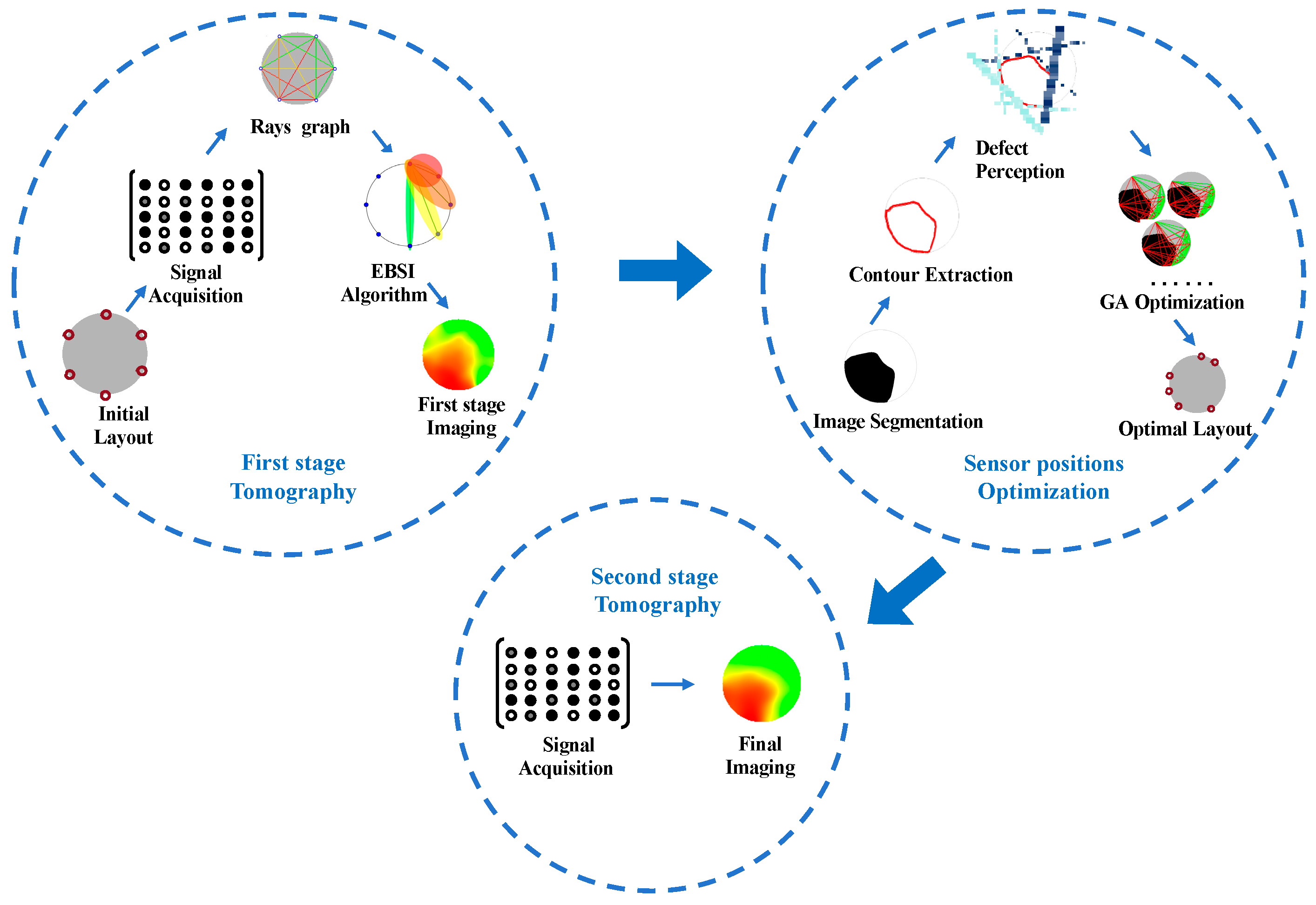
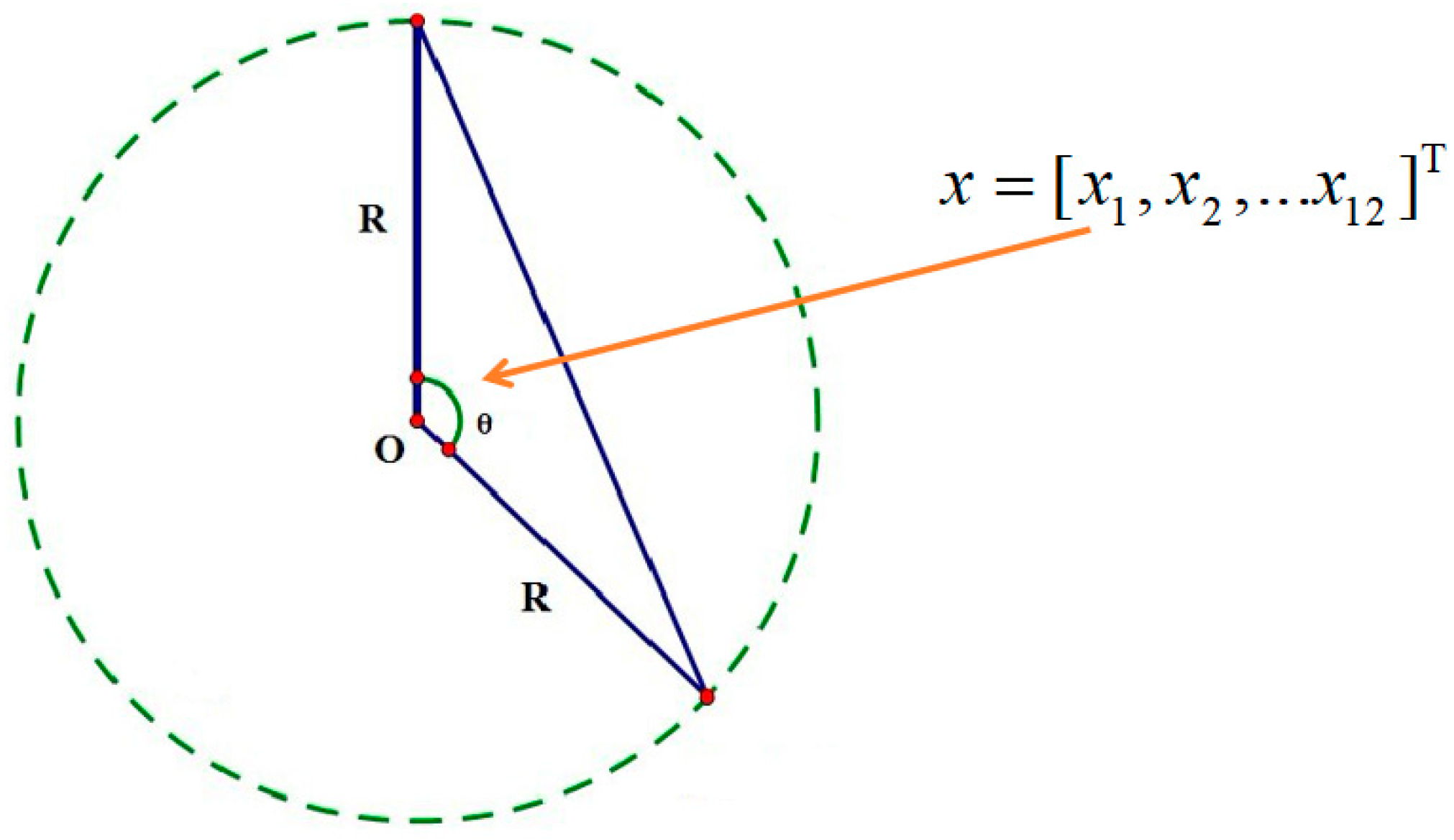
2.3. Optimizing Sensor Positions Based on Defect Distribution Perception

As can be seen from the previous section, both the ray penetration ratio and degree of equidistant distribution of sensors are important factors affecting the tomography results of internal defects in wood. Compared with the signal acquisition strategy using equidistantly distributed sensors, a more optimal planar distribution strategy for stress wave sensors would be to equidistantly set sensors as much as possible on the cross-section of trunks, while ensuring the optimal ray penetration ratio. On this basis, a sensor position’s optimization algorithm using defect distribution perception is proposed in this paper. By using the ray penetration ratio and the degree of equidistant distribution of sensors, the defect distribution pattern can determine the optimal sensor layout. An illustration of this algorithm is shown in Figure 4.

As can be seen in Figure 4, the tomography process is divided into two stages. In the first tomography stage, sensors are equidistantly set, and signal acquisition is conducted in the traditional way, with the EBSI algorithm used as the basic tomographic imaging method to reconstruct the internal defects in the wood. In the second stage, the algorithm enters the stage of sensor position’s optimization. It performs OTSU image segmentation and contour extraction on the first imaging result from the first stage, marks the grid points of the defective area, and counts the area proportion of the reconstructed defects. It also sequentially determines whether each ray has passed through the defective area (the rays are discretized into a set of grid points, and if any grid points have been marked, it is determined that the ray has passed through the defective area) and calculates the ray penetration ratio. Next, sensor position’s optimization is searched using a nonlinear global optimization algorithm, and the tomography process enters the second stage. After the sensors are redistributed according to the optimization strategy, the stress wave signals are collected for the second time, and the image of the internal defects is reconstructed using EBSI again as the final tomography result.

There are many optimization algorithms. Regardless of which optimization algorithm is selected, the key step is to design a reasonable fitness function and optimization conditions [42,43]. The optimization algorithm itself is not studied in this paper; therefore, the classical Genetic Algorithm is selected as the optimization method. In the Genetic Algorithm, there are multiple steps involved, including initializing the population; encoding; and calculating fitness, selection, crossover, and mutation. Considering that the cross-section of the trunks is usually circular, in order to effectively model the distribution status of a set of sensors, as shown in Figure 5, we use the angle to represent the spacing between sensors. Genetic individuals can be represented as follows:

$$x={[x_1,x_2,\dots x_{12}]}^{\mathrm{T}}$$

(1)

where each component x_i is the angle between the straight line formed by the i-th sensor and the center of the circle and the straight line formed by the 1st sensor (located at 12 o’clock) and the center of the circle, with a value range of 0 to $2\pi$. Since individual x is already represented in decomposable vector form, traditional binary encoding is no longer used to encode genetic individuals. The basic idea of this algorithm is to ensure the optimal ray penetration ratio while setting stress wave sensors as equidistantly as possible on the cross-section of trunks. Therefore, the objective function in the Genetic Algorithm can be defined as follows:

$$f(x)=\left|CrossRate-AreaRate\right|\times w_1+(UniRate)\times w_2$$

(2)

where AreaRate is the area proportion of the reconstructed defects obtained using the first-stage tomography result, while CrossRate is the ray penetration ratio, which is calculated in real time based on the status of the genetic individual (the distributed positions of 12 sensors). w₁ and w₂ are two weight coefficients, and because the ray penetration ratio is equally as important as the degree of equidistant distribution of sensors, both weights are set to 0.5. The optimization process is the process of searching the minimum f(x), and UniRate is the degree of the equidistant distribution of 12 sensors corresponding to each genetic individual, which is expressed as follows:

$$UniRate=\frac{\mathrm{Max}-\mathrm{Min}}{\mathrm{Mean}}\times 100\%$$

(3)

where Max is the maximum angle between a pair of adjacent sensors among the 12 sensors, Min is the minimum angle between a pair of adjacent sensors, and Mean is the average angle between each pair of adjacent sensors. The angle between any pair of adjacent sensors can be calculated from the sorted x.

When performing the selection operation, we calculate the fitness function value for each individual, with the fitness function being the reciprocal of the objective function. Each generation selects individuals based on a certain selection probability, retaining individuals with higher fitness for the next generation. When performing the crossover operation, we traverse all individuals pairwise, take one piece of sensor position information x_i from each individual, exchange based on a certain crossover probability, and save the two individuals after crossover. When performing the mutation operation, we traverse all individuals, take one piece of sensor position information x_i, and perform mutation based on a certain mutation probability (changing the new sensor positions by randomly increasing a certain angle). During the process of crossover and mutation, while preventing the optimal search from getting stuck in a local optimal solution, if there are sensors in the new individual with the same position as the old individual, no new individuals are generated to prevent the sensor positions from gathering at the same point. In addition, when the ratio of the average fitness value of the current population to the average fitness value of the previous generation is within [1.0, 1.05] or when the maximum number of iterations is reached, the algorithm terminates.

Finally, the specific process of the stress wave sensor position’s optimization algorithm based on defect distribution perception is proposed. The flowchart is shown in Figure 6.

The specific steps in the flowchart are as follows:

Step 1: Normalize the collected stress wave propagation velocity matrix and visualize it as a ray graph while generating the grid graph for tomography.

Step 2: Use the EBSI algorithm for the first stage of stress wave tomography, and then perform image segmentation. Divide the imaging results into defective areas and healthy areas, and then calculate the area proportion of the reconstructed defects and the ray penetration ratio separately.

Step 3: Initialize the population, randomly generate a certain number of sensor positions as the initial population, calculate the fitness value of each individual in the initial population, and then enter the genetic deduction process.

Step 4: Perform selection, crossover, and mutation operations on the contemporary population, and recalculate the fitness values of each individual in the population.

Step 5: Determine whether the termination condition of the optimization algorithm is met. If not, repeat step 4.

Step 6: Genetic deduction ends, sort the last generation population according to the fitness values, and select the best individual after sorting as the final sensor layout strategy.

Step 7: Reset each sensor location according to the optimized sensor layout strategy, repeat steps 1 and 2, and achieve stress wave tomography in the second stage.

Step 8: Reconstruct and visualize an image of the defects by using the estimated velocity values in the grid points.

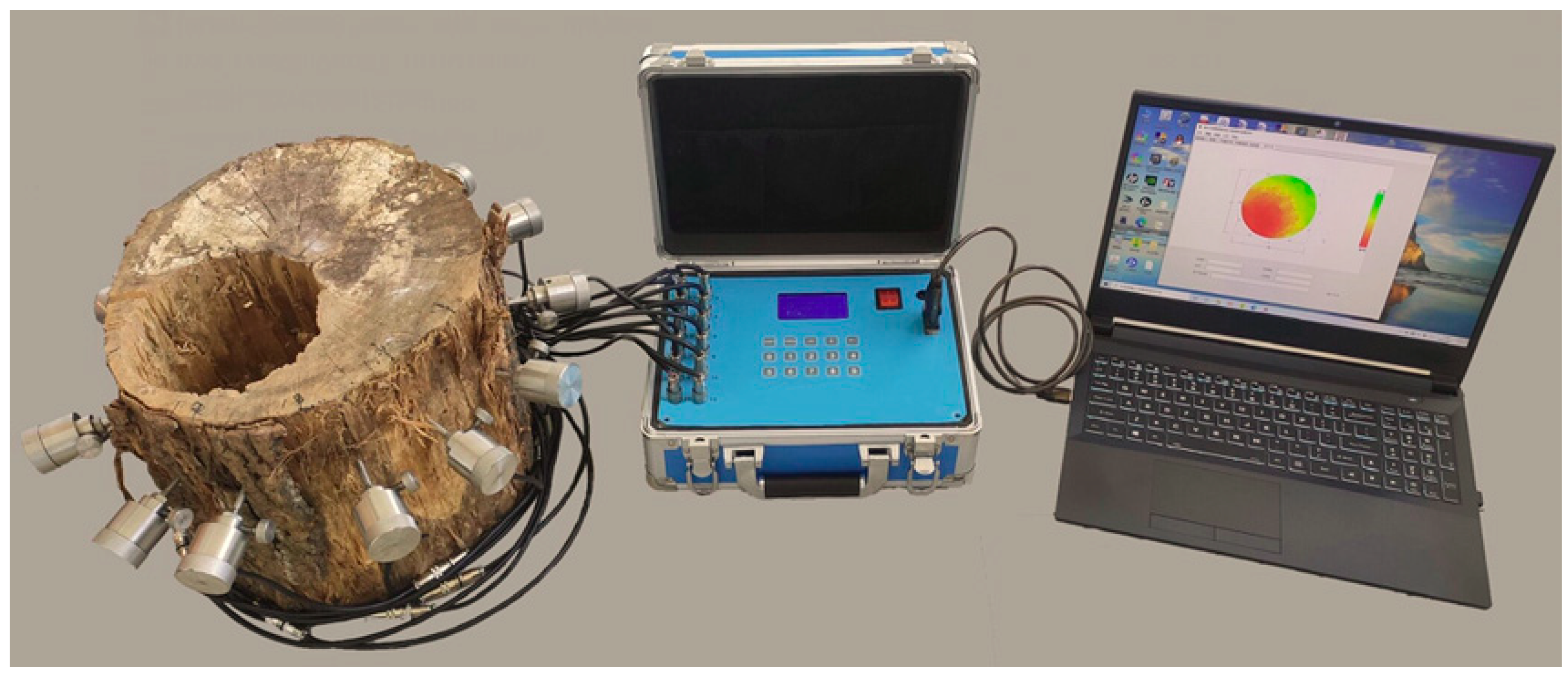
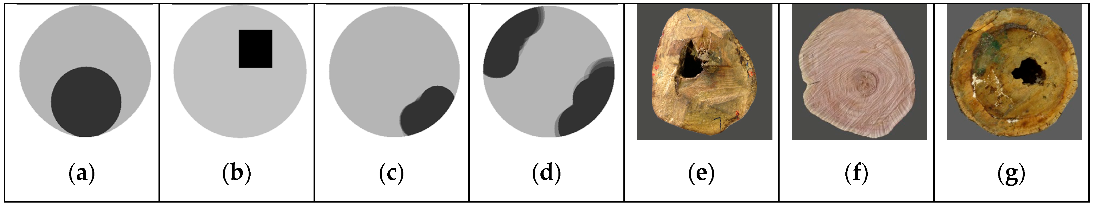
2.4. Signal Acquisition and Experimental Samples

In the experiment, a self-developed stress wave signal acquisition instrument named Wopecker (v2.0, Hangzhou, China) was adopted. The experimental setup is shown in Figure 7. The instrument consists of 12 stress wave sensors, a signal processor unit, software, an electronic hammer, and several data wires. When performing stress wave imaging on hardwood samples, we place 12 piezoelectric-type sensors at certain cross-sections of the tree trunk and knock each sensor in sequence, and the remaining sensors receive the generated stress wave signals. Next, the signal processing unit analyzes the received signal based on digital signal processing technology (short-time energy and double threshold detection are used to estimate the stress wave propagation time), and the corresponding stress wave propagation time matrix is obtained. The signal processing box then transmits the time matrix to the computer (CPU: Intel Core i3 2.10 GHz; RAM: 8 GB) through a USB connection. The distance between any pair of sensors is known, so the complete velocity matrix can be displayed and calculated by the self-developed software (v2.0, Hangzhou, China) as the input data of the proposed method.

In order to comprehensively evaluate the imaging performance of the proposed method, we designed simulated and real samples in the experimental stage. In the simulation experiment, there were four virtual samples, and the size and shape of the defects in each sample were different. The shape and area of the virtual defects were defined manually, and the corresponding ray graph was also defined manually. Figure 8 shows the four virtual defects, including a one-circle pattern, a one-rectangle pattern, a one-edge pattern, and a two-edge pattern. In addition, three hardwood samples were used in the experiment: a Chinaberry tree trunk with holes, a Firmiana tree trunk with knots, and a Pecan tree trunk with holes, as shown in Figure 8.

3. Results and Discussion

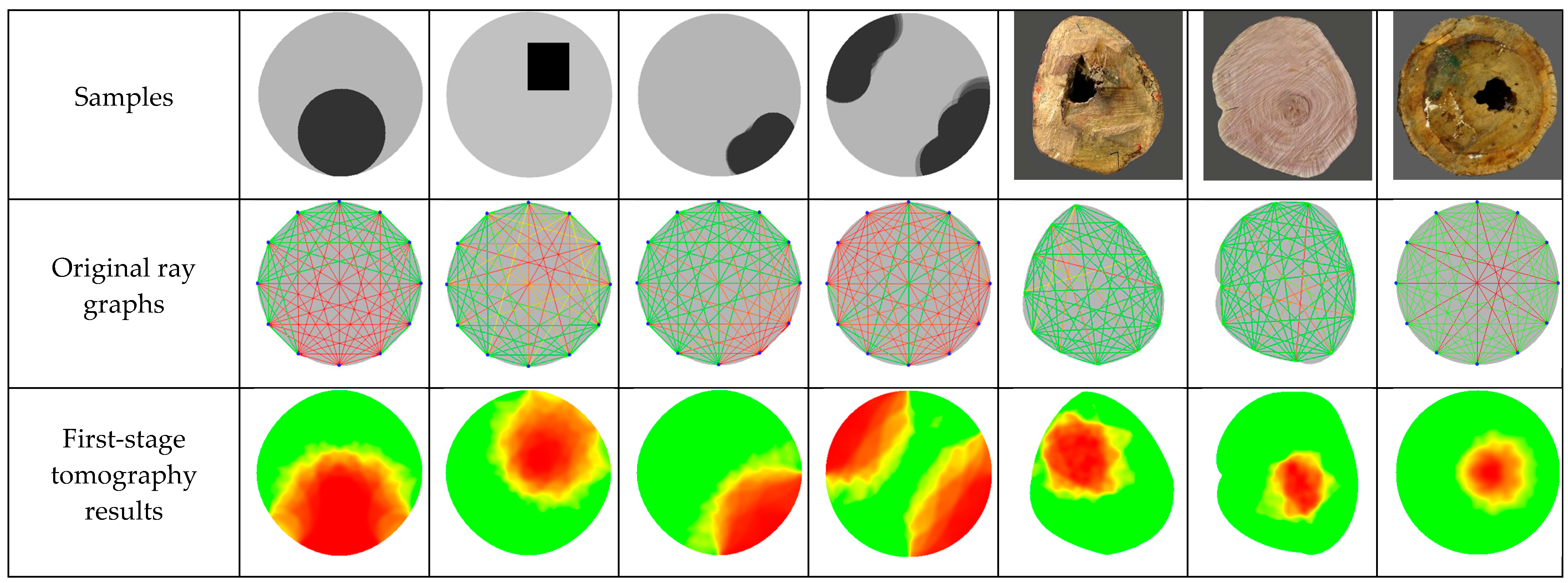
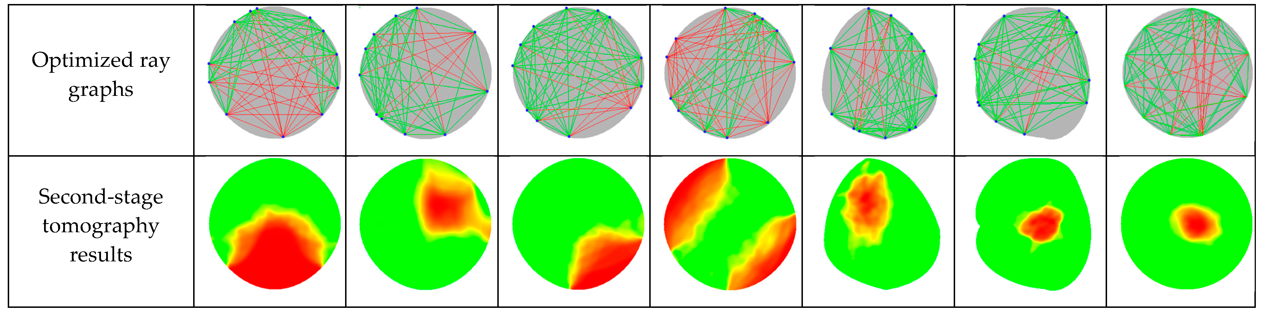
3.1. Tomography Results Based on Proposed Optimization Algorithm for Sensor Positions

In order to obtain high-quality imaging results, we set the number of pixel points in each grid to 1, and the size of the imaging area for defects is 300 × 300 pixels. In addition, for a unified visualization effect, colors from green to red are again used to distinguish stress wave velocity. The faster the estimated velocity within the grid, the greener the color of the grid; the slower the estimated velocity within the grid, the redder the color of the grid.

The initial population size in the proposed algorithm is 200, with a maximum selection probability of 80%, a maximum exchange probability of 25%, and a maximum mutation probability of 5%, and the maximum number of iterations is 50. The defect samples, original ray graphs, first-stage tomography results, optimized ray graphs, and second-stage tomography results are shown in Figure 9.

The comparative tomography experiment results show that the optimized sensor position strategy helps us observe stress wave signals at better angles and also assists in generating stress wave propagation ray graphs that are more conducive to reconstructing the internal defects in hardwood. In addition, compared with the tomography results obtained by equidistantly distributing sensors in the first stage, the tomography results of the proposed method in the second stage are closer to the actual defects in visual perception. For sample 4 in particular, when the sensors were equidistantly distributed, there were too many red rays in the ray graphs, indicating that the ray penetration ratio was not ideal. After optimizing the planar distribution of sensors, the ray penetration ratio tended to be ideal, and the imaging results were significantly improved. For sample 3, the imaging effect did not improve significantly. This is because the ray penetration ratio in the original ray graph of sample 3 was already relatively ideal, and the optimized planar distribution of sensors was not very different from the uniform sensor planar distribution. It can be seen that when the ray penetration ratio in original ray graphs is relatively ideal, the optimization effect is not significant. However, when the ray penetration ratio in original ray graphs is not ideal, the optimization effect is significant.

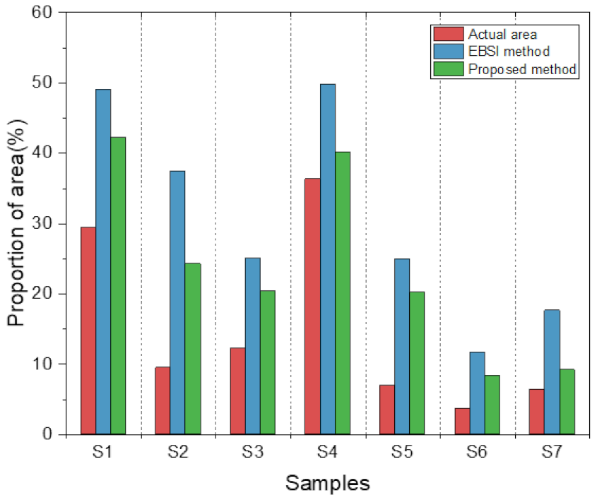
3.2. Area Analysis of Reconstructed Defects

To quantitatively evaluate the sensor position’s optimization algorithm based on the defect distribution perception proposed in this paper, we obtained the reconstructed defective area using the OTSU image segmentation method before and after sensor position’s optimization. The comparison results are presented in Figure 10. It can be seen that all the areas obtained using the proposed method are closer to the areas of the actual area than those derived using the original EBSI method.

In order to compare the area of reconstructed defects before and after sensor position’s optimization with data, the area proportions of the reconstructed defects for all samples in the entire imaging area were calculated, with the comparative analysis results shown in Figure 11. It can be seen that the area ratio of the reconstructed defects is closer to the area ratio of the actual defects after optimizing sensor planar distribution. For sample 2 in particular, the area proportion of reconstructed defects after sensor position’s optimization decreased by nearly 15% compared with the area proportion of reconstructed defects before optimization. Furthermore, the reconstructed defects before optimization adhered to the edges, but after optimizing the sensor positions, adhesion was greatly corrected. An area analysis of the reconstructed defects indicates that, even when using the same image reconstruction algorithm, optimizing the planar distribution of sensors is also a good way for improving the effect of stress wave tomography.

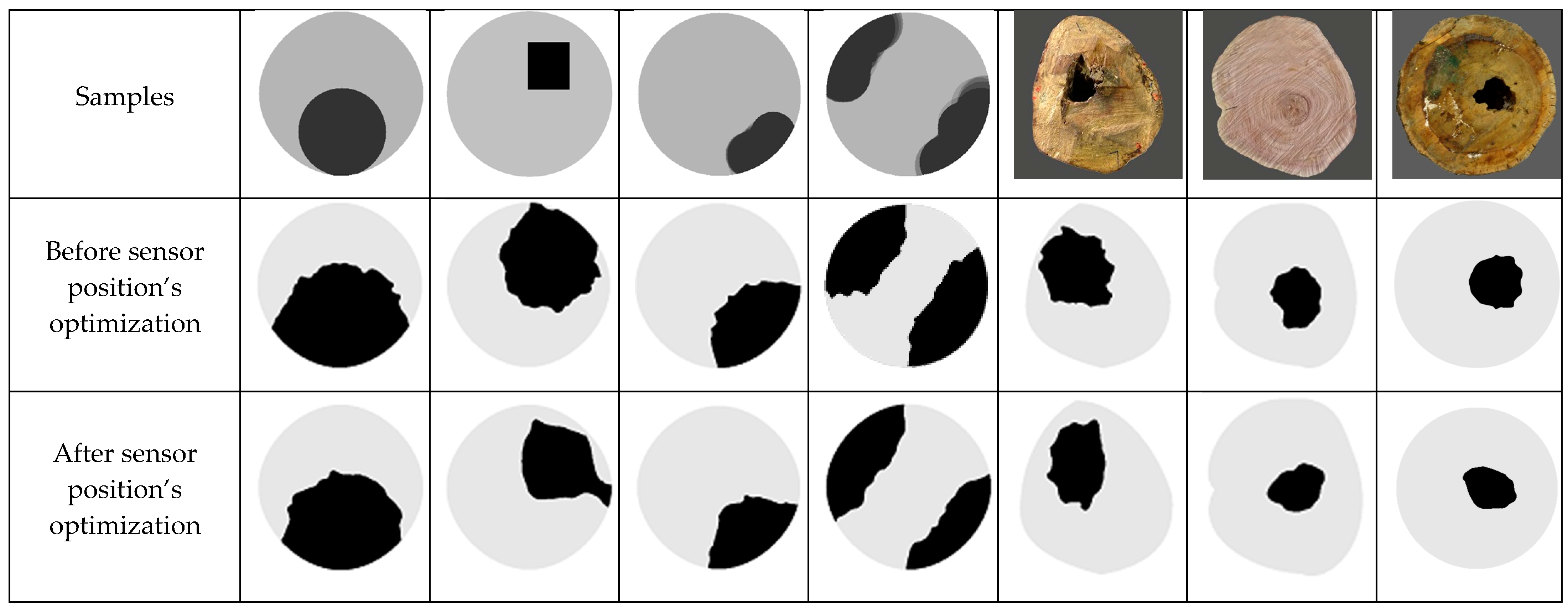
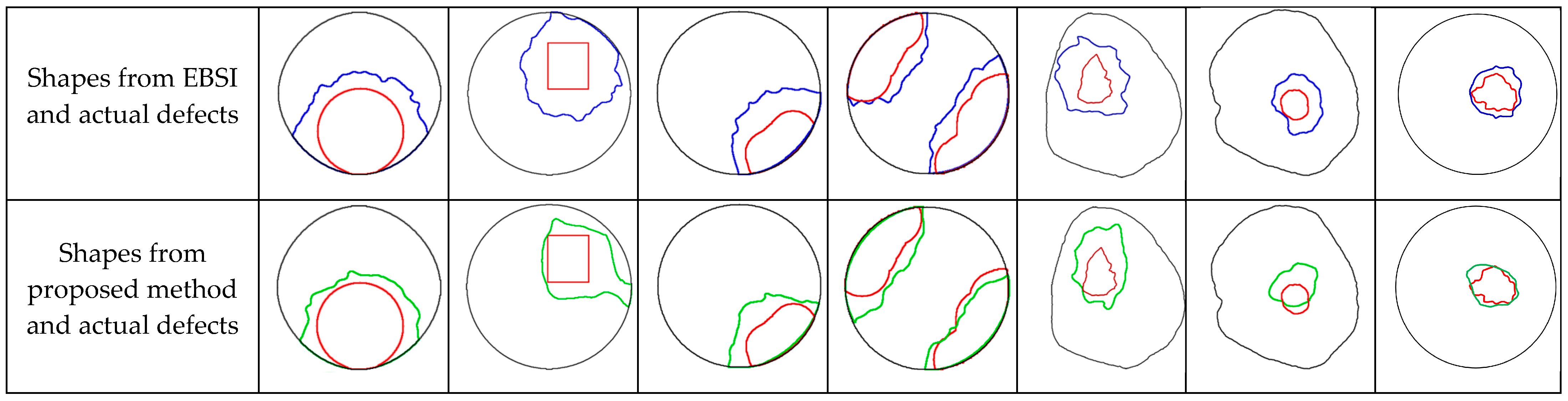
3.3. Shape Analysis of Reconstructed Defects

To analyze the experimental results of stress wave tomography more accurately, we extracted the contours of the reconstructed defects before and after sensor position’s optimization, and we compared them with the actual contours of the internal defects using Photoshop software (v2022). The comparison result is shown in Figure 12.

In Figure 12, the blue line represents the reconstructed defective contour extracted before sensor position’s optimization, the green line represents the reconstructed defective contour extracted after sensor position’s optimization, and the red line represents the actual contour of the defects. These comparative analysis results clearly indicate that, compared with the blue contours, the green contours are closer to the red contours in all samples. This indicates that the proposed algorithm perceived the distribution pattern of the defects through the ray penetration ratio and the degree of equidistant distribution of sensors, and it optimized the planar distribution of sensors through the Genetic Algorithm to improve imaging accuracy by adjusting the observation angles of the stress wave signals.

To quantitatively and more accurately evaluate the quality of our method, we evaluated the overlap degree between the shape of the reconstructed defects and the shape of the actual defects based on the accuracy, precision, and recall of the visualized confused matrix [36].

As shown in Figure 13, TP represents the region that is correctly estimated as internal wood defects. FN represents the region that is incorrectly estimated as sound wood. FP represents the region that is incorrectly estimated as internal wood defects. TN represents the region that is correctly estimated as sound wood. Therefore, the confusion matrix can indicate the overlap degree of two shapes. Quantitative indicators such as accuracy, precision, and recall are calculated as follows:

$$Accuracy=\frac{TP+TN}{TP+TN+FP+FN}, Precision=\frac{TP}{TP+FP}, Recall=\frac{TP}{TP+FN}$$

(4)

The accuracy, precision, and recall of the tomographic imaging algorithm before and after optimizing sensor positions are shown in Figure 14. In terms of recall, the proposed method did not achieve a recall of 80% for sample 6, because the reconstructed defective contour did not fully cover the actual defective contour. Although the traditional EBSI method achieved a recall of 100% for sample 6, it severely overestimated the area and shape of the defects. For other samples, both algorithms had recall rates close to 100%. This result represents that the two methods can effectively locate the position of defects inside hardwood. In terms of accuracy, for all samples, sensor position’s optimization had better tomography results than the original EBSI method. For sample 6 in particular, the proposed method achieved better accuracy than the EBSI method in the case of limited recall performance. This indicates that the contour obtained using the proposed method had a better overlap with the actual contour. The average accuracy of the proposed method was 90.3%, while the average accuracy of the EBSI method was only 84.1%. In terms of precision, for all samples, the proposed method had better tomography results than the original EBSI method again, with an average accuracy improvement of 11.7%. This result indicates that, although the equidistant planar distribution of sensors is already a good data acquisition strategy, the sensor position’s optimization method proposed in this paper further improves the accuracy and precision of stress wave tomography.

4. Conclusions

In this study, a novel sensor position’s optimization method for the stress wave tomography of internal hardwood defects was proposed. In order to evaluate the imaging performance after the proposed sensor position’s optimization method, seven defect samples with different sizes and positions were tested, and the area and shape of the tomography results were quantitatively analyzed. The experimental results support the following conclusions:

(1)

Different from traditional stress wave tomography methods that focus on designing image reconstruction algorithms to improve imaging accuracy, the optimized sensor position strategy proposed in this paper also improves imaging accuracy. After optimizing the planar distribution of sensors, the area of reconstructed defects is closer to the area of actual defects, and the contour of reconstructed defects is also closer to the contour of actual defects.

(2)

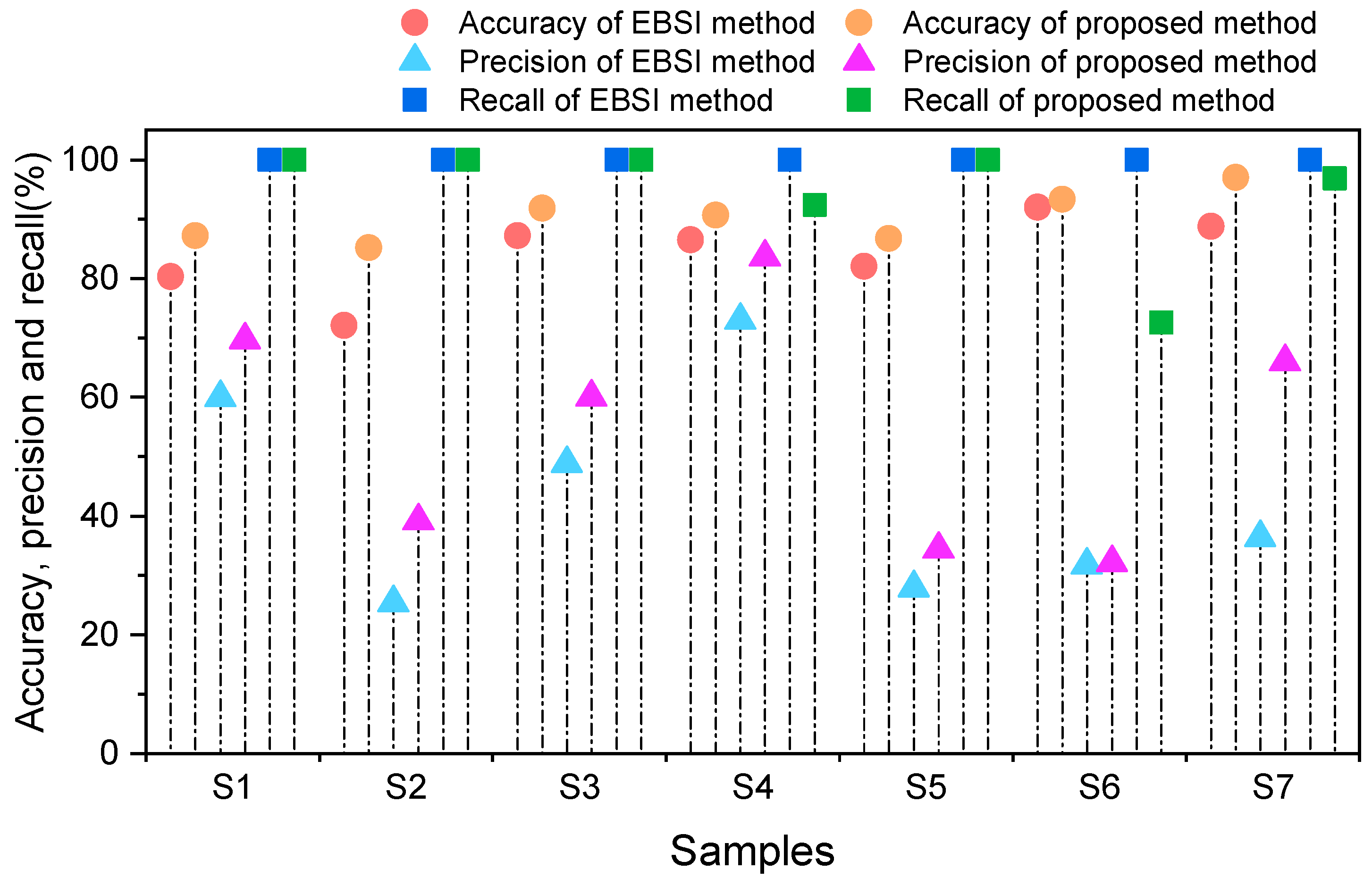
The proposed algorithm perceived the space distribution pattern of defects through the ray penetration ratio defined in this paper, improved the quality of the tomography algorithm input data through the optimization of sensor positions, and helped obtain better tomography results. After optimizing the planar distribution of sensors, the average accuracy of the EBSI method increased by 6.2% compared with the original EBSI method, while the average accuracy increased by 11.7%.

(3)

The traditional clock distribution of 12 sensors for data acquisition is a simple and usable strategy that can be used as a universal sensor layout for the stress wave tomography of internal hardwood defects. However, in situations where the ray penetration ratio is not ideal or when there is a need to achieve high-quality defect reconstruction, the sensor position’s optimization method proposed in this paper can effectively improve the quality of stress wave tomography.

In general, the proposed method can enable the traditional EBSI method to produce a more accurate reconstructed image of internal hardwood defects after optimizing the sensor positions. The ray penetration ratio and the degree of equidistant distribution of sensors are used to establish the fitness function and optimal conditions. These two proposed indicators play a key role in the proposed algorithm. Perhaps there are other potential indicators that can be used, such as the location of defects, the shape of defects, and the contrast of ray color in the ray graph. In addition, the sensor position’s optimization algorithm can be further improved in future work. On the other hand, we used hardwood samples to test the performance of the algorithm in this study. Stress waves propagate slower in softwood than in hardwood, resulting in poor ray color contrast in ray graphs, which is not conducive to the subsequent tomography algorithm. This is the current deficiency of stress wave technology, so it is necessary to study how to enhance stress wave signals to develop this technology.

References

1. Kobza, M.; Ostrovsk, R.; Adamčíková, K.; Pastirčáková, K. Stability of trees infected by wood decay fungi estimated by acoustic tomography: A field survey. Trees 2021, 36, 103–112. [Google Scholar] [CrossRef]
2. Madhoushi, M.; Ebrahimi, S.; Omidvar, A. Structural health assessment of a historical building by using in situ stress wave ndt: A case study in iran. Cerne 2021, 27, e-102535. [Google Scholar] [CrossRef]
3. Radwan, M.; Thiel, D.; Espinosa, H. Single-sided microwave near-field scanning of pine wood lumber for defect detection. Forests 2021, 12, 1486. [Google Scholar] [CrossRef]
4. Cascón, I.; Sarasua, J.; Tena, M.; Uria, A. Development of an acoustic method for wood disease assessment. Comput. Electron. Agric. 2021, 186, 106195. [Google Scholar] [CrossRef]
5. Tomazello, M.; Brazolin, S.; Chagas, M.P.; Oliveira, J.T.S.; Ballarin, A.W.; Benjamin, C.A. Application of x-ray technique in nondestructive evaluation of eucalypt wood. Maderas-Cienciay Tecnol. 2008, 10, 139–150. [Google Scholar] [CrossRef]
6. Ken, W.; Yukie, S.; Stavros, A.; Satoshi, S. Non-destructive measurement of moisture distribution in wood during drying using digital x-ray microscopy. Drying Technol. 2008, 26, 590–595. [Google Scholar]
7. Rinn, F.; Schweingruber, F.; Schär, E. RESISTOGRAPH and X-ray Density Charts of Wood. Comparative Evaluation of Drill Resistance Profiles and X-ray Density Charts of Different Wood Species. Holzforschung 1996, 50, 303–311. [Google Scholar] [CrossRef]
8. Tannert, T.; Anthony, R.; Kasal, B.; Kloiber, M.; Piazza, M.; Riggio, M.; Rinn, F.; Widmann, R. In Situ Assessment of Structural Timber Using Semi-Destructive Techniques. Mater. Struct. 2013, 47, 767–785. [Google Scholar] [CrossRef]
9. Dackermann, U.; Crews, K.; Kasal, B.; Li, J.; Riggio, M.; Rinn, F.; Tannert, T. In situ assessment of structural timber using stress-wave measurements. Mater. Struct. 2014, 47, 787–803. [Google Scholar] [CrossRef]
10. Yamasaki, M.; Tsuzuki, C.; Sasaki, Y.; Onishi, Y. Influence of moisture content on estimating young’s modulus of full-scale timber using stress wave velocity. J. Wood Sci. 2017, 63, 225–235. [Google Scholar] [CrossRef]
11. Yang, Z.; Jiang, Z.; Hse, C.; Liu, R. Assessing the impact of wood decay fungi on the modulus of elasticity of slash pine (pinus elliottii) by stress wave non-destructive testing. Int. Biodeterior. Biodegrad. 2017, 117, 123–127. [Google Scholar] [CrossRef]
12. Garcia, R.; Carvalho, A.; Matos, J.; Santos, W.; Silva, R. Nondestructive evaluation of heat-treated eucalyptus grandis, hill ex maiden wood using stress wave method. Wood Sci. Technol. 2012, 46, 41–52. [Google Scholar] [CrossRef]
13. Wessels, C.; Malan, F.; Rypstra, T. A review of measurement methods used on standing trees for the prediction of some mechanical properties of timber. Eur. J. For. Res. 2011, 130, 881–893. [Google Scholar] [CrossRef]
14. Legg, M.; Bradley, S. Measurement of stiffness of standing trees and felled logs using acoustics: A review. J. Acoust. Soc. Am. 2017, 139, 588–604. [Google Scholar] [CrossRef] [PubMed]
15. Wang, X.; Allison, R. Decay detection in red oak trees using a combination of visual inspection, acoustic testing, and resistance microdrilling. Arboric. Urban. For. 2008, 34, 1–4. [Google Scholar] [CrossRef]
16. Ross, R.; Brashaw, B.; Pellerin, R. Nondestructive evaluation of wood. For. Prod. J. 1998, 48, 14–19. [Google Scholar]
17. Johnstone, D.; Moore, G.; Tausz, M.; Nicolas, M. The measurement of wood decay in landscape trees. Arboric. Urban. For. 2010, 36, 121–127. [Google Scholar] [CrossRef]
18. Mattheck, C.; Bethge, K. Detection of decay in trees with the Metriguard Stress Wave Timer. J. Arboric. 1993, 19, 374–378. [Google Scholar] [CrossRef]
19. Rabe, C.; Ferner, D.; Fink, S.; Schwarze, F. Detection of decay in trees with stress waves and interpretation of acoustic tomograms. Arboric. Assoc. J. 2004, 28, 3–19. [Google Scholar] [CrossRef]
20. Godio, A.; Sambuelli, L.; Socco, L. Application and comparison of three tomographic techniques for detection of decay in trees. J. Arboric. 2003, 28, 3–19. [Google Scholar]
21. Deflorio, G.; Fink, S.; Schwarze, F. Detection of incipient decay in tree stems with sonic tomography after wounding and fungal inoculation. Wood Sci. Technol. 2008, 42, 117–132. [Google Scholar] [CrossRef]
22. Li, L.; Wang, X.; Wang, L.; Allison, R. Acoustic tomography in relation to 2d ultrasonic velocity and hardness mappings. Wood Sci. Technol. 2012, 46, 551–561. [Google Scholar] [CrossRef]
23. Liang, S.; Fu, F. Effect of sensor number and distribution on accuracy rate of wood defect detection with stress wave tomography. Wood Res. 2014, 59, 521–531. [Google Scholar]
24. Lin, C.; Chang, T.; Juan, M.; Lin, T.; Tseng, C.; Wang, Y. Stress wave tomography for the quantification of artificial hole detection in camphor trees (cinnamomum camphora). Taiwan. J. For. Sci. 2011, 26, 17–32. [Google Scholar]
25. Gejdoš, M.; Michajlová, K.; Gretsch, D. The use of the acoustic tomograph and digital image analysis in the qualitative assessment of harvested timber—case study. Cent. Eur. For. J. 2023, 69, 106–111. [Google Scholar] [CrossRef]
26. Qiu, Q.; Qin, R.; Lam, J.; Tang, A.; Leung, M.; Lau, D. An innovative tomographic technique integrated with acoustic-laser approach for detecting defects in tree trunk. Comput. Electron. Agric. 2019, 156, 129–137. [Google Scholar] [CrossRef]
27. Arciniegas, A.; Brancheriau, L.; Lasaygues, P. Tomography in standing trees: Revisiting the determination of acoustic wave velocity. Ann. For. Sci. 2015, 72, 685–691. [Google Scholar] [CrossRef]
28. Zeng, B.; Li, X.; Mao, Z. Correlation inversion detection algorithm and imaging simulation of wood defects focused by stress signal based on symlets wavelet. J. Phys. Conf. Ser. 2020, 1651, 012085. [Google Scholar] [CrossRef]
29. Wei, X.; Xu, S.; Sun, L.; Tian, C.; Du, C. Propagation velocity model and two-dimensional defect imaging of stress wave in larch (larix gmelinii) wood. BioResources 2021, 4, 6799. [Google Scholar] [CrossRef]
30. Zhan, H.; Jiao, Z.; Li, G. Velocity Error Correction Based Tomographic Imaging for Stress Wave Nondestructive Evaluation of Wood. Bioresources 2018, 13, 2530–2545. [Google Scholar]
31. Wang, X.; Wiedenbeck, J.; Liang, S. Acoustic tomography for decay detection in black cherry trees. Wood Fiber Sci. 2009, 41, 127–137. [Google Scholar]
32. Wang, X. Acoustic measurements on trees and logs: A review and analysis. Wood Fiber Sci. 2013, 47, 965–975. [Google Scholar] [CrossRef]
33. Yue, X.; Wang, L.; Wacker, J. Electric resistance tomography and stress wave tomography for decay detection in trees-a comparison study. PeerJ 2019, 7, e6444. [Google Scholar] [CrossRef]
34. Giryes, R.; Eldar, Y.; Bronstein, A.; Sapiro, G. Tradeoffs between convergence speed and reconstruction accuracy in inverse problems. IEEE Trans. Signal Process 2018, 66, 1676–1690. [Google Scholar] [CrossRef]
35. Zeng, L.; Lin, J.; Huang, L. A modified lamb wave time-reversal method for health monitoring of composite structures. Sensors 2017, 17, 955. [Google Scholar] [CrossRef]
36. Hettler, J.; Tabatabaeipour, M.; Delrue, S.; Van, D. Linear and nonlinear guided wave imaging of impact damage in cfrp using a probabilistic approach. Materials 2016, 9, 901. [Google Scholar] [CrossRef]
37. Du, X.; Li, S.; Li, G.; Feng, H.; Chen, S. Stress Wave Tomography of Wood Internal Defects using Ellipse-Based Spatial Interpolation and Velocity Compensation. Bioresources 2015, 10, 3948–3962. [Google Scholar] [CrossRef]
38. Qin, R.; Qiu, Q.; Lam, J.; Tang, A.; Leung, M.; Lau, D. Health assessment of tree trunk by using acoustic-laser technique and sonic tomography. Wood Sci. Technol. 2018, 52, 1113–1132. [Google Scholar] [CrossRef]
39. Strobel, A.; Renato, J.; Carvalho, G.; Antonio, M.; Goncalves, R. Quantitative image analysis of acoustic tomography in woods. Eur. J. Wood Wood Prod. 2018, 76, 1379–1389. [Google Scholar] [CrossRef]
40. Du, X.; Li, J.; Feng, H.; Chen, S. Image reconstruction of internal defects in wood based on segmented propagation rays of stress waves. Appl. Sci. 2018, 8, 1778. [Google Scholar] [CrossRef]
41. Wang, L.; Xu, H.; Yan, Z. Effects of sensor quantity and planar distribution on testing results of log defects based on stress wave. Sci. Silvae Sin. 2008, 44, 115–121. [Google Scholar]
42. Deb, K.; Jain, H. An Evolutionary Many-Objective Optimization Algorithm Using Reference-Point-Based Nondominated Sorting Approach, Part I: Solving Problems With Box Constraints. IEEE Trans. Evol. Comput. 2014, 18, 577–601. [Google Scholar] [CrossRef]
43. He, S.; Wu, Q.; Saunders, J. Group search optimizer: An optimization algorithm inspired by animal searching behavior. IEEE Trans. Evol. Comput. 2009, 13, 973–990. [Google Scholar] [CrossRef]
Figure 1. (a) Ray graph; (b) grids of imaging area; (c) EBSI diagram.
Forests 15 00465 g001
Figure 2. Visualization of the relationship between ray penetration ratio and area proportion of reconstructed defects.
Forests 15 00465 g002
Figure 3. Tomographic imaging results when sensors are extremely unequally spaced.
Forests 15 00465 g003
Figure 4. Illustration of stress wave sensor position’s optimization algorithm based on defect distribution perception.
Forests 15 00465 g004
Figure 5. Illustration of a genetic individual represented by the angle.
Forests 15 00465 g005
Figure 6. Flowchart of proposed method.
Forests 15 00465 g006
Figure 7. The experimental setup.
Forests 15 00465 g007
Figure 8. Simulated and real samples: (a) one-circle pattern; (b) one-rectangle pattern; (c) one-edge pattern; (d) two-edge pattern; (e) tree trunk with holes; (f) tree trunk with knots; (g) tree trunk with holes.
Forests 15 00465 g008
Figure 9. Comparison of tomography results before and after sensor position’s optimization.
Forests 15 00465 g009aForests 15 00465 g009b
Figure 10. Comparison of reconstructed defective areas before and after sensor position’s optimization.
Forests 15 00465 g010
Figure 11. Comparison of area proportion of reconstructed defects.
Forests 15 00465 g011
Figure 12. Comparison of the shape of reconstructed defects.
Forests 15 00465 g012aForests 15 00465 g012b
Figure 13. Diagram of confusion matrix.
Forests 15 00465 g013
Figure 14. Comparison of accuracy, precision, and recall.
Forests 15 00465 g014
Disclaimer/Publisher’s Note: The statements, opinions and data contained in all publications are solely those of the individual author(s) and contributor(s) and not of MDPI and/or the editor(s). MDPI and/or the editor(s) disclaim responsibility for any injury to people or property resulting from any ideas, methods, instructions or products referred to in the content.