Abstract
Accurate classification of forest tree species holds great significance in the context of forest biodiversity assessment and the management of forest resources. In this study, we utilized Sentinel-2 time series data with high temporal and spatial resolution for tree species classification. To address potential classification errors stemming from spectral differences due to tree age variations, we implemented the Continuous Change Detection and Classification (CCDC) algorithm to estimate tree ages, which were integrated as additional features into our classification models. Four different combinations of classification features were created for both the random forest (RF) algorithm and extreme gradient boosting (XGB) algorithm: spectral band (Spec), spectral band combined with tree age feature (SpecAge), spectral band combined with spectral index (SpecVI), and spectral band combined with spectral index and tree age feature (SpecVIAge). The results demonstrated that the XGB-based models outperformed the RF-based ones, with the SpecVIAge model achieving the highest accuracy at 78.8%. The incorporation of tree age as a classification feature led to an improvement in accuracy by 2% to 3%. The improvement effect on classification accuracy varies across tree species, due to the varying uniformity of tree age among different tree species. These results also showed it is feasible to accurately map regional tree species based on a time-series multi-feature tree species classification model which takes into account tree age.
1. Introduction
Accurate and comprehensive mapping of tree species serves as the foundation for forest resource management and forestry development. It is indispensable for biodiversity conservation and monitoring of forest carbon stocks [1,2]. Simultaneously, considering the profound sensitivity of forest ecosystems to climate change, tree species information becomes crucial for assessing the potential ecological impact of future climatic shifts on forest ecosystems [3]. Historically, conventional fieldwork was the primary approach. However, its application was constrained by survey costs and accessibility issues. This limitation made it challenging to provide a detailed composition of tree species across extensive areas [4,5,6].
Remote sensing technology offers an efficient means of gathering species information, providing valuable insights into their spatial distribution. Additionally, it enables the collection of repeatable data observations across vast geographical areas, effectively meeting the increasing demand for data [7,8,9]. The mapping of forest species using remote sensing data has gained significant attention in recent decades [10,11]. Typically, very high-resolution data (VHR) such as Worldview and GF-2 have been employed for detailed tree species mapping [12,13]. Nevertheless, due to their high acquisition costs and limited availability, VHR are primarily suitable for tree species classification tasks in smaller regions [10,14]. In contrast, medium-resolution multispectral data are typically used for larger geographical areas with complex ecological settings, such as Landsat images and Sentinel-2 images, due to their continuity, affordability, and accessibility features [15,16,17]. A recurring theme in these studies is that classification based on multi-temporal remote sensing data often outperforms single-image-based classification, especially when different vegetation phenology stages are captured [16,18,19,20,21]. Markus I. et al. [19] demonstrated that multi-temporal classification models produce superior results compared to single images, especially when acquired based on phenological stages, showcasing the best classification effectiveness. Similarly, Joseph J. et al. [21] also found that aligning the collection date of remote sensing images with the phenological stage of tree species in the study area can improve discrimination of the dry deciduous forest class from the rainforest class. This is because different tree species display unique physiological and biochemical characteristics at multiple phenological stages. The spectral separability between tree species is enhanced in different phenological stages, which can be utilized for more accurate mapping of tree species [22].
However, the classification based on multi-temporal remote sensing data also exposes a notable limitation: the continuous evolution of vegetation phenology may lead to incomplete capture of phenological information due to the sparsity of the data [18]. To overcome the limitation, the tree species classification method based on time series remote sensing data has gained increasing attention [23,24]. This approach utilizes denser data to capture continuous and complete phenological changes, resulting in superior classification results compared to methods relying solely on multi-temporal or single images [25,26]. For example, in the tree species mapping task within complex mixed forests, Grabska E. et al. [16] demonstrated that the main reason for the 5–10% improvement in classification accuracy was the use of time series data. Notably, the launch of the Sentinel-2 satellites in 2015 and 2017 marked a significant advancement in the spatial-temporal resolution of multispectral remote sensing data. The 5-day revisit interval and a spatial resolution of 10–20 m have substantially enhanced land cover identification [16,18,19,23]. Therefore, the use of Sentinel-2 data for constructing time series can provide more detailed surface observation data, potentially resulting in improved classification accuracy [23]. Hemmerling J. et al. [27] utilized Sentinel-2 time series data combined with texture features and environmental data to produce a high-precision map of 17 temperate tree species, which demonstrated the significant contribution of time series images for tree species classification. Huang Z. et al. [28] extracted the spectrum–temporal features of the Sentinel-2-data-based deep learning approach and applied them to the classification of tree species in plantation. The final results confirmed that the time series data could effectively utilize phenological information to improve the classification accuracy of tree species.
A significant challenge in tree classification based on remote sensing data is the spectral variability exhibited by the same tree species. This variability often arises from the morphological and growth adaptations of tree species to their environments, leading to spectral confusion and affecting classification accuracy [29,30,31]. To address this variability, topographic and climatic data are commonly used as auxiliary information to enhance the classification effect [30,31,32]. For instance, Hermosilla T. et al. [33] highlighted that incorporating topographic factors as auxiliary classification data can significantly enhance classification accuracy. He emphasized the effectiveness of topographic features in mitigating forest spectral variability. However, one often-overlooked factor is the impact of tree age on spectral characteristics. The same tree species at different ages can exhibit significant spectral variability due to variations in their form and growth. Spectral differences within the same tree species at different ages contribute to classification errors. Hemmerling J. et al. [27] speculated that dividing the reference samples of the same tree species into subclasses according to tree age might reduce the intra-class variability of the tree species. This viewpoint was supported by Grabska E. et al. [16], who believed that the effect of tree age on the spectral reflectance of forests would often lead to species differences in reflectance, and the classification errors caused by such differences would not be eliminated even with additional environmental variables such as soil and terrain data. Therefore, the spectral variability within tree species caused by tree age, which has negative effects on forest classification accuracy, must be considered. The confirmation of whether tree age, as a classification feature, can eliminate the classification error of forest tree species remains a question.
Our study aimed to achieve the precise classification of dominant tree species in the study area by utilizing Sentinel-2 time series data along with the tree age feature derived from extensive time series Landsat images. The random forest (RF) and extreme gradient boosting (XGB) algorithms, acknowledged for their exceptional performance, were used to construct classification models based on various feature combinations to verify the effectiveness of tree ages as a classification feature.
2. Study Area and Data
2.1. Study Area
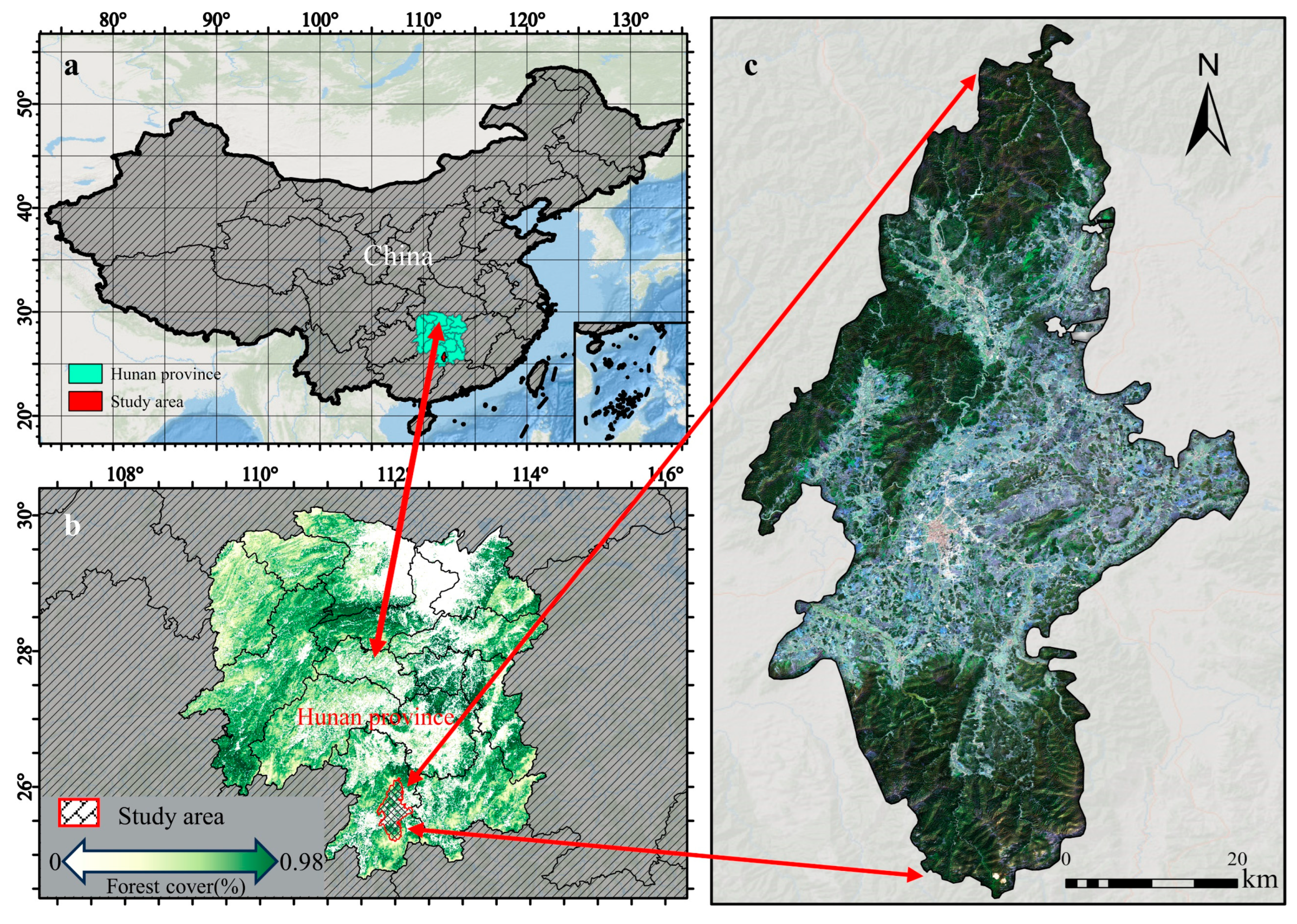
Our study area is situated in Ningyuan County, Hunan Province, China, encompassing an area of more than 2500 km2 (Figure 1). The region experiences a subtropical monsoon climate characterized by abundant rainfall and well-developed water systems. Surrounded by mountains on all sides, the highest elevation in the research area reaches 1959.2 m, while the lowest is at 165 m. The mountainous area constitutes 63% of the total county area. The forest ecosystem, covering more than 60% of the study area, is predominantly composed of evergreen forests, encompassing a wide range of tree ages. The dominant tree species in the study area include cypress (Cupressus), horsetail pine (Pinus massoniana), wetland pine (Pinus elliotii), fir (Cunninghamia Lanceolata (Lamb.) Hook), and eucalyptus (Eucalyptus), which account for over 90% of the forested area. They are also the representative dominant tree species in the southern regions of China. Less common species are oak (Quercus), camphor (Cinnamomum camphora), etc. The main growing season is April to September, starting later (and ending earlier) at higher elevation zones, peaking in usually wet and warm summers.

Figure 1.
The study area of Ningyuan County in southern Hunan Province, China. (a) represents the location of the study area in China; (b) represents the forest cover of the study area; (c) represents the Sentinel-2 imagery of the study area.
2.2. Data
2.2.1. Sentinel-2 Data
In this study, Sentinel-2 images with cloud cover less than 50% in the research area from 1 January 2020 to 31 December 2020 were collected using Google Earth Engine (GEE). The seamless and cloud-free data of each month was performed by image mosaicking. The temporal distribution of the final 18 gap-free images obtained was as follows: two images per month in January, March, November, and December, three images in September, and one image per month in the remaining months. Subsequently, the QA band was used in GEE to mask clouds and cloud shadows for each image to improve data quality. Finally, the 20 m bands were resampled using a nearest-neighbor technique to match the resolution of the 10 m bands.
The specific spectral bands utilized for classification encompassed B2 (blue), B3 (green), B4 (red), B5–B7 (red edge), B8 (near-infrared), and B11–B12 (shortwave-infrared). Additionally, eight commonly used spectral indices essential for current tree species classification research were calculated. Please refer to Table 1 for the calculation methods of these vegetation indices.

Table 1.
Calculation formulas for the spectral index feature variables.
2.2.2. Landsat Data
Given the extended lifespan of forests spanning over a hundred years, considering the timespan of remote sensing data becomes crucial when employing change detection methods to estimate forest age. The GEE platform was utilized to retrieve all available Landsat images within our research area from 1986 (the earliest Landsat images accessible on the GEE platform) to 2020, including images collected by the Thematic Mapper (TM), Enhanced Thematic Mapper Plus (ETM+), and Operational Land Imager (OLI) sensors. Subsequently, after mosaicking the images on a monthly basis, the images corresponding to the same season each year were used to minimize the potential for misinterpreting land cover changes due to phenological or solar position variations. To enhance data quality, the QA band was also used to remove clouds and cloud shadows from the acquired Landsat data. In addition, spectral indices, including NDVI and NBR [41] were calculated to facilitate forest disturbance detection [42]. This is because, for healthy and lush forests, NDVI and NBR generally exhibit higher values and are more sensitive to forest disturbance and restoration [41,43]. These extensive time series Landsat images and spectral indices will serve as valuable data sources for determining the age of the forest in the study area using change detection algorithms. Please refer to Table 2 for the calculation methods of these vegetation indices.
Table 2.
Calculation formulas for the spectral indices used for change detection.
2.2.3. Reference Data
The forest tree species sample data utilized in this study were derived from the 2020 forest resources survey data of Hunan Province. The survey data provide information for tree stand units, such as tree species, basal area, and volume. The objects of classification in this study are five dominant tree species in the research area: cypress, horsetail pine, wetland pine, fir, and eucalyptus. To ensure the spatial correspondence between field data and imagery, we conducted field surveys in the study area, used the ‘OvitalMap’ software to record the precise GPS coordinates of the sample points, and ensured that the remote sensing imagery and sample data shared a consistent coordinate system. Since the spatial resolution of the forest cover data obtained for 2020 is 30 m [44], to ensure the subsequent assessment of forest coverage within the samples, we excluded sample data with an area less than 30 m × 30 m. Tree stand units meeting any of the following criteria were excluded: tree cover less than 50%, trees affected by recent disturbance events such as drought or insect outbreaks, trees with obviously incorrect attributions, and those with geolocation errors [27]. Additionally, samples of other non-wooded lands within the study area were selected, based on 2020 Google Earth imagery. In total, 2328 high-quality sample units were selected within the study area, and the categories and numbers of these sample units are detailed in Table 3. Subsequently, the sample data were randomly split into a training set and a validation set at a ratio of 7:3 for the training and prediction of the classification model.
Table 3.
Category and number of sample units.
3. Methods
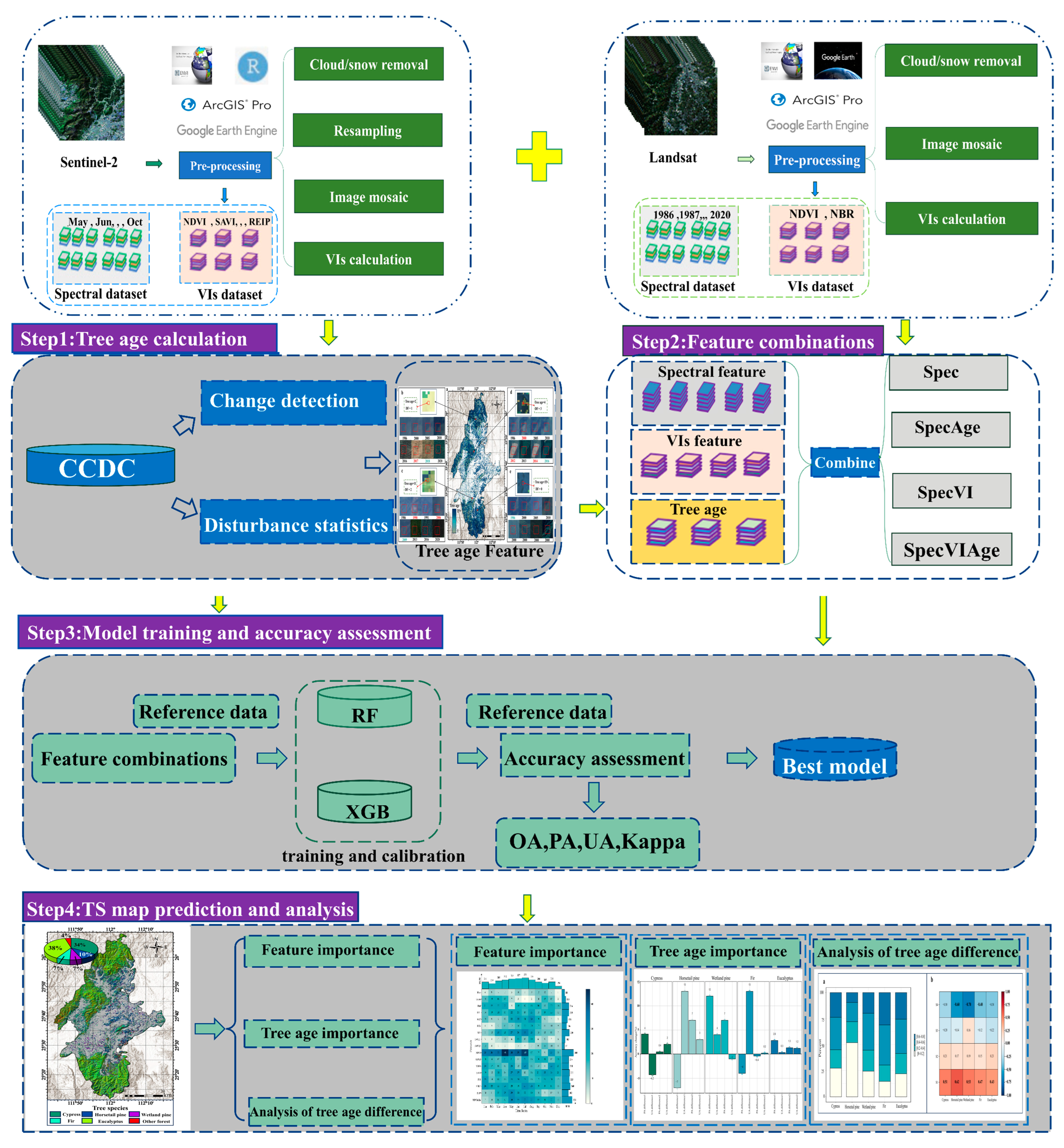
A workflow (Figure 2) was established to map the tree species, encompassing the following steps: (1) tree age calculation; (2) feature combinations; (3) model training and accuracy assessment; and (4) tree species mapping.
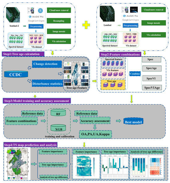
Figure 2.
Workflow of the tree species mapping approaches. TS: tree species. VIs: Vegetation indexes. CCDC: Continuous Change Detection and Classification algorithm. Spec: spectral band, SpecAge: spectral band combined with tree age feature, SpecVI: spectral band combined with spectral index, SpecVIAge: spectral band combined with spectral index and tree age feature. OA: overall accuracy. UA: user’s accuracy. PA: producer’s accuracy. Kappa: kappa coefficient.
3.1. Calculate Forest Age Feature
Limited studies on estimating forest age have primarily employed regression and growth model prediction methods [40,41]. However, these methods necessitate detailed tree age sample data or strict tree species growth equations, posing significant challenges [42]. Fortunately, satellite-based remote sensing technology provides a cost-effective method to estimate forest age by using change detection algorithms [43]. These algorithms offer promise for generating transparent and systematic tree age estimates over large areas [37,41]. In this study, the Continuous Change Detection and Classification (CCDC) algorithm was employed to estimate tree age. CCDC is known for its robust performance and capability to provide continuous monitoring of changes, enabling the analysis of land cover changes over time [42,45]. It utilizes the long time series Landsat data and NDVI and NBR data to establish the linear fitting model for each pixel based on Ordinary Least Squares (OLS), and the difference between predicted values and actual observations is calculated. If this difference exceeds three times the Root Mean Square Error (RMSE) for six consecutive times or more during the detection, the pixel is determined to be disturbed. At this point, breakpoints may appear in the time series curves of NDVI and NBR obtained from model fitting. Since NDVI and NBR are used simultaneously as inputs for the CCDC algorithm in this study but have different sensitivities to forests, the timing of breakpoints may diverge. To address this issue, this study analyzed the change detection results corresponding to the locations of all detected breakpoints. The ‘chiSquareProbability’ band from the results was extracted, which represents the probability of occurrence for each breakpoint. We compared the probabilities of occurrence for all breakpoints in the NDVI and NBR time series curves. The times corresponding to breakpoints with high probabilities of occurrence were recorded as disturbance times [45,46,47]. Given that the disturbance time of a forest often does not align with the planting years, this discrepancy arises from the likelihood that the forest may exist in an “idle” state for a certain duration post-disturbance. For instance, the forest might not be promptly replanted after the disturbance event, causing the area to be classified as grassland or wasteland before the subsequent planting activity. Based on this consideration, it is wrong to determine the time of forest disturbance as the starting time of tree age (i.e., planting time).
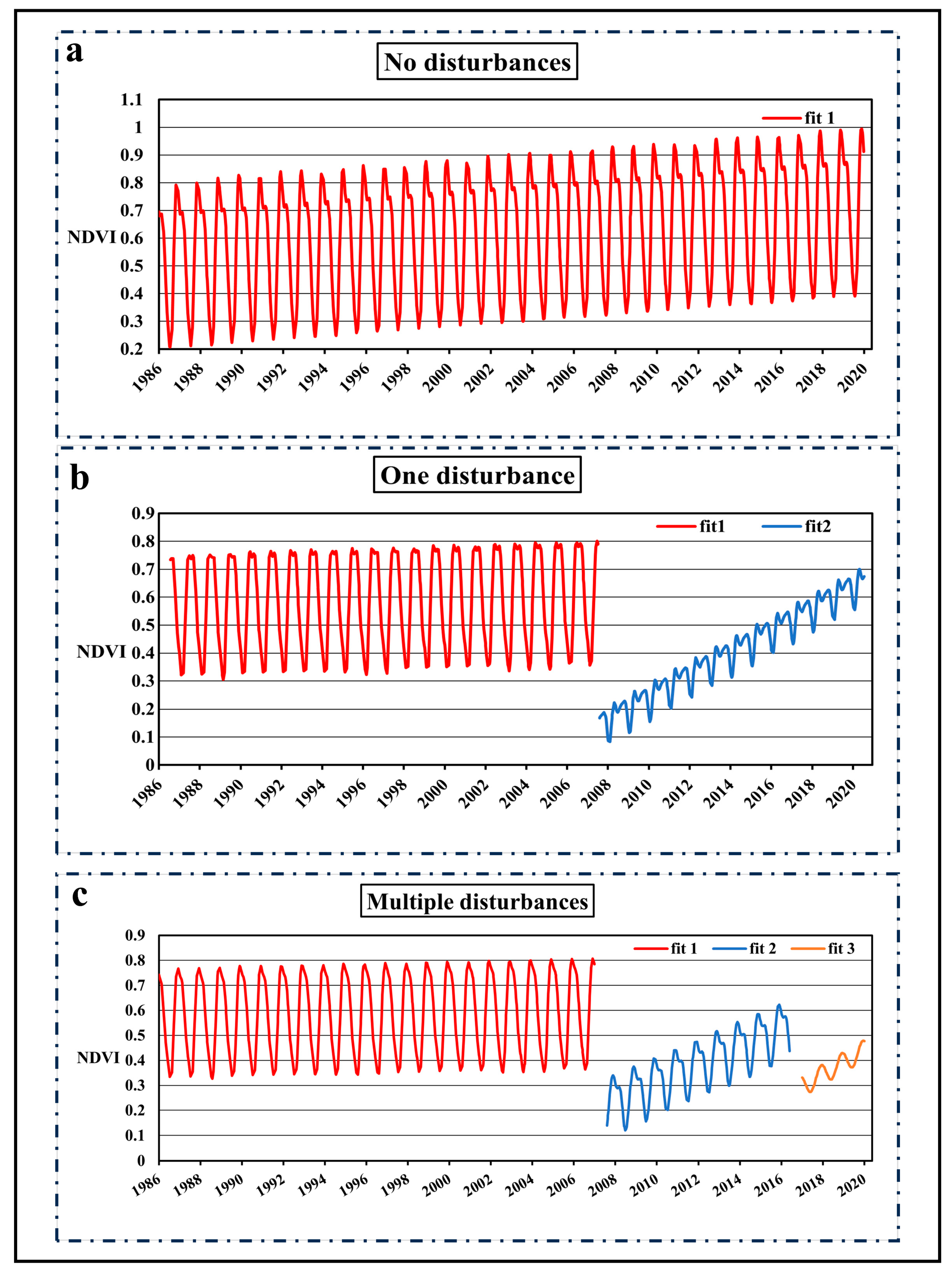
To remove false detection, the decision rules set by Du et al. to determine the planting year of global plantations [41] were imitated: (1) the duration of the segment should be greater than 1 year; and (2) the increment of fitted observation value in the segment should be greater than 0.2. When the segment met these conditions, the time corresponding to the first vertex was recorded as the planting year. When determining the planting year, generally, three scenarios may arise:
For pixels with no disturbances in the entire time series (Figure 3a), their age was set to 35+ (greater than or equal to 2020–1986).

Figure 3.
Example of forest NDVI time series curves with different disturbance frequencies: (a) represents no disturbance; (b) represents one disturbance; (c) represents multiple disturbances. fit1–3 represent each continuous time series curve. In subplot a, fit1 represents the time series fitting curve of NDVI under undisturbed conditions. In subplot b, fit1 and fit2 represent the time series fitting curves of NDVI before and after a disturbance event, with fit1 being before the disturbance and fit2 after. In subplot b, fit1, fit2, and fit3 represent the time series fitting curves of NDVI before and after multiple disturbance events. Examples of time series curves based on NBR under different disturbance frequencies can be shown in Figure S1.
For pixels with only one disturbance, their age was calculated as 2020 minus the planting year (the planting year in Figure 3b is 2008).
For pixels with multiple disturbances, their age was calculated as 2020 minus the planting year after the final disturbance (the planting year in Figure 3c is 2015).
This section employed the ‘ccdcUtilities’ library within the GEE platform to implement the CCDC algorithm. After applying the CCDC algorithm and performing the necessary mathematical processing, a raster image representing the tree age was generated. The values in this image range from 1 to 35+. Next, precision validation of the tree age calculation results was required. The validation method involved randomly selecting 1000 points from the tree age results. Through visual interpretation in GEE using historical images, the fitting degree between the actual recovery time and the predicted recovery time for all points was analyzed. Evaluation metrics included R2 and RMSE [41].
3.2. Classification Model
In this study, two machine learning algorithms, random forest (RF) and extreme gradient boosting (XGB), were employed for tree species classification. RF is a robust integrated classification algorithm that combines multiple decision trees. By aggregating the results through voting or averaging from multiple weak classifiers, the RF model achieves high accuracy and generalization performance. It is particularly well-suited for handling high-dimensional and multicollinear data. Two crucial hyperparameters were considered in our RF classifier: the number of trees (n_tree) and the maximum depth of each tree (max_depth). XGB is a gradient tree boosting algorithm known for its efficiency, flexibility, and versatility. It has gained widespread popularity in various data science fields. In our study, the performance of the XGB algorithm was controlled using several key hyperparameters, such as the number of trees (nrounds), the learning rate (eta), and the depth per tree (max_depth).
To validate whether tree age can improve classification accuracy, we established four different combinations of classification features for training and evaluating the models. Four independent classification models for each algorithm were generated:
- Spec: This model relies solely on the time series of spectral bands.
- SpecAge: It incorporates both the time series of spectral bands and the tree age feature.
- SpecVI: This model utilizes the time series of spectral bands and spectral indices.
- SpecVIAge: It combines the time series of spectral bands, spectral indices, and the tree age feature.
All models were configured with the same parameter range. Each parameter established combinations according to the predefined step size. For each parameter combination, cross-validation was employed to assess the model’s performance. Ultimately, the parameter combination that exhibited the best performance on the validation set was selected as the final model parameters (Table 4). RF classification was executed using the random forest function within the GEE platform, and the XGB algorithm was implemented in Python 3.7.0 using the XGB package.
Table 4.
Hyperparameters selected for the machine learning algorithms used.
The accuracy evaluation indicators include the user’s accuracy (UA), the producer’s accuracy (PA), overall accuracy (OA), the kappa coefficient, and the confusion matrix [48]. To statistically demonstrate the impact of tree age as a classification feature on the performance of the classification model, the McNemar test was then performed, with the specific formula as follows.
The McNemar test compares the performance of two models on a set of samples by focusing on the disagreement between the models. It is specifically designed for paired nominal data. The test is based on a 2 × 2 contingency table, where the elements are as follows:
The represents the number of samples the first model classified correctly but the second model misclassified; the c represents the number of samples the second model classified correctly but the first model misclassified. This statistic follows a chi-square distribution with 1 degree of freedom. The test evaluates whether the differences in the performance of two models (e.g., with and without the feature of tree age) are statistically significant. A significant result (typically p < 0.05) indicates that the inclusion of tree age significantly affects the model’s classification accuracy.
3.3. Evaluate the Effect of Tree Age Evenness within the Class on Classification Accuracy
The non-uniform distribution of tree age corresponding to each sample polygon across different tree species may impact the final classification results. This is particularly relevant when tree age is used as a classification feature. For instance, consider the case where the age distribution within sample polygons of cypress is uniform, with all trees aged between 10 and 15 years. In contrast, for eucalyptus sample polygons, the age distribution varies significantly, with ages ranging from 1 to 35 years. This variation could lead to differing effects on accuracy improvement for different tree species upon the addition of the tree age feature.
To better assess the evenness of the tree age for each sample polygon within each species, the Simpson index, which measures the uniformity of a population within a class, was calculated for each tree species sample polygons [49]:
Tree age was categorized into distinct intervals with a 5-year span, adhering to the age classification standards for subtropical tree species set by the Chinese forestry department, referred to as “tree age classes”, with a value range of (1–7) [50].Where SI represents the Simpson Index, represents the proportion of each tree age class within the sample, and K denotes the number of tree age classes present in the sample. The higher the Simpson index, the poorer the uniformity of tree age distribution.
Subsequently, the classification results were used to calculate the probability of each sample being classified as its own category (i.e., classification confidence). For each decision tree, its probability output for its own category is denoted as (where represents the index of the tree, and represents the index of the own category). If there are decision trees, the overall output probability of the random forest for the category is given by:
To assess the contribution of samples with different tree age uniformities within each tree species to accuracy in classification, we calculated the correlation between the tree age uniformity of samples within each tree species and their own category probabilities. The Pearson correlation coefficient [51] was used to evaluate the relationship between tree age uniformity and the improvement in classification accuracy.
4. Result
4.1. The Results of Tree Age Feature
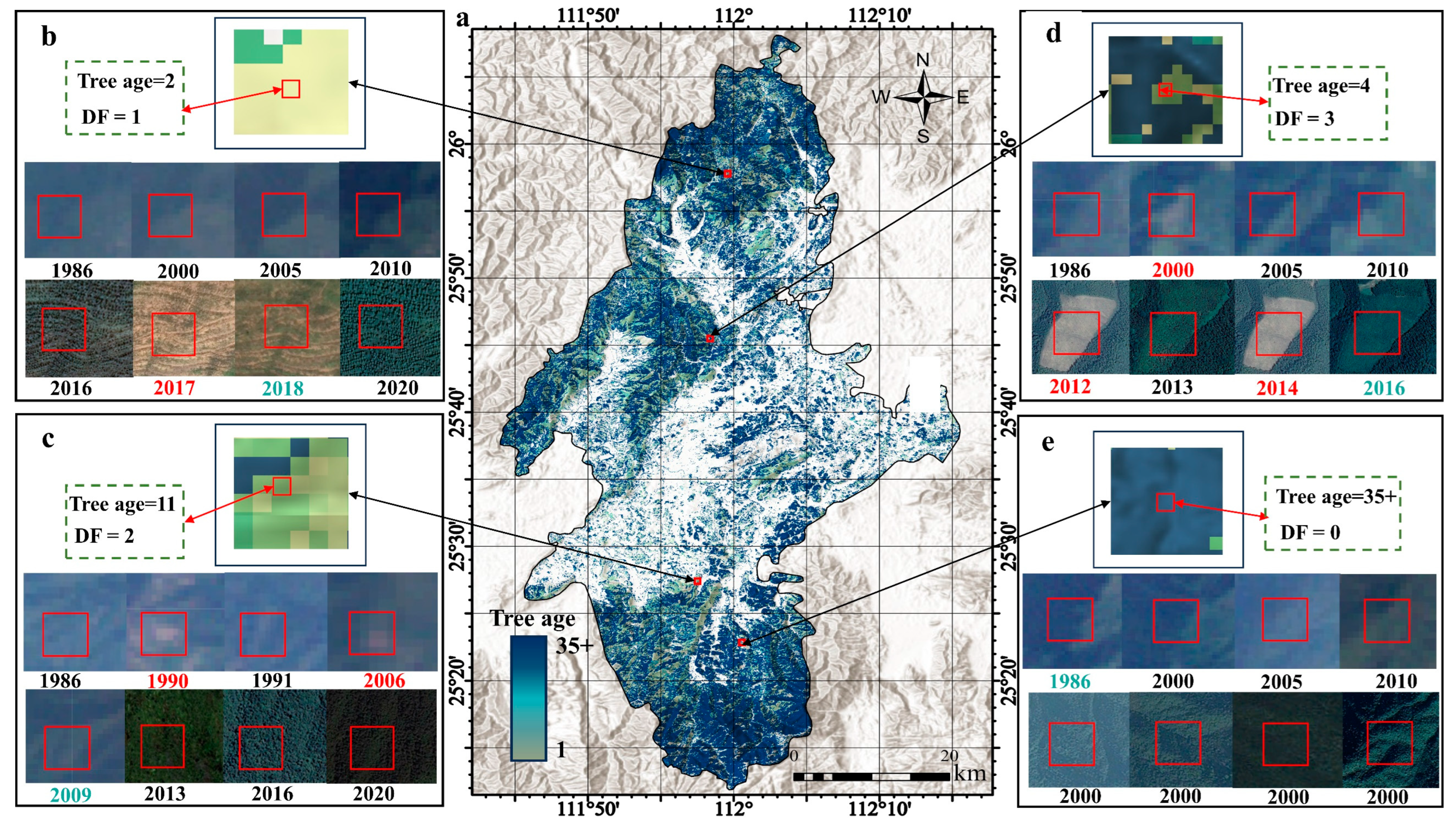
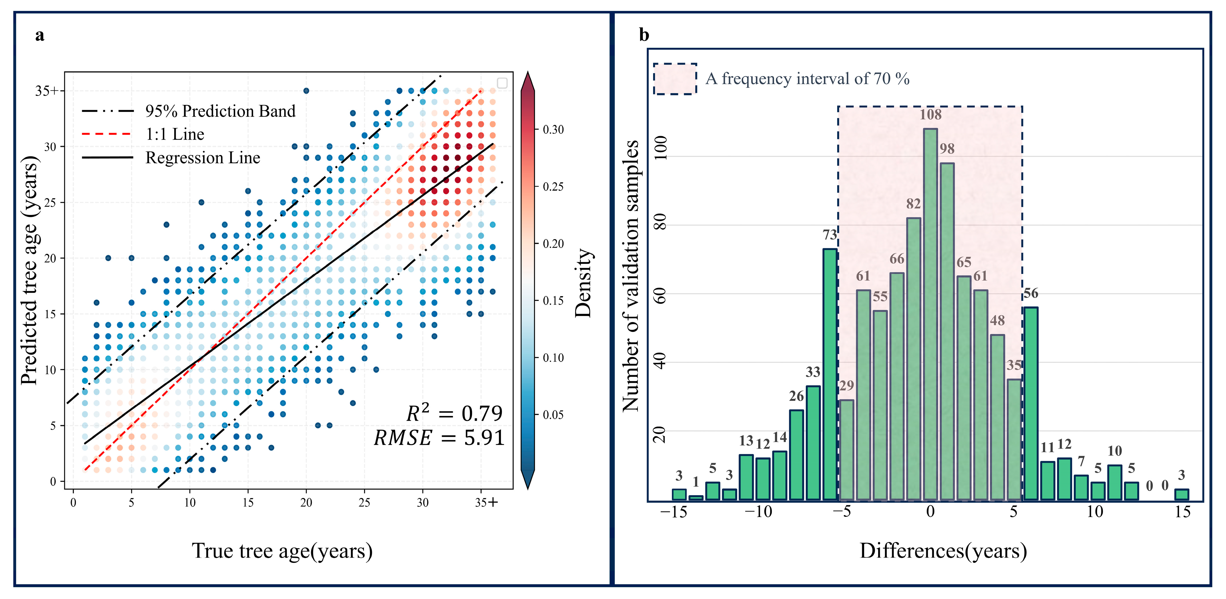
The results reveal a broad range of tree ages in the study area. The mountainous regions to the north and south, with limited human accessibility, exhibit an overall tree age range in the 30–35+ interval (Figure 4a). The southwest and central areas are predominantly composed of younger forests. Through visual interpretation of 1000 validation points, there is satisfactory consistency between the predicted tree age and the actual tree age obtained from historical images (the determination process as shown in the Figure 4b–e), with an of 0.79 and an RMSE of 5.91 (Figure 5a). The difference between the predicted tree age and the actual tree age for verification points was further calculated. The final results indicate that approximately 70% of validation points have a tree age deviation of 5 years (Figure 5b), further confirming the correctness and effectiveness of the method used in this study for tree age calculation.
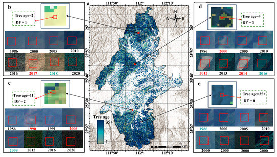
Figure 4.
The results of tree age calculation: (a) represents the spatial distribution of tree age in the study area; (b–e) represent the several examples during the determination of the tree age, DF represents the disturbance frequency, red font indicates disturbance time, and green font represents the planting time obtained through visual interpretation.
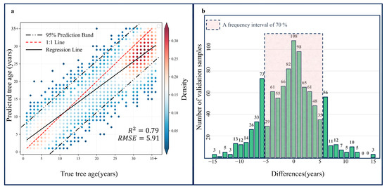
Figure 5.
Validation results of tree age calculation accuracy: (a) represents the fitting degree between predicted tree age and tree age obtained through visual interpretation; (b) represents the statistical results of the difference between the predicted tree age and the actual tree age, the horizontal axis represents the value of the predicted tree age minus the actual tree age.
4.2. Classification Accuracy
After training and predicting with the classification models, the eight models generated through the random forest (RF) and the extreme gradient boosting (XGB) algorithms consistently demonstrated high classification accuracies. As indicated in Table 5, both classification algorithms achieved accuracy rates exceeding 70%, accompanied by Kappa coefficients surpassing 0.55.
Table 5.
The classification accuracy and Kappa coefficients of each model.
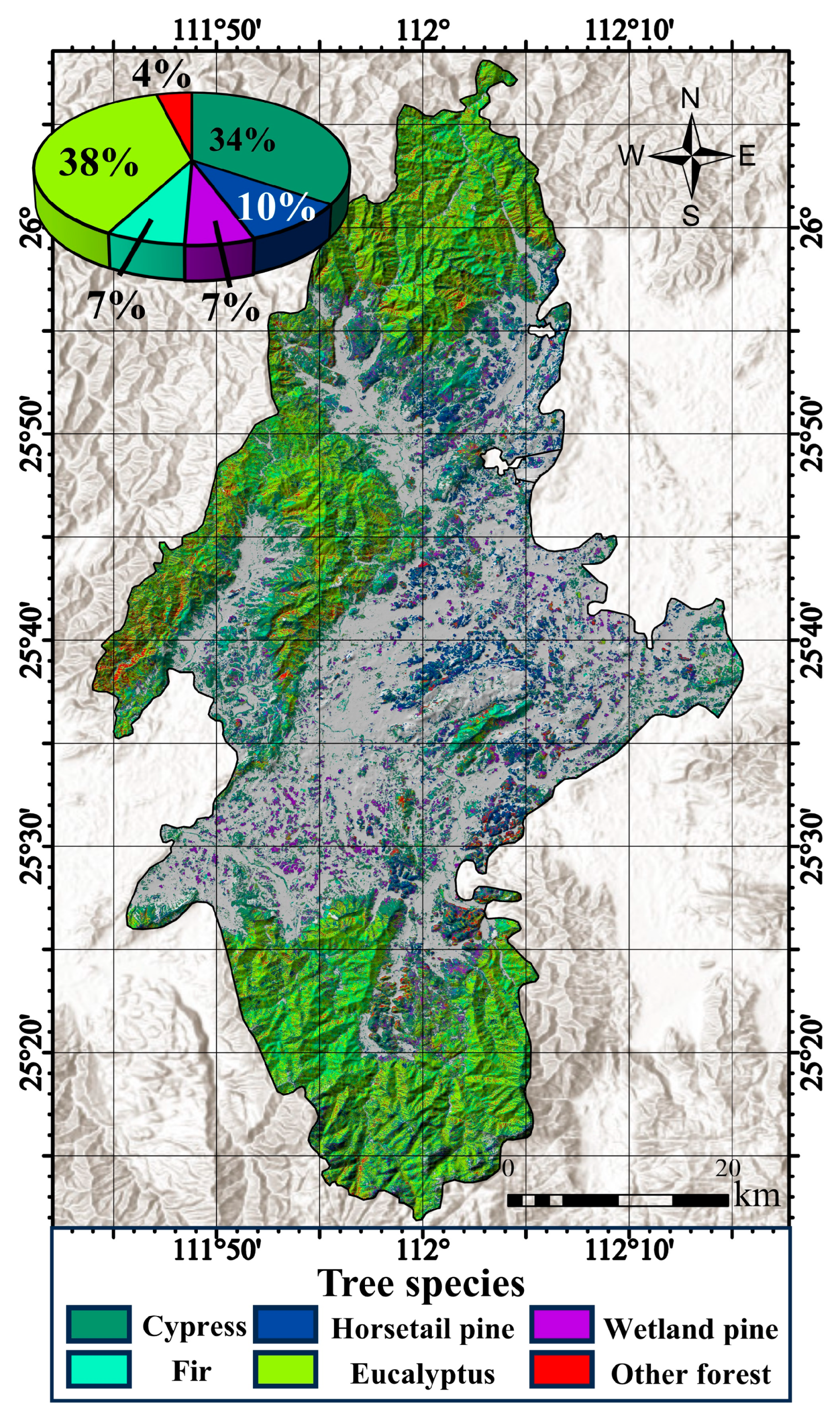
In particular, the models using only time series spectral bands (Spec) in the RF and XGB algorithms achieved OA of 70.1% and 74.2%, respectively, with Kappa coefficients of 0.57 and 0.63. However, when tree age feature was added to these models (SpecAge), the inclusion of tree age feature resulted in a 2.34% and 2.76% increase in OA and a 0.05 and 0.03 increase in the Kappa coefficient, respectively. The higher classification accuracies were achieved by the SpecVIAge models, which utilized spectral bands, spectral indices, and tree age feature. These models attained OA of 75.60% and 78.80%, along with Kappa coefficients of 0.66 and 0.69, respectively. Compared to the SpecVI models, the inclusion of tree age feature led to 2.51% and 2.30% increase in OA, and 0.04 and 0.03 increase in the Kappa coefficients. In summary, the XGB algorithm consistently outperformed the RF algorithm in terms of OA and Kappa coefficient. The addition of the tree age feature improved the classification accuracy, demonstrating the substantial potential of tree age in tree species classification tasks. The SpecVIAge model classification result of the XGB algorithm, which with the highest accuracy, is shown in Figure 6.
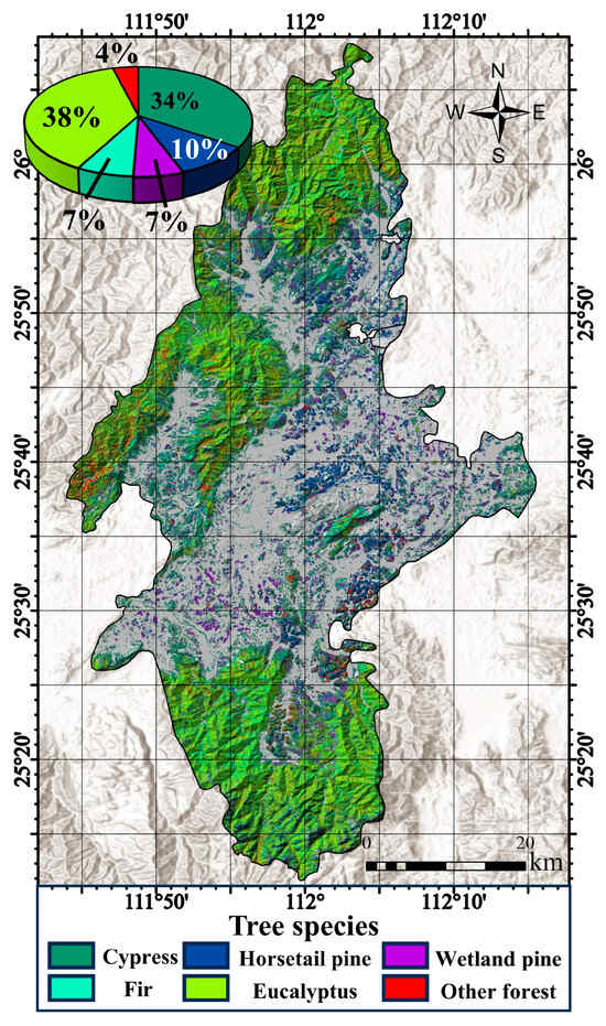
Figure 6.
Tree species classification map based on SpecVIAge model, which belongs to XGB algorithm.
4.3. Importance of Time Series Observations
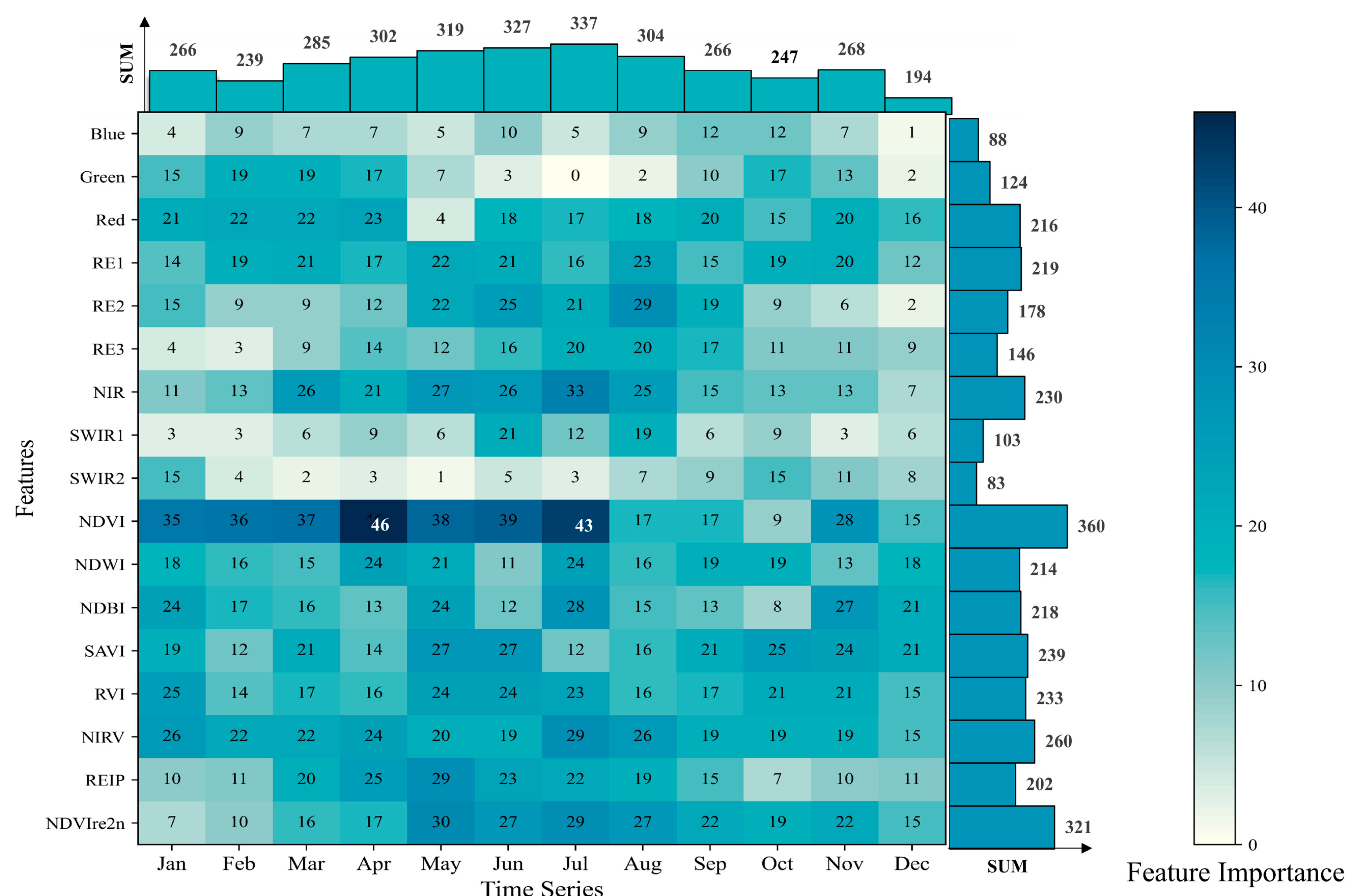
To explore the importance of Sentinel-2 time series data in the task of classifying dominant tree species, the mean decrease in Gini was used to assess feature importance. Classification features demonstrated different distributions of importance in temporal and spectral domains (Figure 7). From the perspective of the spectral distribution of feature importance, NDVI demonstrated the highest feature importance, with features like NDVIre2n and NIRV also exhibiting strong significance. Overall, the contribution of spectral indices was more prominent than spectral bands.

Figure 7.
Feature importance of the SpecVIAge model based on the XGB algorithm. The horizontal and vertical histograms represent the cumulative sum of feature importance based on both spectral and temporal aspects. For months with multiple images, the importance of each feature is presented in the form of averages.
For temporal distribution, the importance of many features remained consistently high over a certain period; for instance, NDVI consistently exhibited remarkable importance over seven consecutive months, confirming the predictive advantage of time series data compared to classification methods based on a single or few images. All features for each month contributed to the classification, but those acquired during the period from April to August showed stronger importance. This implies that tracking phenological changes during this timeframe seems crucial for tree species classification.
4.4. The Importance of Tree Age Feature in Tree Species Classification
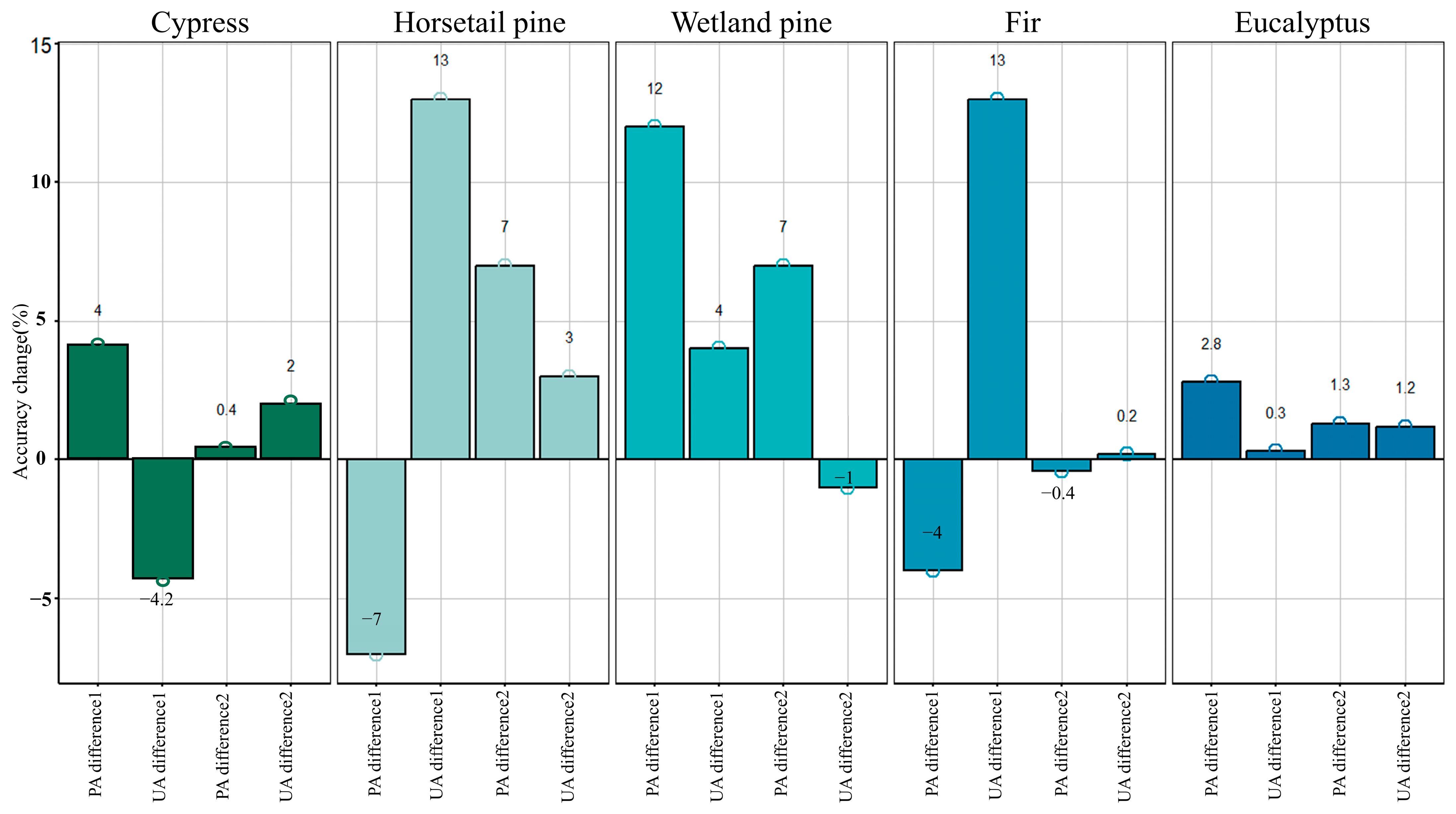
The impact of the tree age feature on tree classification was elucidated by examining the accuracy changes of tree species before and after the introduction of age feature into the classification model (Figure 8). In the SpecAge model, the inclusion of tree age resulted in UA for horsetail pine and fir increasing by 13%, and PA for wetland pine increased by 12%. In SpecVIAge, where tree age still plays an important role, PA for horsetail pine and wetland pine increased by 7%. The accuracy of the remaining tree species also showed varying degrees of improvement.
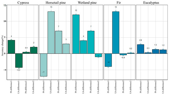
Figure 8.
Accuracy improvement difference of different tree species. PA difference1 = PA of SpecAge—PA of Spec; UA difference1 = UA of SpecAge—UA of Spec; PA difference2 = PA of SpecVIAge—PA of SpecVI; UA difference2 = UA of SpecVIAge—UA of SpecVI.
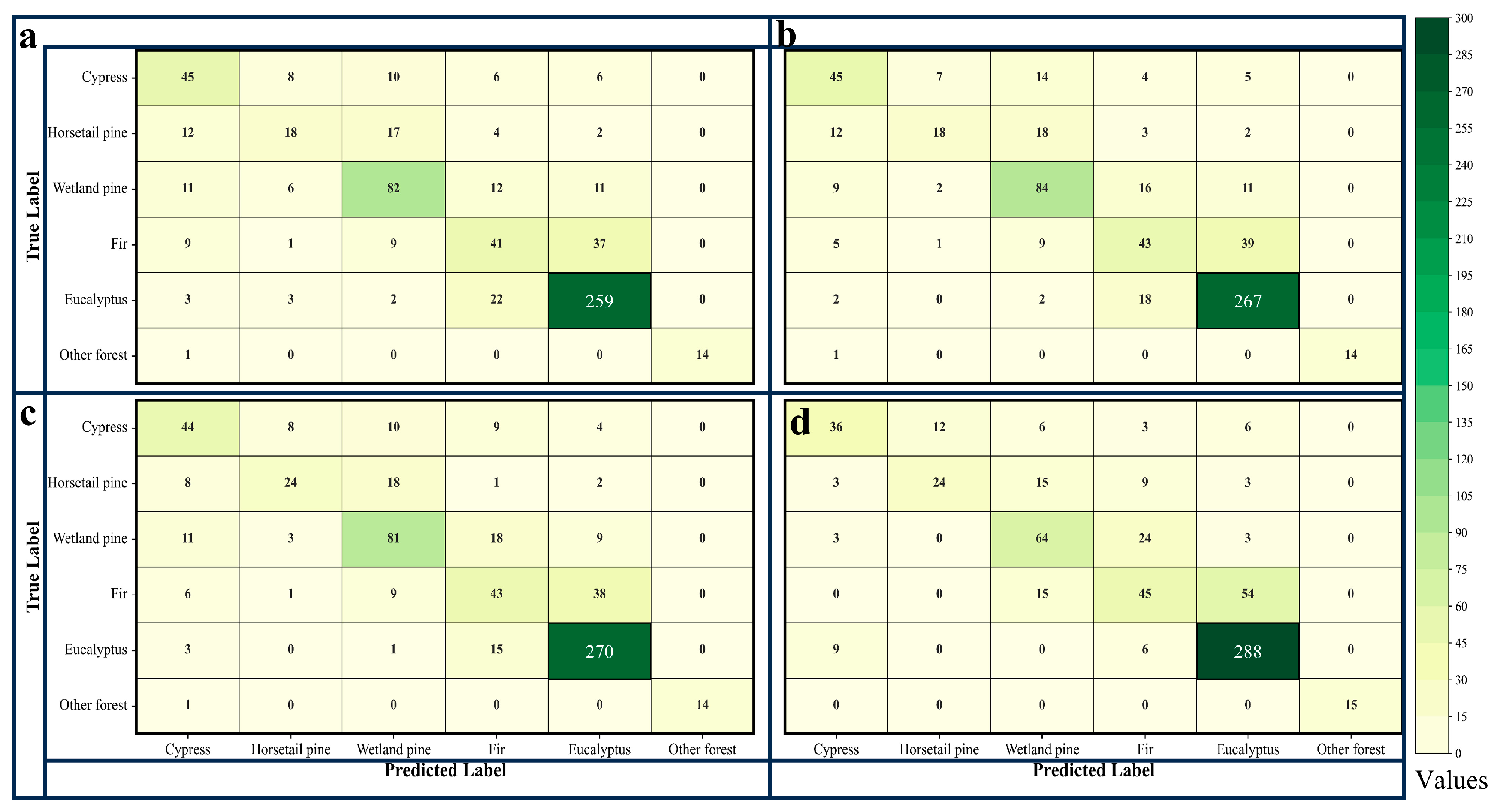
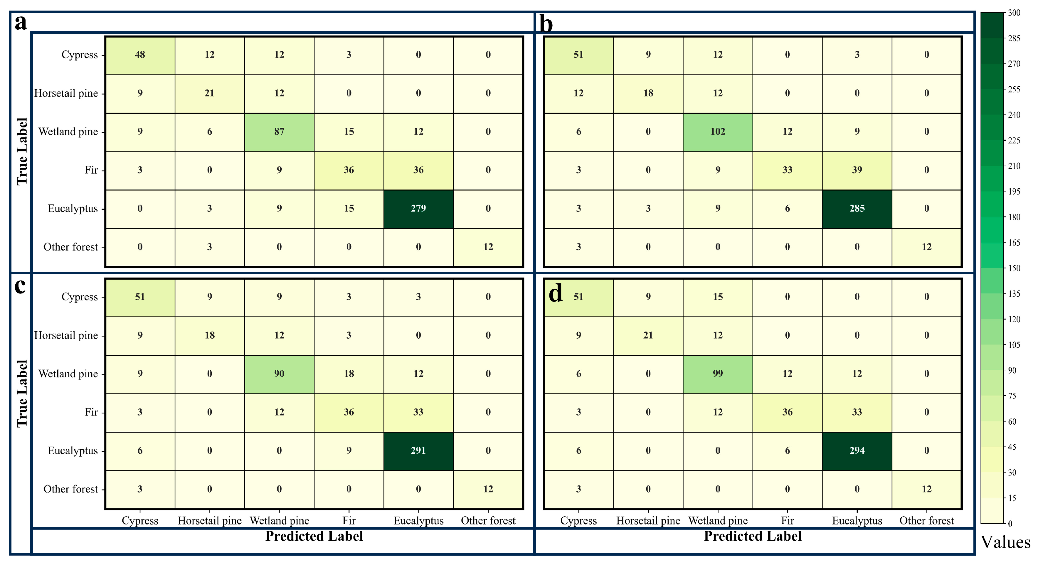
By comparing the confusion matrices of the classification model before and after the addition of tree age (as shown in Figure 9 and Figure 10), we observed that the inclusion of tree age as a classification feature reduced misclassification and omission errors for almost all tree species, with the number of samples on the main diagonal increasing in almost all cases after the addition of tree age. The results of the McNemar test also indicated that the p-values for all models were less than 0.05 (as shown in Table 6). These results confirm that the inclusion of tree age in the classification model improved the model’s performance, effectively enhancing the accuracy of tree species classification, and was statistically significant, but the improvement effect of accuracy was also significantly different for different tree species.

Figure 9.
The confusion matrices for classification models based on the RF algorithm. (a) represents the Spec model; (b) represents the SpecAge model; (c) represents the SpecVI model; (d) represents the SpecVIAge model.
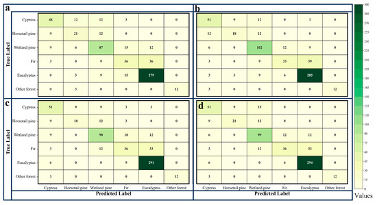
Figure 10.
The confusion matrices for classification models based on the XGB algorithm. (a) represents the Spec model; (b) represents the SpecAge model; (c) represents the SpecVI model; (d) represents the SpecVIAge model.
Table 6.
The p-values from the McNemar test for the models.
4.5. Accuracy Improvement Effect Difference Explanation of Tree Species Classification Based on Tree Age Uniformity
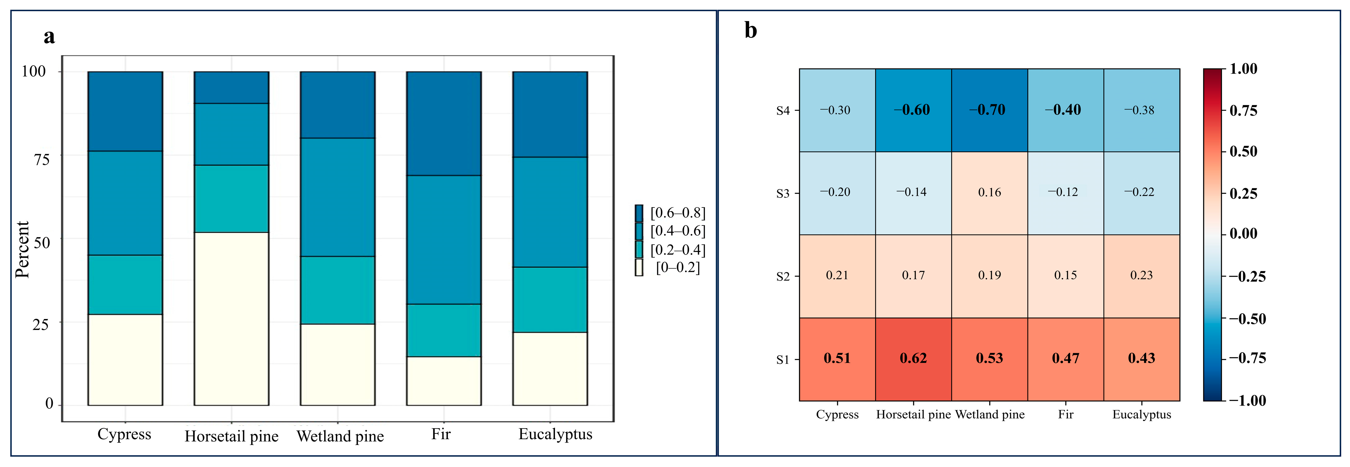
The results of Simpson Index calculations were aggregated with a span of 0.2 (Figure 11a), showing that the proportions of samples with different tree age uniformities vary significantly for each tree species. A higher proportion of samples with high tree age uniformity (such as horsetail pine, 51.8%) corresponds to a more pronounced improvement in classification accuracy. However, when the proportion of samples with low tree age uniformity is too large (such as fir, 31.1%), the effectiveness of tree age features in improving classification accuracy becomes uncertain.

Figure 11.
(a) Represents the percent of each value range of the Simpson index for different tree species sample. (b) Represents the calculation results of the correlation between tree age uniformity and classification confidence; each column represents the correlation between different tree age uniformities and classification confidence within each tree species, S1–S4 represent intervals of different tree age uniformities, corresponding to [0–0.2], [0.2–0.4], [0.4–0.6], and [0.6–0.8], respectively.
Through further correlation analysis, Figure 11b indicates that the higher tree age uniformity has a stronger positive correlation with the sample’s classification confidence. When the tree age uniformity of samples is within the range of [0–0.2], the positive correlation between the sample’s tree age uniformity and classification confidence exceeds 0.4. Specifically, samples of wetland pine exhibit the strongest positive correlation of 0.62. Conversely, as uniformity decreases, a clear negative correlation is evident. For example, within the range of [0.6–0.8] uniformity, almost all tree species show a negative correlation exceeding −0.4. Samples of horsetail pine (−0.6) and wetland pine (−0.7) exhibit strong negative correlations. In other words, while high uniformity in samples can enhance classification accuracy, low uniformity in samples may weaken accuracy. Under the collaborative influence of samples with different tree age uniformities within each tree species, there are variations in the improvement effect on classification accuracy when tree age is involved in the classification process for each tree species.
5. Discussion
In recent years, there has been a notable surge in the utilization of remote sensing data for forest classification. However, the predominant focus in many studies has been on the categorization of broader forest types, such as distinguishing between coniferous and broad-leaved forests. There has been a comparatively limited emphasis on achieving more detailed tree species classification. This study aimed to demonstrate the effectiveness of utilizing time series Sentinel-2 data in conjunction with tree age characteristics to map dominant tree species, achieving an overall accuracy of 78.8%.
The utilization of time series data, adept at capturing persistent phenological information, offers greater predictive advantages compared to classification based solely on single or multi-temporal data. In our study, the classification model employing time series Sentinel-2 spectral data also reached a commendable 74.2% accuracy. However, due to data volume limitations and the consideration of sample acquisition timing within the study area, only 18 images were selected to establish the time series dataset, potentially overlooking the phenological changes in tree species over the years and inter-annual meteorological variations [52,53]. For instance, Hemmerling J. et al. [27] discovered that using Sentinel-2 data over two consecutive years, as opposed to single-year data, led to a class-wise accuracy improvement of up to 15.7%. This presents an area for further exploration in our research.
During the training and prediction phases of the classification model based on the XGB algorithm, we chose to randomly split the sample data into training and validation datasets at a 7:3 ratio. Although models based on the XGB algorithm generally outperform those based on the RF algorithm, the use of random sampling for splitting the sample data might lead to the inclusion of reference samples from the same polygons in both the training and testing datasets. This situation could increase the spatial autocorrelation between the two sets of samples, potentially affecting the performance evaluation of the classification model [54,55]. For instance, Geiß C. et al. [55] have argued that by considering the topological constraints of samples in space and employing spatially disjoint partitioning to separate training and testing samples in space, it is possible to effectively eliminate spatial autocorrelation between the two sets of samples. This limitation needs to be carefully considered in future research.
The integration of remote sensing data with auxiliary data can significantly improve classification accuracy. A notable innovation in this study involves incorporating the tree age feature into the classification model as auxiliary data to improve accuracy. This decision is motivated by the spectral variations observed within the same tree species at different ages. However, in current studies, tree age information is seldom employed as a direct classification feature. Only a few studies combine remote sensing data with stand-related tree age data, such as Mean Diameter at Breast Height (DBH) and canopy height, and have achieved promising results [56,57]. In our study, the inclusion of tree age features improved classification accuracy by 2–3%, providing a straightforward and effective enhancement. Nevertheless, the precision evaluation results highlight a significant issue: the improvement in classification accuracy due to tree age varies among tree species. By analyzing the proportion of samples within different tree age uniformity ranges for each species and calculating the correlation between tree age uniformity and classification confidence, the final results confirm a strong correlation between the improvement in classification accuracy with tree age and the uniformity of samples within each tree species. In other words, in future studies, the criteria for sample selection should not only focus on forest coverage and disturbance but also consider the tree age uniformity of samples.
While our study introduces an innovative concept by utilizing tree age to improve classification accuracy, it does present some limitations. In assessing the planting time of forests, this study achieved high accuracy in predicting tree age by establishing a set of judgment rules, yet instances of misidentification still occurred. The accuracy assessment of tree age indicated that 30% of the validation samples had a deviation of more than five years. This may be due to forests experiencing a period of ‘dormancy’ after disturbance before gradually transitioning into woodland. The planting time decision rules we established cannot guarantee a real-time response to planting events in disturbed areas 100% of the time. This issue can be effectively resolved by incorporating tree age samples obtained from fieldwork. For example, Kai C. et al. [58]developed a tree age prediction framework that combines machine learning algorithms with change detection algorithms, based on field-measured tree age sample data. This approach produced accurate estimates of forest age and effectively eliminated errors in determining planting times. Consequently, this might lead to errors in the predicted tree age for some areas, affecting the performance of tree age in the classification process. Furthermore, considering that the tree age often exceeds 100 years, the data provided by the Landsat satellite, launched in 1972, result in a limited range when using change detection methods to determine tree age. Currently, several scholars have adopted the strategy of change detection coupled with parameter inversion to forecast forest age, aiming to enhance the precision of forest age determination [59,60,61]. Notably, Maltman J. et al. [62]successfully derived a forest age map covering a range of 0–150 years through the integration of remote sensing change detection, regression modeling, and predictions from a forest growth model. This achievement serves as a valuable source of inspiration and reference for our subsequent research endeavors.
6. Conclusions
In this study, Sentinel-2 time series data and tree age features were utilized to identify the dominant tree species, leading to several key findings:
- The superiority of the extreme gradient boosting (XGB) algorithm: The XGB algorithm demonstrated superior classification accuracy and effectiveness, making it more suitable for the classification of dominant tree species in our study. The SpecVIAge model, utilizing the XGB algorithm and incorporating spectral bands, vegetation indices, and tree age, achieved the highest classification accuracy at 78.8%, highlighting the exceptional performance of the XGB algorithm in the classification task.
- The effectiveness of time series data: The Spec model based on the XGB algorithm achieved a classification accuracy of 74.2%, providing strong evidence for the role of time series data in tree species classification. Furthermore, through the analysis of feature importance, most classification features exhibited sustained importance over a period rather than just at individual time steps. The features contributed to the classification every month, with the importance of the features acquired between April and August being particularly strong.
- Effectiveness of the tree age feature: The inclusion of tree age as a feature was found to be an effective means of enhancing tree species classification accuracy. Across both algorithms, in comparison to the model exclusively utilizing spectral bands and vegetation indices, the addition of tree age features resulted in an improvement in classification accuracy ranging from 2% to 3%. This underscores the significant role of tree age in improving classification outcomes.
- Variability in the improvement of classification accuracy: The impact of the tree age feature on classification accuracy varied among different tree species. The difference was attributed to the uniformity of tree age within the samples of the tree species.
Supplementary Materials
The following supporting information can be downloaded at: https://www.mdpi.com/article/10.3390/f15030474/s1, Figure S1: Example of forest NBR time series curves with different disturbance frequencies.
Author Contributions
Conceptualization, B.Y., L.W., X.L. and M.L.; methodology, B.Y. and L.W.; software, B.Y.; validation, B.Y., T.Z. and Y.Z.; formal analysis, B.Y. and L.W.; data curation, B.Y., Y.Z. and T.Z.; writing—original draft preparation, B.Y.; writing—review and editing, B.Y., L.W., X.L., M.L. and Y.Z. All authors have read and agreed to the published version of the manuscript.
Funding
This research was funded by the National Natural Science Foundation of China, grant number 42371326.
Data Availability Statement
The data presented in this study are available on request from the corresponding author.
Acknowledgments
The author would like to express gratitude to the European Space Agency (ESA) and the U.S. Geological Survey (USGS) for providing Sentinel-2 and Landsat data, respectively. Special thanks are also extended to the support from the Google Earth Engine (GEE) platform.
Conflicts of Interest
The authors declare no conflicts of interest.
References
- Xiao, J.; Chevallier, F.; Gomez, C.; Guanter, L.; Hicke, J.A.; Huete, A.R.; Ichii, K.; Ni, W.; Pang, Y.; Rahman, A.F. Remote sensing of the terrestrial carbon cycle: A review of advances over 50 years. Remote Sens. Environ. 2019, 233, 111383. [Google Scholar] [CrossRef]
- Wang, R.; Gamon, J.A. Remote sensing of terrestrial plant biodiversity. Remote Sens. Environ. 2019, 231, 111218. [Google Scholar] [CrossRef]
- Lindner, M.; Maroschek, M.; Netherer, S.; Kremer, A.; Barbati, A.; Garcia-Gonzalo, J.; Seidl, R.; Delzon, S.; Corona, P.; Kolström, M. Climate change impacts, adaptive capacity, and vulnerability of European forest ecosystems. For. Ecol. Manag. 2010, 259, 698–709. [Google Scholar] [CrossRef]
- White, J.C.; Coops, N.C.; Wulder, M.A.; Vastaranta, M.; Hilker, T.; Tompalski, P. Remote sensing technologies for enhancing forest inventories: A review. Can. J. Remote Sens. 2016, 42, 619–641. [Google Scholar] [CrossRef]
- Young, B.; Yarie, J.; Verbyla, D.; Huettmann, F.; Herrick, K.; Chapin, F.S. Modeling and mapping forest diversity in the boreal forest of interior Alaska. Landsc. Ecol. 2017, 32, 397–413. [Google Scholar] [CrossRef]
- Hong, X.; Roosevelt, C.H. Orthorectification of Large Datasets of Multi-scale Archival Aerial Imagery: A Case Study from Türkiye. J. Geovis. Spatial Anal. 2023, 7, 23. [Google Scholar] [CrossRef]
- Yin, H.; Khamzina, A.; Pflugmacher, D.; Martius, C. Forest cover mapping in post-Soviet Central Asia using multi-resolution remote sensing imagery. Sci. Rep. 2017, 7, 1375. [Google Scholar] [CrossRef] [PubMed]
- Shifley, S.R.; He, H.S.; Lischke, H.; Wang, W.J.; Jin, W.; Gustafson, E.J.; Thompson, J.R.; Thompson, F.R.; Dijak, W.D.; Yang, J. The past and future of modeling forest dynamics: From growth and yield curves to forest landscape models. Landsc. Ecol. 2017, 32, 1307–1325. [Google Scholar] [CrossRef]
- Latifi, H.; Heurich, M. Multi-scale remote sensing-assisted forest inventory: A glimpse of the state-of-the-art and future prospects. Remote Sens. 2019, 11, 1260. [Google Scholar] [CrossRef]
- Fassnacht, F.E.; Latifi, H.; Stereńczak, K.; Modzelewska, A.; Lefsky, M.; Waser, L.T.; Straub, C.; Ghosh, A. Review of studies on tree species classification from remotely sensed data. Remote Sens. Environ. 2016, 186, 64–87. [Google Scholar] [CrossRef]
- Kangas, A.; Astrup, R.; Breidenbach, J.; Fridman, J.; Gobakken, T.; Korhonen, K.T.; Maltamo, M.; Nilsson, M.; Nord-Larsen, T.; Næsset, E. Remote sensing and forest inventories in Nordic countries–roadmap for the future. Scand. J. For. Res. 2018, 33, 397–412. [Google Scholar] [CrossRef]
- Van Deventer, H.; Cho, M.; Mutanga, O. Improving the classification of six evergreen subtropical tree species with multi-season data from leaf spectra simulated to WorldView-2 and RapidEye. Int. J. Remote Sens. 2017, 38, 4804–4830. [Google Scholar] [CrossRef]
- Omer, G.; Mutanga, O.; Abdel-Rahman, E.M.; Adam, E. Performance of support vector machines and artificial neural network for mapping endangered tree species using WorldView-2 data in Dukuduku forest, South Africa. IEEE J. Sel. Top. Appl. Earth Obs. Remote Sens. 2015, 8, 4825–4840. [Google Scholar] [CrossRef]
- Immitzer, M.; Atzberger, C.; Koukal, T. Tree species classification with random forest using very high spatial resolution 8-band WorldView-2 satellite data. Remote Sens. 2012, 4, 2661–2693. [Google Scholar] [CrossRef]
- Laurin, G.V.; Puletti, N.; Hawthorne, W.; Liesenberg, V.; Corona, P.; Papale, D.; Chen, Q.; Valentini, R. Discrimination of tropical forest types, dominant species, and mapping of functional guilds by hyperspectral and simulated multispectral Sentinel-2 data. Remote Sens. Environ. 2016, 176, 163–176. [Google Scholar] [CrossRef]
- Grabska, E.; Hostert, P.; Pflugmacher, D.; Ostapowicz, K. Forest stand species mapping using the Sentinel-2 time series. Remote Sens. 2019, 11, 1197. [Google Scholar] [CrossRef]
- Breidenbach, J.; Waser, L.T.; Debella-Gilo, M.; Schumacher, J.; Rahlf, J.; Hauglin, M.; Puliti, S.; Astrup, R. National mapping and estimation of forest area by dominant tree species using Sentinel-2 data. Can. J. For. Res. 2020, 51, 365–379. [Google Scholar] [CrossRef]
- Sudmanns, M.; Tiede, D.; Augustin, H.; Lang, S. Assessing global Sentinel-2 coverage dynamics and data availability for operational Earth observation (EO) applications using the EO-Compass. Int. J. Digit. Earth 2020, 13, 768–784. [Google Scholar] [CrossRef] [PubMed]
- Immitzer, M.; Neuwirth, M.; Böck, S.; Brenner, H.; Vuolo, F.; Atzberger, C. Optimal input features for tree species classification in Central Europe based on multi-temporal Sentinel-2 data. Remote Sens. 2019, 11, 2599. [Google Scholar] [CrossRef]
- Wolter, P.T.; Mladenoff, D.J.; Host, G.E.; Crow, T.R. Using multi-temporal landsat imagery. Photogramm. Eng. Remote Sens. 1995, 61, 1129–1143. [Google Scholar]
- Erinjery, J.J.; Singh, M.; Kent, R. Mapping and assessment of vegetation types in the tropical rainforests of the Western Ghats using multispectral Sentinel-2 and SAR Sentinel-1 satellite imagery. Remote Sens. Environ. 2018, 216, 345–354. [Google Scholar] [CrossRef]
- Nasiri, V.; Beloiu, M.; Darvishsefat, A.A.; Griess, V.C.; Maftei, C.; Waser, L.T. Mapping tree species composition in a Caspian temperate mixed forest based on spectral-temporal metrics and machine learning. Int. J. Appl. Earth Obs. Geoinf. 2023, 116, 103154. [Google Scholar] [CrossRef]
- do Nascimento Bendini, H.; Fonseca, L.M.G.; Schwieder, M.; Körting, T.S.; Rufin, P.; Sanches, I.D.A.; Leitão, P.J.; Hostert, P. Detailed agricultural land classification in the Brazilian cerrado based on phenological information from dense satellite image time series. Int. J. Appl. Earth Obs. Geoinf. 2019, 82, 101872. [Google Scholar] [CrossRef]
- Schwieder, M.; Leitão, P.; Pinto, J.; Teixeira, A.; Pedroni, F.; Sanchez, M.; Bustamante, M.; Hostert, P. Landsat phenological metrics and their relation to aboveground carbon in the Brazilian Savanna. Carbon Balance Manag. 2018, 13, 7. [Google Scholar] [CrossRef] [PubMed]
- Zeng, L.; Wardlow, B.D.; Xiang, D.; Hu, S.; Li, D. A review of vegetation phenological metrics extraction using time-series, multispectral satellite data. Remote Sens. Environ. 2020, 237, 111511. [Google Scholar] [CrossRef]
- Sheeren, D.; Fauvel, M.; Josipović, V.; Lopes, M.; Planque, C.; Willm, J.; Dejoux, J.-F. Tree species classification in temperate forests using Formosat-2 satellite image time series. Remote Sens. 2016, 8, 734. [Google Scholar] [CrossRef]
- Hemmerling, J.; Pflugmacher, D.; Hostert, P. Mapping temperate forest tree species using dense Sentinel-2 time series. Remote Sens. Environ. 2021, 267, 112743. [Google Scholar] [CrossRef]
- Huang, Z.; Zhong, L.; Zhao, F.; Wu, J.; Tang, H.; Lv, Z.; Xu, B.; Zhou, L.; Sun, R.; Meng, R. A spectral-temporal constrained deep learning method for tree species mapping of plantation forests using time series Sentinel-2 imagery. ISPRS J. Photogramm. Remote Sens. 2023, 204, 397–420. [Google Scholar] [CrossRef]
- Abdollahnejad, A.; Panagiotidis, D.; Shataee Joybari, S.; Surový, P. Prediction of dominant forest tree species using quickbird and environmental data. Forests 2017, 8, 42. [Google Scholar] [CrossRef]
- Ferreira, M.P.; Wagner, F.H.; Aragão, L.E.; Shimabukuro, Y.E.; de Souza Filho, C.R. Tree species classification in tropical forests using visible to shortwave infrared WorldView-3 images and texture analysis. ISPRS J. Photogramm. Remote Sens. 2019, 149, 119–131. [Google Scholar] [CrossRef]
- Cheng, K.; Su, Y.; Guan, H.; Tao, S.; Ren, Y.; Hu, T.; Ma, K.; Tang, Y.; Guo, Q. Mapping China’s planted forests using high resolution imagery and massive amounts of crowdsourced samples. ISPRS J. Photogramm. Remote Sens. 2023, 196, 356–371. [Google Scholar] [CrossRef]
- Leckie, D.G.; Gougeon, F.; McQueen, R.; Oddleifson, K.; Hughes, N.; Walsworth, N.; Gray, S. Production of a large-area individual tree species map for forest inventory in a complex forest setting and lessons learned. Can. J. Remote Sens. 2017, 43, 140–167. [Google Scholar] [CrossRef]
- Hermosilla, T.; Bastyr, A.; Coops, N.C.; White, J.C.; Wulder, M.A. Mapping the presence and distribution of tree species in Canada’s forested ecosystems. Remote Sens. Environ. 2022, 282, 113276. [Google Scholar] [CrossRef]
- Broge, N.; Mortensen, J. Deriving green crop area index and canopy chlorophyll density of winter wheat from spectral reflectance data. Remote Sens. Environ. 2002, 81, 45–57. [Google Scholar] [CrossRef]
- McFeeters, S.K. The use of the Normalized Difference Water Index (NDWI) in the delineation of open water features. Int. J. Remote Sens. 1996, 17, 1425–1432. [Google Scholar] [CrossRef]
- Zha, Y.; Gao, J.; Ni, S. Use of normalized difference built-up index in automatically mapping urban areas from TM imagery. Int. J. Remote Sens. 2003, 24, 583–594. [Google Scholar] [CrossRef]
- Bolyn, C.; Michez, A.; Gaucher, P.; Lejeune, P.; Bonnet, S. Forest mapping and species composition using supervised per pixel classification of Sentinel-2 imagery. Biotechnol. Agron. Soc. Environ. 2018, 22, 16. [Google Scholar] [CrossRef]
- Jordan, C.F. Derivation of Leaf-Area Index from Quality of Light on the Forest Floor. Ecology 1969, 50, 663–666. [Google Scholar] [CrossRef]
- Badgley, G.; Field, C.B.; Berry, J.A. Canopy near-infrared reflectance and terrestrial photosynthesis. Sci. Adv. 2017, 3, e1602244. [Google Scholar] [CrossRef]
- Martimort, P.; Fernandez, V.; Kirschner, V.; Isola, C.; Meygret, A. Sentinel-2 MultiSpectral imager (MSI) and calibration/validation. In Proceedings of the 2012 IEEE International Geoscience and Remote Sensing Symposium, Munich, Germany, 22–27 July 2012; pp. 6999–7002. [Google Scholar]
- Du, Z.; Yu, L.; Yang, J.; Xu, Y.; Chen, B.; Peng, S.; Zhang, T.; Fu, H.; Harris, N.; Gong, P. A global map of planting years of plantations. Sci. Data 2022, 9, 141. [Google Scholar] [CrossRef]
- Giannetti, F.; Pecchi, M.; Travaglini, D.; Francini, S.; D’Amico, G.; Vangi, E.; Cocozza, C.; Chirici, G. Estimating VAIA windstorm damaged forest area in Italy using time series Sentinel-2 imagery and continuous change detection algorithms. Forests 2021, 12, 680. [Google Scholar] [CrossRef]
- Cohen, W.B.; Yang, Z.; Healey, S.P.; Kennedy, R.E.; Gorelick, N. A LandTrendr multispectral ensemble for forest disturbance detection. Remote Sens. Environ. 2018, 205, 131–140. [Google Scholar] [CrossRef]
- Yang, J.; Huang, X. The 30 m annual land cover dataset and its dynamics in China from 1990 to 2019. Earth Syst. Sci. Data 2021, 13, 3907–3925. [Google Scholar] [CrossRef]
- Zhu, Z.; Woodcock, C.E. Continuous change detection and classification of land cover using all available Landsat data. Remote Sens. Environ. 2014, 144, 152–171. [Google Scholar] [CrossRef]
- Arévalo, P.; Bullock, E.L.; Woodcock, C.E.; Olofsson, P. A suite of tools for continuous land change monitoring in google earth engine. Front. Clim. 2020, 2, 576740. [Google Scholar] [CrossRef]
- Xiao, Y.; Wang, Q.; Tong, X.; Atkinson, P.M. Thirty-meter map of young forest age in China. Earth Syst. Sci. Data 2023, 15, 3365–3386. [Google Scholar] [CrossRef]
- Story, M.; Congalton, R.G. Accuracy assessment: A user’s perspective. Photogramm. Eng. Remote Sens. 1986, 52, 397–399. [Google Scholar]
- Simpson, E.H. Measurement of diversity. Nature 1949, 163, 688. [Google Scholar] [CrossRef]
- Grabska, E.; Frantz, D.; Ostapowicz, K. Evaluation of machine learning algorithms for forest stand species mapping using Sentinel-2 imagery and environmental data in the Polish Carpathians. Remote Sens. Environ. 2020, 251, 112103. [Google Scholar] [CrossRef]
- Cohen, I.; Huang, Y.; Chen, J.; Benesty, J.; Benesty, J.; Chen, J.; Huang, Y.; Cohen, I. Pearson correlation coefficient. In Noise Reduction in Speech Processing; Springer: Berlin/Heidelberg, Germany, 2009; pp. 1–4. [Google Scholar]
- Pflugmacher, D.; Cohen, W.B.; Kennedy, R.E. Using Landsat-derived disturbance history (1972–2010) to predict current forest structure. Remote Sens. Environ. 2012, 122, 146–165. [Google Scholar] [CrossRef]
- Zald, H.S.; Ohmann, J.L.; Roberts, H.M.; Gregory, M.J.; Henderson, E.B.; McGaughey, R.J.; Braaten, J. Influence of lidar, Landsat imagery, disturbance history, plot location accuracy, and plot size on accuracy of imputation maps of forest composition and structure. Remote Sens. Environ. 2014, 143, 26–38. [Google Scholar] [CrossRef]
- Ghorbanian, A.; Zaghian, S.; Asiyabi, R.M.; Amani, M.; Mohammadzadeh, A.; Jamali, S. Mangrove Ecosystem Mapping Using Sentinel-1 and Sentinel-2 Satellite Images and Random Forest Algorithm in Google Earth Engine. Remote Sens. 2021, 13, 2565. [Google Scholar] [CrossRef]
- Geiß, C.; Pelizari, P.A.; Schrade, H.; Brenning, A.; Taubenböck, H. On the Effect of Spatially Non-Disjoint Training and Test Samples on Estimated Model Generalization Capabilities in Supervised Classification With Spatial Features. IEEE Geosci. Remote Sens. Lett. 2017, 14, 2008–2012. [Google Scholar] [CrossRef]
- Lu, D.; Moran, E.; Batistella, M. Linear mixture model applied to Amazonian vegetation classification. Remote Sens. Environ. 2003, 87, 456–469. [Google Scholar] [CrossRef]
- Cho, M.A.; Mathieu, R.; Asner, G.P.; Naidoo, L.; Van Aardt, J.; Ramoelo, A.; Debba, P.; Wessels, K.; Main, R.; Smit, I.P. Mapping tree species composition in South African savannas using an integrated airborne spectral and LiDAR system. Remote Sens. Environ. 2012, 125, 214–226. [Google Scholar] [CrossRef]
- Cheng, K.; Chen, Y.; Xiang, T.; Yang, H.; Liu, W.; Ren, Y.; Guan, H.; Hu, T.; Ma, Q.; Guo, Q. A 2020 forest age map for China with 30 m resolution. Earth Syst. Sci. Data 2024, 16, 803–819. [Google Scholar] [CrossRef]
- Diao, J.; Feng, T.; Li, M.; Zhu, Z.; Liu, J.; Biging, G.; Zheng, G.; Shen, W.; Wang, H.; Wang, J. Use of vegetation change tracker, spatial analysis, and random forest regression to assess the evolution of plantation stand age in Southeast China. Ann. For. Sci. 2020, 77, 27. [Google Scholar] [CrossRef]
- Besnard, S.; Koirala, S.; Santoro, M.; Weber, U.; Nelson, J.; Gütter, J.; Herault, B.; Kassi, J.; N’Guessan, A.; Neigh, C. Mapping global forest age from forest inventories, biomass and climate data. Earth Syst. Sci. Data 2021, 13, 4881–4896. [Google Scholar] [CrossRef]
- Schumacher, J.; Hauglin, M.; Astrup, R.; Breidenbach, J. Mapping forest age using National Forest Inventory, airborne laser scanning, and Sentinel-2 data. For. Ecosyst. 2020, 7, 60. [Google Scholar] [CrossRef]
- Maltman, J.C.; Hermosilla, T.; Wulder, M.A.; Coops, N.C.; White, J.C. Estimating and mapping forest age across Canada’s forested ecosystems. Remote Sens. Environ. 2023, 290, 113529. [Google Scholar] [CrossRef]
Disclaimer/Publisher’s Note: The statements, opinions and data contained in all publications are solely those of the individual author(s) and contributor(s) and not of MDPI and/or the editor(s). MDPI and/or the editor(s) disclaim responsibility for any injury to people or property resulting from any ideas, methods, instructions or products referred to in the content. |
© 2024 by the authors. Licensee MDPI, Basel, Switzerland. This article is an open access article distributed under the terms and conditions of the Creative Commons Attribution (CC BY) license (https://creativecommons.org/licenses/by/4.0/).