1. Introduction
Accurate and comprehensive mapping of tree species serves as the foundation for forest resource management and forestry development. It is indispensable for biodiversity conservation and monitoring of forest carbon stocks [
1,
2]. Simultaneously, considering the profound sensitivity of forest ecosystems to climate change, tree species information becomes crucial for assessing the potential ecological impact of future climatic shifts on forest ecosystems [
3]. Historically, conventional fieldwork was the primary approach. However, its application was constrained by survey costs and accessibility issues. This limitation made it challenging to provide a detailed composition of tree species across extensive areas [
4,
5,
6].
Remote sensing technology offers an efficient means of gathering species information, providing valuable insights into their spatial distribution. Additionally, it enables the collection of repeatable data observations across vast geographical areas, effectively meeting the increasing demand for data [
7,
8,
9]. The mapping of forest species using remote sensing data has gained significant attention in recent decades [
10,
11]. Typically, very high-resolution data (VHR) such as Worldview and GF-2 have been employed for detailed tree species mapping [
12,
13]. Nevertheless, due to their high acquisition costs and limited availability, VHR are primarily suitable for tree species classification tasks in smaller regions [
10,
14]. In contrast, medium-resolution multispectral data are typically used for larger geographical areas with complex ecological settings, such as Landsat images and Sentinel-2 images, due to their continuity, affordability, and accessibility features [
15,
16,
17]. A recurring theme in these studies is that classification based on multi-temporal remote sensing data often outperforms single-image-based classification, especially when different vegetation phenology stages are captured [
16,
18,
19,
20,
21]. Markus I. et al. [
19] demonstrated that multi-temporal classification models produce superior results compared to single images, especially when acquired based on phenological stages, showcasing the best classification effectiveness. Similarly, Joseph J. et al. [
21] also found that aligning the collection date of remote sensing images with the phenological stage of tree species in the study area can improve discrimination of the dry deciduous forest class from the rainforest class. This is because different tree species display unique physiological and biochemical characteristics at multiple phenological stages. The spectral separability between tree species is enhanced in different phenological stages, which can be utilized for more accurate mapping of tree species [
22].
However, the classification based on multi-temporal remote sensing data also exposes a notable limitation: the continuous evolution of vegetation phenology may lead to incomplete capture of phenological information due to the sparsity of the data [
18]. To overcome the limitation, the tree species classification method based on time series remote sensing data has gained increasing attention [
23,
24]. This approach utilizes denser data to capture continuous and complete phenological changes, resulting in superior classification results compared to methods relying solely on multi-temporal or single images [
25,
26]. For example, in the tree species mapping task within complex mixed forests, Grabska E. et al. [
16] demonstrated that the main reason for the 5–10% improvement in classification accuracy was the use of time series data. Notably, the launch of the Sentinel-2 satellites in 2015 and 2017 marked a significant advancement in the spatial-temporal resolution of multispectral remote sensing data. The 5-day revisit interval and a spatial resolution of 10–20 m have substantially enhanced land cover identification [
16,
18,
19,
23]. Therefore, the use of Sentinel-2 data for constructing time series can provide more detailed surface observation data, potentially resulting in improved classification accuracy [
23]. Hemmerling J. et al. [
27] utilized Sentinel-2 time series data combined with texture features and environmental data to produce a high-precision map of 17 temperate tree species, which demonstrated the significant contribution of time series images for tree species classification. Huang Z. et al. [
28] extracted the spectrum–temporal features of the Sentinel-2-data-based deep learning approach and applied them to the classification of tree species in plantation. The final results confirmed that the time series data could effectively utilize phenological information to improve the classification accuracy of tree species.
A significant challenge in tree classification based on remote sensing data is the spectral variability exhibited by the same tree species. This variability often arises from the morphological and growth adaptations of tree species to their environments, leading to spectral confusion and affecting classification accuracy [
29,
30,
31]. To address this variability, topographic and climatic data are commonly used as auxiliary information to enhance the classification effect [
30,
31,
32]. For instance, Hermosilla T. et al. [
33] highlighted that incorporating topographic factors as auxiliary classification data can significantly enhance classification accuracy. He emphasized the effectiveness of topographic features in mitigating forest spectral variability. However, one often-overlooked factor is the impact of tree age on spectral characteristics. The same tree species at different ages can exhibit significant spectral variability due to variations in their form and growth. Spectral differences within the same tree species at different ages contribute to classification errors. Hemmerling J. et al. [
27] speculated that dividing the reference samples of the same tree species into subclasses according to tree age might reduce the intra-class variability of the tree species. This viewpoint was supported by Grabska E. et al. [
16], who believed that the effect of tree age on the spectral reflectance of forests would often lead to species differences in reflectance, and the classification errors caused by such differences would not be eliminated even with additional environmental variables such as soil and terrain data. Therefore, the spectral variability within tree species caused by tree age, which has negative effects on forest classification accuracy, must be considered. The confirmation of whether tree age, as a classification feature, can eliminate the classification error of forest tree species remains a question.
Our study aimed to achieve the precise classification of dominant tree species in the study area by utilizing Sentinel-2 time series data along with the tree age feature derived from extensive time series Landsat images. The random forest (RF) and extreme gradient boosting (XGB) algorithms, acknowledged for their exceptional performance, were used to construct classification models based on various feature combinations to verify the effectiveness of tree ages as a classification feature.
3. Methods
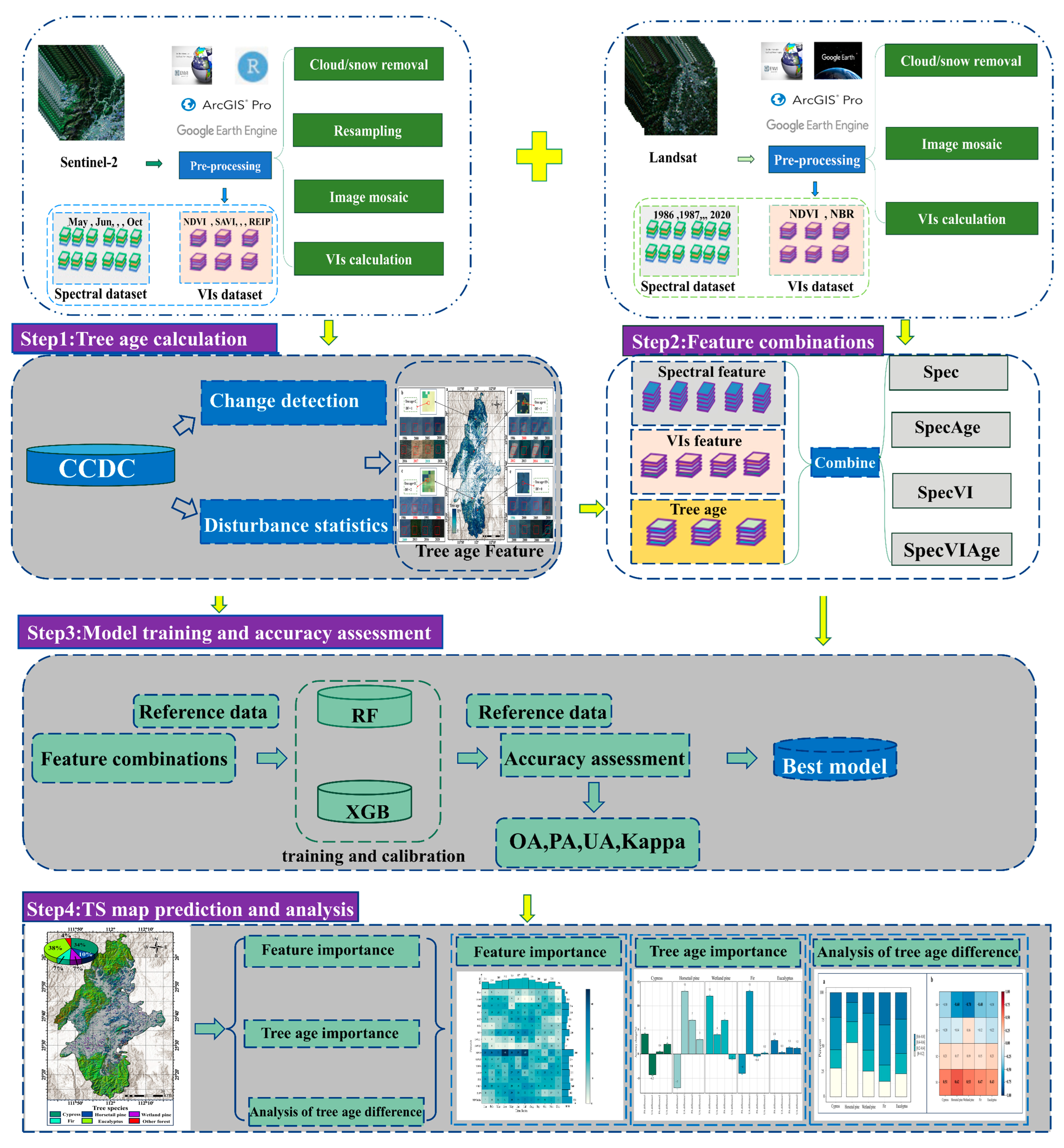
A workflow (
Figure 2) was established to map the tree species, encompassing the following steps: (1) tree age calculation; (2) feature combinations; (3) model training and accuracy assessment; and (4) tree species mapping.
3.1. Calculate Forest Age Feature
Limited studies on estimating forest age have primarily employed regression and growth model prediction methods [
40,
41]. However, these methods necessitate detailed tree age sample data or strict tree species growth equations, posing significant challenges [
42]. Fortunately, satellite-based remote sensing technology provides a cost-effective method to estimate forest age by using change detection algorithms [
43]. These algorithms offer promise for generating transparent and systematic tree age estimates over large areas [
37,
41]. In this study, the Continuous Change Detection and Classification (CCDC) algorithm was employed to estimate tree age. CCDC is known for its robust performance and capability to provide continuous monitoring of changes, enabling the analysis of land cover changes over time [
42,
45]. It utilizes the long time series Landsat data and NDVI and NBR data to establish the linear fitting model for each pixel based on Ordinary Least Squares (OLS), and the difference between predicted values and actual observations is calculated. If this difference exceeds three times the Root Mean Square Error (RMSE) for six consecutive times or more during the detection, the pixel is determined to be disturbed. At this point, breakpoints may appear in the time series curves of NDVI and NBR obtained from model fitting. Since NDVI and NBR are used simultaneously as inputs for the CCDC algorithm in this study but have different sensitivities to forests, the timing of breakpoints may diverge. To address this issue, this study analyzed the change detection results corresponding to the locations of all detected breakpoints. The ‘chiSquareProbability’ band from the results was extracted, which represents the probability of occurrence for each breakpoint. We compared the probabilities of occurrence for all breakpoints in the NDVI and NBR time series curves. The times corresponding to breakpoints with high probabilities of occurrence were recorded as disturbance times [
45,
46,
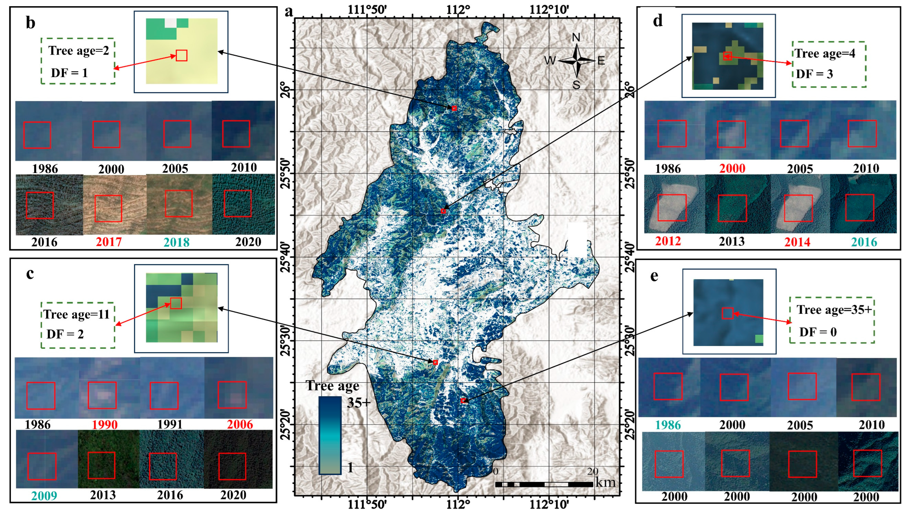
47]. Given that the disturbance time of a forest often does not align with the planting years, this discrepancy arises from the likelihood that the forest may exist in an “idle” state for a certain duration post-disturbance. For instance, the forest might not be promptly replanted after the disturbance event, causing the area to be classified as grassland or wasteland before the subsequent planting activity. Based on this consideration, it is wrong to determine the time of forest disturbance as the starting time of tree age (i.e., planting time).
To remove false detection, the decision rules set by Du et al. to determine the planting year of global plantations [
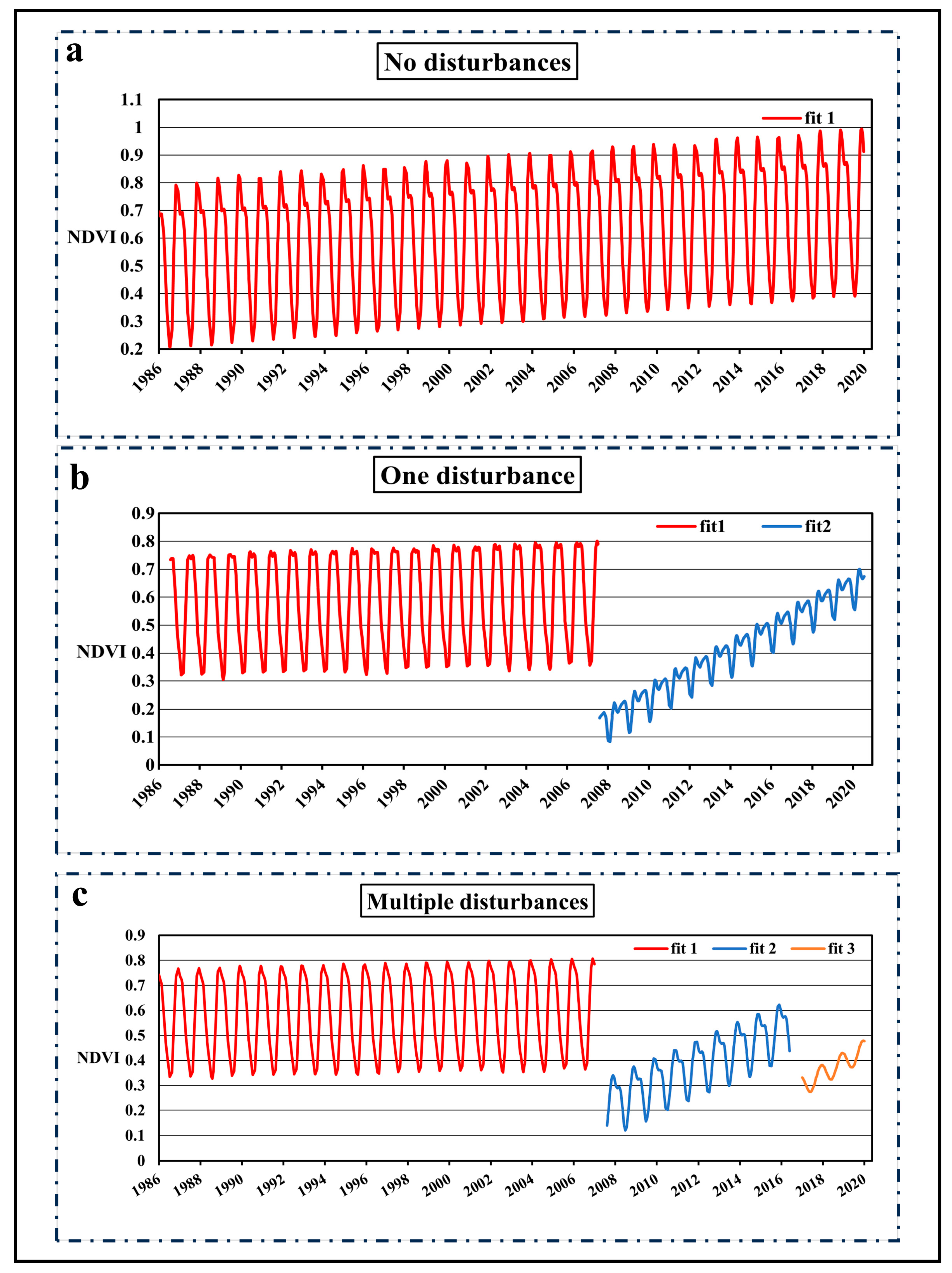
41] were imitated: (1) the duration of the segment should be greater than 1 year; and (2) the increment of fitted observation value in the segment should be greater than 0.2. When the segment met these conditions, the time corresponding to the first vertex was recorded as the planting year. When determining the planting year, generally, three scenarios may arise:
For pixels with no disturbances in the entire time series (
Figure 3a), their age was set to 35+ (greater than or equal to 2020–1986).
For pixels with only one disturbance, their age was calculated as 2020 minus the planting year (the planting year in
Figure 3b is 2008).
For pixels with multiple disturbances, their age was calculated as 2020 minus the planting year after the final disturbance (the planting year in
Figure 3c is 2015).
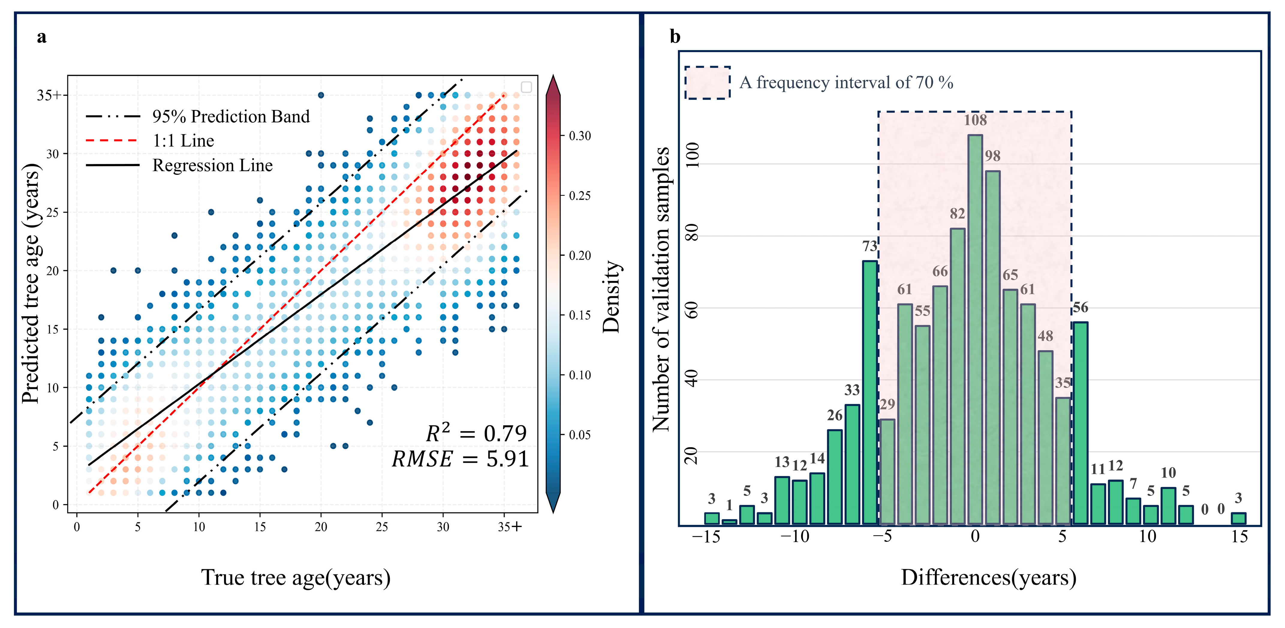
This section employed the ‘ccdcUtilities’ library within the GEE platform to implement the CCDC algorithm. After applying the CCDC algorithm and performing the necessary mathematical processing, a raster image representing the tree age was generated. The values in this image range from 1 to 35+. Next, precision validation of the tree age calculation results was required. The validation method involved randomly selecting 1000 points from the tree age results. Through visual interpretation in GEE using historical images, the fitting degree between the actual recovery time and the predicted recovery time for all points was analyzed. Evaluation metrics included R
2 and RMSE [
41].
3.2. Classification Model
In this study, two machine learning algorithms, random forest (RF) and extreme gradient boosting (XGB), were employed for tree species classification. RF is a robust integrated classification algorithm that combines multiple decision trees. By aggregating the results through voting or averaging from multiple weak classifiers, the RF model achieves high accuracy and generalization performance. It is particularly well-suited for handling high-dimensional and multicollinear data. Two crucial hyperparameters were considered in our RF classifier: the number of trees (n_tree) and the maximum depth of each tree (max_depth). XGB is a gradient tree boosting algorithm known for its efficiency, flexibility, and versatility. It has gained widespread popularity in various data science fields. In our study, the performance of the XGB algorithm was controlled using several key hyperparameters, such as the number of trees (nrounds), the learning rate (eta), and the depth per tree (max_depth).
To validate whether tree age can improve classification accuracy, we established four different combinations of classification features for training and evaluating the models. Four independent classification models for each algorithm were generated:
Spec: This model relies solely on the time series of spectral bands.
SpecAge: It incorporates both the time series of spectral bands and the tree age feature.
SpecVI: This model utilizes the time series of spectral bands and spectral indices.
SpecVIAge: It combines the time series of spectral bands, spectral indices, and the tree age feature.
All models were configured with the same parameter range. Each parameter established combinations according to the predefined step size. For each parameter combination, cross-validation was employed to assess the model’s performance. Ultimately, the parameter combination that exhibited the best performance on the validation set was selected as the final model parameters (
Table 4). RF classification was executed using the random forest function within the GEE platform, and the XGB algorithm was implemented in Python 3.7.0 using the XGB package.
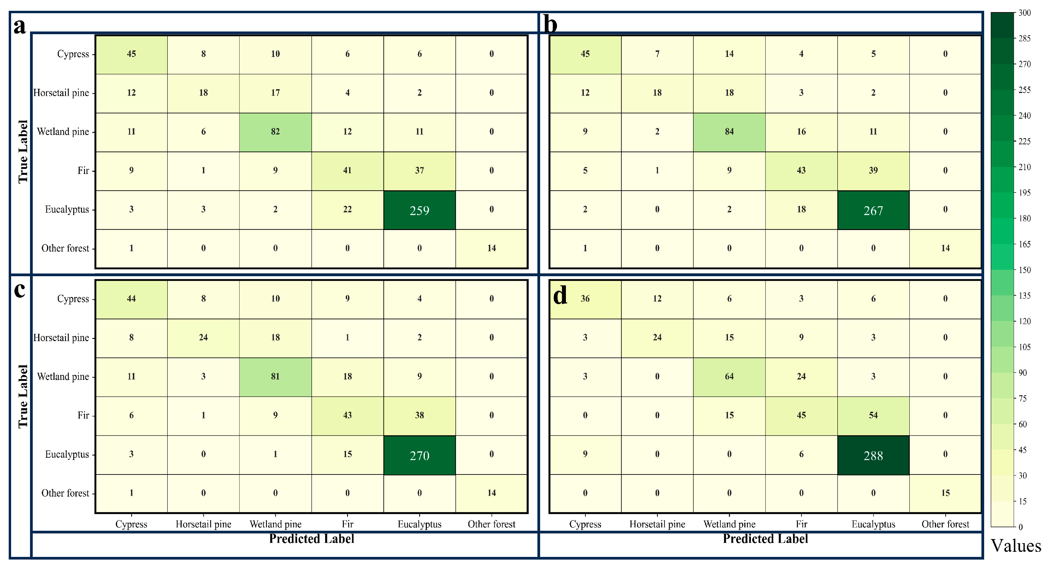
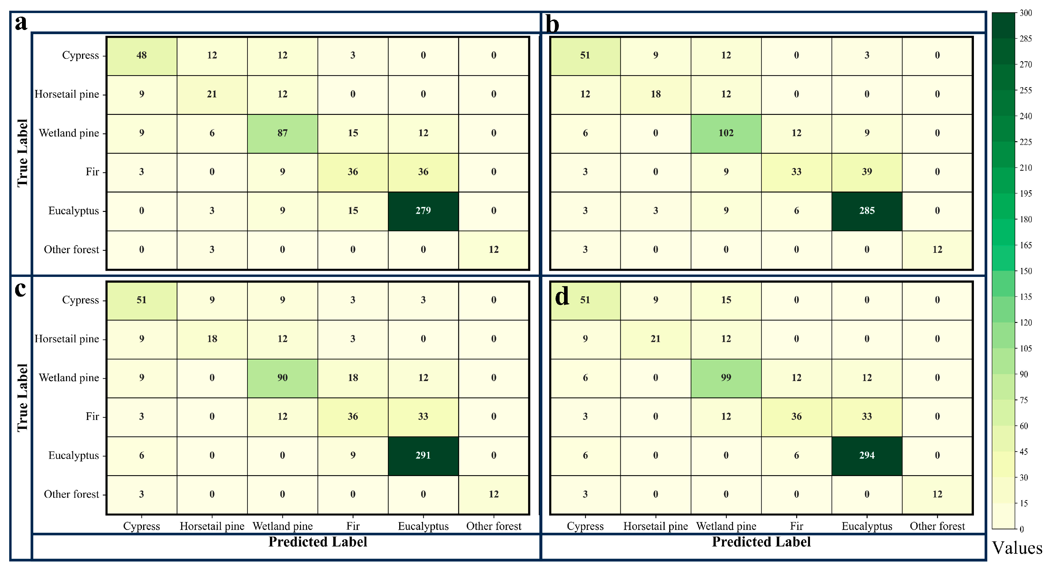
The accuracy evaluation indicators include the user’s accuracy (UA), the producer’s accuracy (PA), overall accuracy (OA), the kappa coefficient, and the confusion matrix [
48]. To statistically demonstrate the impact of tree age as a classification feature on the performance of the classification model, the McNemar test was then performed, with the specific formula as follows.
The McNemar test compares the performance of two models on a set of samples by focusing on the disagreement between the models. It is specifically designed for paired nominal data. The test is based on a 2 × 2 contingency table, where the elements are as follows:
The represents the number of samples the first model classified correctly but the second model misclassified; the c represents the number of samples the second model classified correctly but the first model misclassified. This statistic follows a chi-square distribution with 1 degree of freedom. The test evaluates whether the differences in the performance of two models (e.g., with and without the feature of tree age) are statistically significant. A significant result (typically p < 0.05) indicates that the inclusion of tree age significantly affects the model’s classification accuracy.
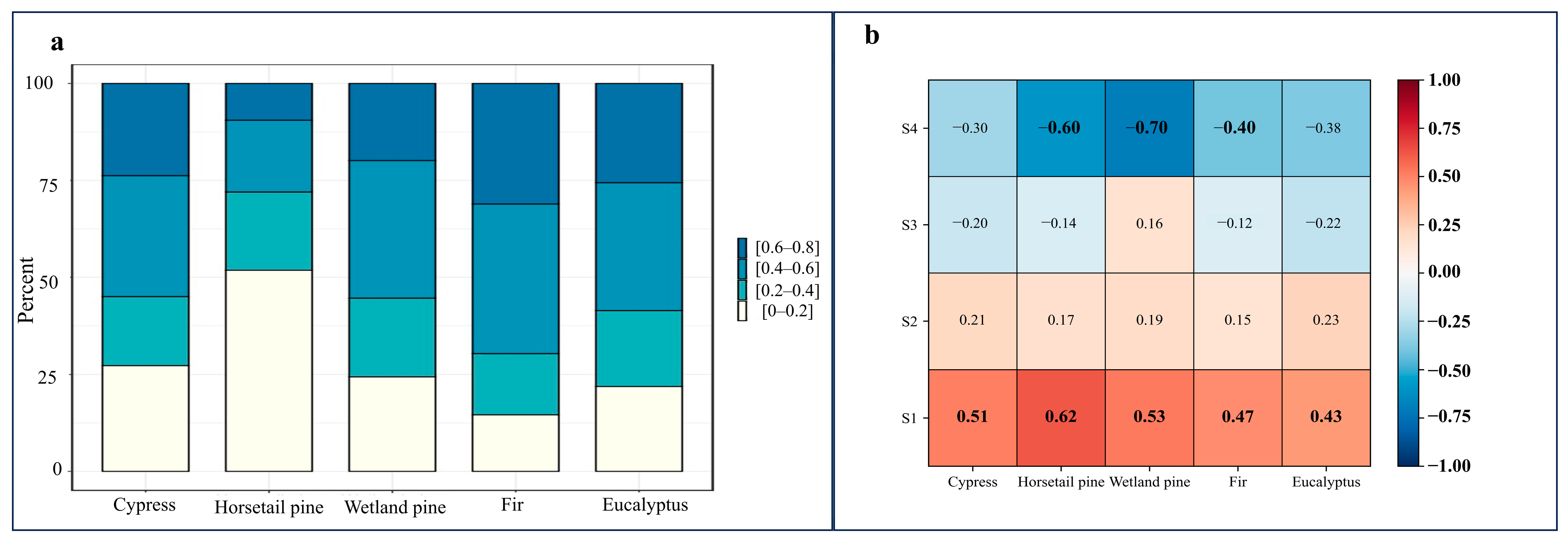
3.3. Evaluate the Effect of Tree Age Evenness within the Class on Classification Accuracy
The non-uniform distribution of tree age corresponding to each sample polygon across different tree species may impact the final classification results. This is particularly relevant when tree age is used as a classification feature. For instance, consider the case where the age distribution within sample polygons of cypress is uniform, with all trees aged between 10 and 15 years. In contrast, for eucalyptus sample polygons, the age distribution varies significantly, with ages ranging from 1 to 35 years. This variation could lead to differing effects on accuracy improvement for different tree species upon the addition of the tree age feature.
To better assess the evenness of the tree age for each sample polygon within each species, the Simpson index, which measures the uniformity of a population within a class, was calculated for each tree species sample polygons [
49]:
Tree age was categorized into distinct intervals with a 5-year span, adhering to the age classification standards for subtropical tree species set by the Chinese forestry department, referred to as “tree age classes”, with a value range of (1–7) [
50].Where SI represents the Simpson Index,
represents the proportion of each tree age class within the sample, and K denotes the number of tree age classes present in the sample. The higher the Simpson index, the poorer the uniformity of tree age distribution.
Subsequently, the classification results were used to calculate the probability of each sample being classified as its own category (i.e., classification confidence). For each decision tree, its probability output for its own category is denoted as
(where
represents the index of the tree, and
represents the index of the own category). If there are
decision trees, the overall output probability of the random forest for the
category is given by:
To assess the contribution of samples with different tree age uniformities within each tree species to accuracy in classification, we calculated the correlation between the tree age uniformity of samples within each tree species and their own category probabilities. The Pearson correlation coefficient [
51] was used to evaluate the relationship between tree age uniformity and the improvement in classification accuracy.
5. Discussion
In recent years, there has been a notable surge in the utilization of remote sensing data for forest classification. However, the predominant focus in many studies has been on the categorization of broader forest types, such as distinguishing between coniferous and broad-leaved forests. There has been a comparatively limited emphasis on achieving more detailed tree species classification. This study aimed to demonstrate the effectiveness of utilizing time series Sentinel-2 data in conjunction with tree age characteristics to map dominant tree species, achieving an overall accuracy of 78.8%.
The utilization of time series data, adept at capturing persistent phenological information, offers greater predictive advantages compared to classification based solely on single or multi-temporal data. In our study, the classification model employing time series Sentinel-2 spectral data also reached a commendable 74.2% accuracy. However, due to data volume limitations and the consideration of sample acquisition timing within the study area, only 18 images were selected to establish the time series dataset, potentially overlooking the phenological changes in tree species over the years and inter-annual meteorological variations [
52,
53]. For instance, Hemmerling J. et al. [
27] discovered that using Sentinel-2 data over two consecutive years, as opposed to single-year data, led to a class-wise accuracy improvement of up to 15.7%. This presents an area for further exploration in our research.
During the training and prediction phases of the classification model based on the XGB algorithm, we chose to randomly split the sample data into training and validation datasets at a 7:3 ratio. Although models based on the XGB algorithm generally outperform those based on the RF algorithm, the use of random sampling for splitting the sample data might lead to the inclusion of reference samples from the same polygons in both the training and testing datasets. This situation could increase the spatial autocorrelation between the two sets of samples, potentially affecting the performance evaluation of the classification model [
54,
55]. For instance, Geiß C. et al. [
55] have argued that by considering the topological constraints of samples in space and employing spatially disjoint partitioning to separate training and testing samples in space, it is possible to effectively eliminate spatial autocorrelation between the two sets of samples. This limitation needs to be carefully considered in future research.
The integration of remote sensing data with auxiliary data can significantly improve classification accuracy. A notable innovation in this study involves incorporating the tree age feature into the classification model as auxiliary data to improve accuracy. This decision is motivated by the spectral variations observed within the same tree species at different ages. However, in current studies, tree age information is seldom employed as a direct classification feature. Only a few studies combine remote sensing data with stand-related tree age data, such as Mean Diameter at Breast Height (DBH) and canopy height, and have achieved promising results [
56,
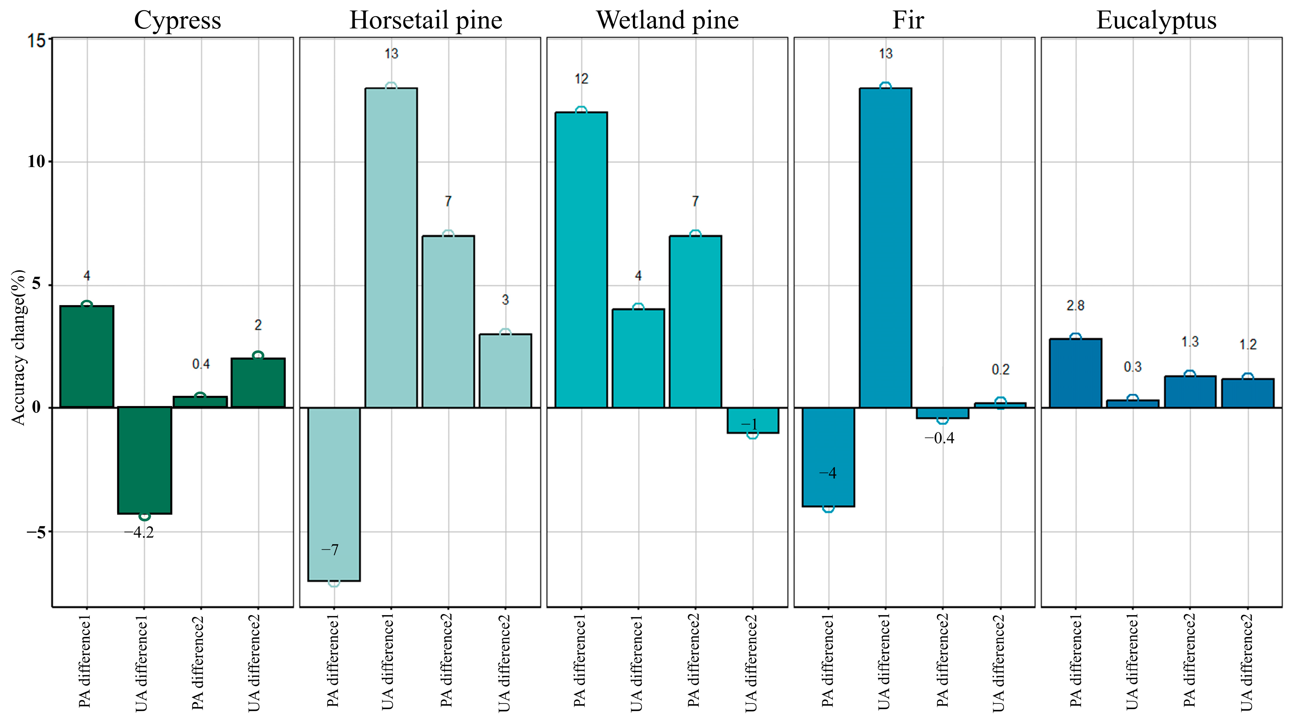
57]. In our study, the inclusion of tree age features improved classification accuracy by 2–3%, providing a straightforward and effective enhancement. Nevertheless, the precision evaluation results highlight a significant issue: the improvement in classification accuracy due to tree age varies among tree species. By analyzing the proportion of samples within different tree age uniformity ranges for each species and calculating the correlation between tree age uniformity and classification confidence, the final results confirm a strong correlation between the improvement in classification accuracy with tree age and the uniformity of samples within each tree species. In other words, in future studies, the criteria for sample selection should not only focus on forest coverage and disturbance but also consider the tree age uniformity of samples.
While our study introduces an innovative concept by utilizing tree age to improve classification accuracy, it does present some limitations. In assessing the planting time of forests, this study achieved high accuracy in predicting tree age by establishing a set of judgment rules, yet instances of misidentification still occurred. The accuracy assessment of tree age indicated that 30% of the validation samples had a deviation of more than five years. This may be due to forests experiencing a period of ‘dormancy’ after disturbance before gradually transitioning into woodland. The planting time decision rules we established cannot guarantee a real-time response to planting events in disturbed areas 100% of the time. This issue can be effectively resolved by incorporating tree age samples obtained from fieldwork. For example, Kai C. et al. [
58]developed a tree age prediction framework that combines machine learning algorithms with change detection algorithms, based on field-measured tree age sample data. This approach produced accurate estimates of forest age and effectively eliminated errors in determining planting times. Consequently, this might lead to errors in the predicted tree age for some areas, affecting the performance of tree age in the classification process. Furthermore, considering that the tree age often exceeds 100 years, the data provided by the Landsat satellite, launched in 1972, result in a limited range when using change detection methods to determine tree age. Currently, several scholars have adopted the strategy of change detection coupled with parameter inversion to forecast forest age, aiming to enhance the precision of forest age determination [
59,
60,
61]. Notably, Maltman J. et al. [
62]successfully derived a forest age map covering a range of 0–150 years through the integration of remote sensing change detection, regression modeling, and predictions from a forest growth model. This achievement serves as a valuable source of inspiration and reference for our subsequent research endeavors.


