Object-Oriented Convolutional Neural Network for Forest Stand Classification Based on Multi-Source Data Collaboration

Abstract

Accurate classification of forest stand is crucial for protection and management needs. However, forest stand classification remains a great challenge because of the high spectral and textural similarity of different tree species. Although existing studies have used multiple remote sensing data for forest identification, the effects of different spatial resolutions and combining multi-source remote sensing data for automatic complex forest stand identification using deep learning methods still require further exploration. Therefore, this study proposed an object-oriented convolutional neural network (OCNN) classification method, leveraging data from Sentinel-2, RapidEye, and LiDAR to explore classification accuracy of using OCNN to identify complex forest stands. The two red edge bands of Sentinel-2 were fused with RapidEye, and canopy height information provided by LiDAR point cloud was added. The results showed that increasing the red edge bands and canopy height information were effective in improving forest stand classification accuracy, and OCNN performed better in feature extraction than traditional object-oriented classification methods, including SVM, DTC, MLC, and KNN. The evaluation indicators show that ResNet_18 convolutional neural network model in the OCNN performed the best, with a forest stand classification accuracy of up to 85.68%.

1. Introduction

The precise identification of forest stand distribution and tree species types is an important factor in forest stand investigation, playing a crucial role in forest resource planning and management, forest biomass, carbon storage, habitat, and ecosystem assessment, and socio-economic sustainable development [1,2]. Mapping vegetation at the species level can help monitor its growth characteristics and spatial distributions and design specific modeling for different tree species existing in an area [3]. In recent decades, remote sensing technology has continuously developed the dynamic management of forest resources due to its ability to break through the limitations of traditional artificial ground mapping, significantly shorten survey time, and reduce labor intensity and work costs [4]. With the advancement of satellite sensors and computer technology, obtaining increasingly accurate data on forest distribution and tree species types through the collaborative utilization of multi-source remote sensing data and the improvement of classification methods has become an important research direction.

At present, remote sensing data sources used for forest classification include multispectral images, hyperspectral images, and light detection and ranging (LiDAR) data [1,4,5,6]. However, a single data source often fails to provide the spectral, texture, and spatial information required for forest classification at the same time. Therefore, a large number of studies have adopted a collaborative approach of multi-source remote sensing data to solve this problem. There are various ways to combine data: for example, Eisfelder, Liu, and Xu [7,8,9,10] integrated multispectral data; Machala, Dechesne, and Xie [11,12,13] combined multispectral and LiDAR data; Dalponte, Ghost, and Shi [14,15,16] combined hyperspectral and LiDAR data. The above research demonstrates the effectiveness of data collaboration in improving forest classification accuracy. While many studies have used one of the approaches described above, there is a growing body of literature highlighting the benefits of LiDAR data, and ignoring targeted research on spectral data; in particular, there is no specific research on the impact of red edge band fusion on forest classification accuracy. The red edge band is defined as the electromagnetic spectrum range in which the reflectance of the green vegetation spectrum curve changes the most within the range of 690–740 nm, located at the junction of the red and near-infrared bands [17,18]. The appearance of red edges in vegetation is caused by two vegetation characteristics: strong absorption of red light by chlorophyll and strong scattering of near-infrared light within leaves. Through the study of the characteristics of red edges, the growth status of vegetation can be identified. Currently, in addition to hyperspectral sensors with red edge bands, an increasing number of multispectral remote sensing satellites have also designed red edge bands. To date, only several satellites have been launched (RapidEye, WordView-2, Sentinel-2, etc.) that are equipped sensors with red edge bands [19]. Among them, RapidEye is the world’s first multispectral commercial satellite that provides a 710 nm red edge band which is conducive to monitoring vegetation and suitable for agricultural, forestry, and environmental monitoring. RapidEye can provide 5-m spatial resolution image data, which is sufficient for the classification of forest species in this study. Sentinel-2 provides the only data with multiple bands within the red edge range, which is very effective for monitoring vegetation health, and its data are easy to obtain [20]. At present, there are some studies using Sentinel-2 and RapidEye data for forest classification, respectively [21,22,23,24,25,26], but few studies have combined RapidEye with Sentinel-2 to maximize the use of the red edge band. Currently, the multispectral data used for forest classification in collaboration with LiDAR data are mostly those from SPOT5, IKONOS, Landsat, and other data lacking the red edge band, which do not meet the requirements for conducting research on the red edge band in this study. Therefore, this study will combine RapidEye, Sentinel-2, and LiDAR data for forest stand classification.

Moreover, classification methods play a crucial role in influencing the precision of forest stand classification. In terms of classification methods, with the improvement of remote sensing image resolution, the advantages of object-oriented classification have gradually showed up. Not only does it avoid the ‘salt and pepper phenomenon’ of traditional pixel based classification methods, but also, compared with traditional pixel based classification methods that can only use pixel spectral information for classification, object-oriented classification can integrate texture information, geometry, and contextual relationships for classification; consequently, it finds effective application in target extraction and land classification [27,28,29,30,31,32]. Stands are independent and distributed in patches, so the object-oriented method has advantages in forest areas. The most commonly used object-oriented classification methods include K-nearest neighbor (KNN), decision tree classification (DTC), maximum likelihood classification (MLC), support vector machine (SVM), etc. However, these methods require manually designed classification features, which are highly dependent on human intervention and difficult-to-learn deep features of images to further improve classification accuracy. In addition, the machine learning algorithms used in current research need to further analyze and extract data features and debug algorithms to seek the optimum parameters [32], resulting in time-consuming, laborious, and poor generalization when extended to different forest types.

Artificial intelligence and machine learning methods can undoubtedly be helpful here [33]. A modern and intensively developing artificial intelligence tool is convolutional neural networks (CNN), which combines neural network technology and deep learning theory. Compared with traditional methods, CNN has a better ability to process images and sequence data, has good learning ability for high-dimensional features, and has better generalization ability. It is widely used to solve various complex multi-level problems, such as fruits classification, face recognition, semantic segmentation, etc. [34,35,36,37,38], and has been successfully applied in remote sensing image scene classification, object detection, image retrieval, and other fields [39,40,41,42]; these classification effects have thus been greatly improved. Generally speaking, the input of convolutional neural networks is image slices, and each image slice is assigned a label, which is highly consistent with object-oriented classification. In the realm of CNN for tree species classification, the majority of research on tree species classification centers on identifying single tree species or individual species within forest stands. There is a relative scarcity of studies addressing the identification of complex forest structures and mixed forests with multiple tree species [43,44,45].

Because of such problems, this study used a combination of RapidEye, Sentinel-2, and LiDAR point cloud data and employed traditional object-oriented classification methods and object-oriented convolutional neural network (OCNN) technology to map complex forest stands. First, to explore the effectiveness of red edge band information and canopy height information in improving forest classification accuracy, RapidEye images were sequentially fused with the two red edge bands of Sentinel-2 to improve the spectral information of RapidEye images. Then, based on this, the canopy height information provided by LiDAR point clouds was fused to further improve classification accuracy.

2. Study Area and Data

2.1. Study Area

The study area is located on Gaofeng Forest Farm, Nanning City, Guangxi Zhuang Autonomous Region, China, with geographical locations ranging from 108°20′ to 108° 27′ E and 22°56′ to 23°1′ N (Figure 1). The total operating area of Gaofeng Forest Farm is over 11.63 square kilometers, with a forest volume of over 5.7 million cubic meters, making it the largest state-owned forest farm in Guangxi. The study area has a subtropical monsoon climate, with an average annual temperature of 21 °C, abundant rainfall, annual precipitation of 1200–1500 mm, average relative humidity of over 80%, and an average frost-free period of 180 days throughout the year. It includes artificial forests, mainly composed of eucalyptus and secondary forests, mainly mixed with coniferous and broad-leaved trees. The research area covers a rich variety of forest types, mainly Illicium verum, Pinus massoniana, Pinus elliottii, eucalyptus grandis, Cunninghamia lanceolata, and broad-leaved tree species. It is a typical subtropical climate forest. Moreover, its forest types, tree species, and stands are some of the most complex in the Chinese region, which provides a good representative sample of the species that grow in the country.

2.2. Data Description

The purpose of this study is to explore the classification potential of red edge band in complex forest stand species and to further improve classification accuracy by utilizing the canopy height information from LiDAR data. Select RapidEye, Sentinel-2A images with red edge bands, and LiDAR data were obtained using unmanned aerial vehicles. By setting up sample plots in the field and conducting field investigations on forest stand types in the study area, we provided a basis for the subsequent production of training samples and verification of classification accuracy.

2.2.1. Remote Sensing Data

The RapidEye image used in the study was obtained on 15 July 2020, and the Sentinel-2A image used in the study was obtained on 18 July 2020, the quality of each is good, with almost no cloud cover. RapidEye images were obtained through purchase, and the purchased RapidEye product level is 3A. It underwent radiation correction, sensor correction, and geometric correction, with a spatial resolution of up to 5 m. One scene image can cover the research area without the need for an image mosaic. From the official website of the European Space Agency (https://scihub.copernicus.eu/dhus/#/home, 10 September 2022), Sentinel-2A images that met the conditions were download. The downloaded product level is L1C, which is an atmospheric apparent reflectance product that has undergone orthophoto correction and geometric precision correction and has not undergone atmospheric correction. Atmospheric correction is performed using the Sen2cor plug-in released by ESA, which is specifically designed to generate L2A-level data. Subsequently, the image was resampled to 10 m and registered with RapidEye to extract the study area through clip. The band characteristics of the two data are shown in

Table 1. Band characteristics of Sentinel-2A and RapidEye: given that different forest types exhibit diverse reflection properties in the red edge band, this band plays a pivotal role in differentiating tree species. Specifically, bands 5, 6, 7, and 8A from Sentinel-2A, along with band 4 from RapidEye, are identified as the red edge bands. These bands are of primary interest to our research.

Sentinel-2A Bands	Central Wavelength (um)	Spatial Resolution (m)	RapidEye Bands	Band Rang (um)	Spatial Resolution (m)
Band 1-Coastal aerosol	0.44	60
Band 2-Blue	0.49	10	Band 1-Blue	440~510	5
Band 3-Green	0.56	10	Band 2-Green	520~590	5
Band 4-Red	0.67	10	Band 3-Red	630~685	5
Band 5-Red Edge1	0.71	20	Band 4-Red Edge	690~730	5
Band 6-Red Edge2	0.74	20
Band 7-Red Edge3	0.78	20	Band 5-NIR	760~850	5
Band 8-NIR	0.84	10
Band 8A-Red Edge4	0.87	20
Band 9-Water vapor	0.95	60
Band 10-SWIR—Cirrus	1.38	60
Band 11-SWIR	1.61	20
Band 12-SWIR	2.19	20

. The study mainly explored the impact of red edge bands for stand classification accuracy, and as shown in Table 1, among the four red edge bands of Sentinel-2A, red edge 1 (RE1) and red edge 3 (RE3) all overlap with the spectral coverage range of RapidEye image; therefore, only red edge 2 (RE2) and red edge 4 (RE4) bands of Sentinel-2A were fused with RapidEye in the following research. In addition, Google Earth images captured at the same period were used to assist in selecting training and validation sample points.

The flight mission was carried out on 20 July 2020, with clear and cloudless weather and wind speeds lower than 3.0 m/s. The mission utilized the airborne observation system of the Chinese Academy of Forestry with an average density of 2.8 points/m², which can provide high-precision digital elevation models (DEMs) and digital surface models (DSMs). During the acquisition process of point cloud data, noise is commonly introduced for various reasons, such as sensor errors and environmental factors. This noise typically manifests as isolated points, drifting points, and redundant points, which can compromise the precision of modeling and information extraction. Therefore, it is essential to remove this noise. Common methods for noise removal include median filtering, mean filtering, Gaussian filtering, statistical filtering, etc. In this study, statistical filtering was employed to remove noise. Specifically, for each point in the point cloud, the average value and standard deviation of points within a certain radius were calculated. This method can effectively remove noise, but it requires adjusting appropriate radius and multiplier parameters. After filtering and separation of ground and non-ground points from point cloud data, the ground points were subjected to least-squares surface interpolation to construct a DEM, and the first echo was subjected to least-squares surface interpolation to construct a DSM. The difference between the DSM and DEM produced the canopy height model (CHM), which is the tree height.

2.2.2. Data Collected in the Field

A ten-day field survey was carried out at the end of July 2020. The collection of field point data was carried out via sample plot survey using GPS navigation, whose positioning accuracy is around 10 m; compass; and measuring rope to determine the center of the sample plot. Drawing upon the trends depicted in the species area curve, particularly in subtropical regions where a 30 m × 30 m sample plot typically approaches saturation, and considering the forestry survey standard, this study opted for a plot edge size of 30 m × 30 m. The sample plot was a square plot with a side length of 30 m, and finally divided into 9 quadrats with an area of 10 m by 10 m, as shown in Figure 2. Each plot contained 6 × 6 RapidEye pixels and 3 × 3 Sentinel-2 pixels. If the forest stands within 30 m around the center belonged to the same type, then the center served as the plot’s core. Otherwise, the center was moved to the appropriate position. If the plot could not be reduced to a single tree type no matter how it was shifted, it might contain two species, but not both forest and non-forest land. The coordinates of the four corner points of the sample plot and each corner point of the quadrats were measured using GPS, and the land type and dominant tree species of the sample plot were determined through observation or access and recorded. A total of 105 plots were finally measured; they were selected based on the principle of covering as many different tree species as possible, including 13 star anise samples, 25 eucalyptus samples, 22 Chinese fir samples, 29 Masson pine samples, and 16 other rare broad-leaved tree samples. There were a total 12,605 trees in the 105 sample plots (30 m × 30 m) investigated.

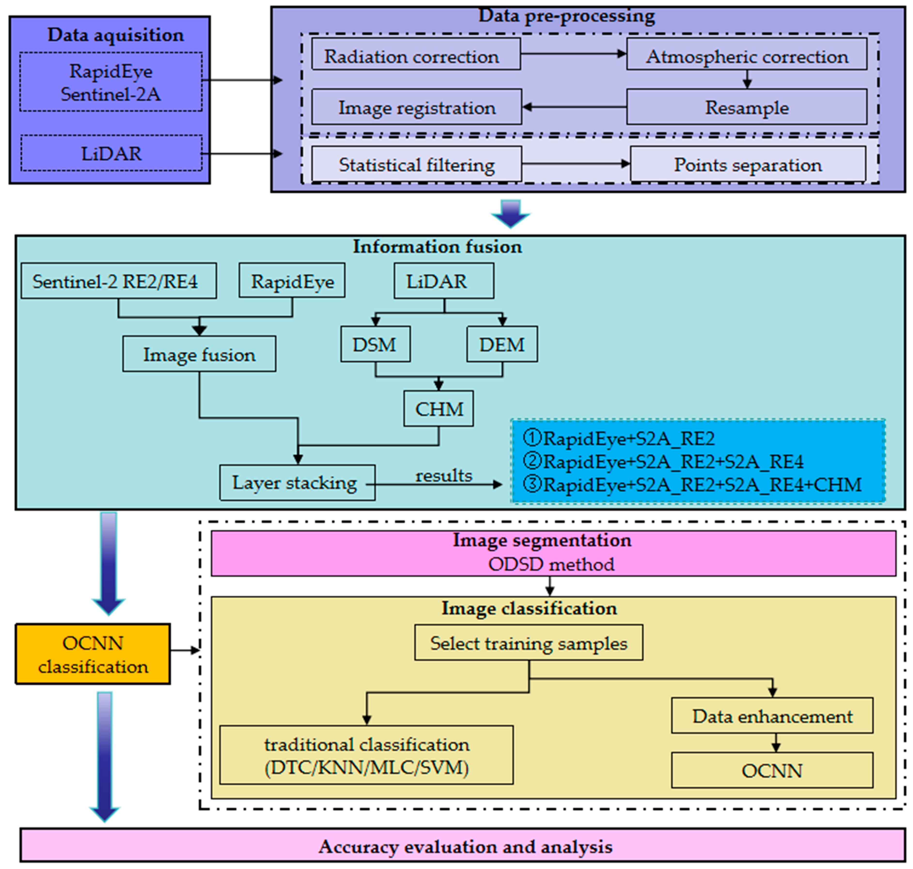
3. Methods

First, in order to explore the effectiveness of red edge spectral information in improving forest stand classification accuracy, the image fusion algorithm was used to utilize the 5 m RapidEye bands to increase the resolution of the 20 m resolution RE2 and RE4 bands in Sentinel-2A to 5 m, which were then sequentially integrated into the 5 m RapidEye image to carry out classification experiments. Afterwards, due to differences in the growth height of different stand species, combining canopy height information into the aforementioned multispectral data further improved classification accuracy. Then, image segmentation algorithms were employed to divide the data source into multiple objects, facilitating classification. Finally, four control experiments were conducted based on various data sources. In each experiment, we compared traditional object-oriented classification methods, including decision tree classification (DTC), K-nearest neighbor (KNN), maximum likelihood classification (MLC), and support vector machine (SVM), with object-oriented convolutional neural network (OCNN) classification models, such as AlexNet, LeNet, and ResNet_18 (Figure 3).

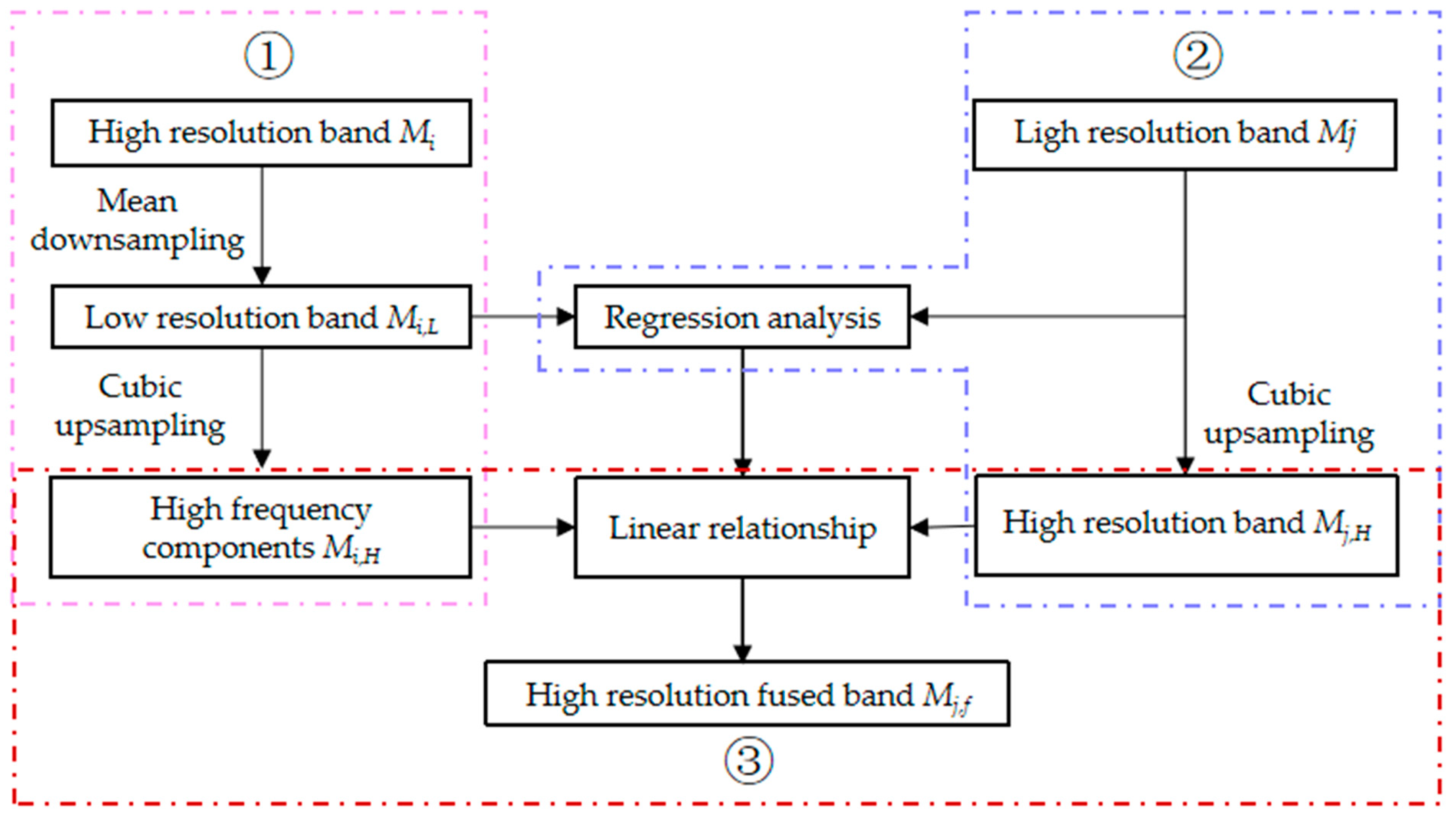
3.1. Image Fusion

The purpose of this study on image fusion is to increase the spatial resolution of Sentinel-2A images in the RE2 and red RE4 bands from 20 m to 5 m, and then combine them with RapidEye sequentially to improve the spectral information of RapidEye images, verifying the effectiveness of the red edge band in improving the accuracy of forest stand classification. General image fusion uses high-resolution panchromatic bands to fuse low resolution multispectral bands. Classical algorithms such as intensity hue saturation (IHS), principal component analysis (PCA), wavelet transform (WT) and Gram–Schmidt (GS) were available. However, in the absence of panchromatic images, conventional methods cannot be directly applied for fusion. Unlike general fusion, this study used a fusion between different data sources, and commonly used fusion methods were not applicable. Jing et al. [46] proposed an image fusion algorithm called multivariate analysis (MV) for thermal infrared images based on the idea of multi-scale analysis. This fusion algorithm combines high-frequency information from high-resolution bands with low-frequency information from low-resolution bands to obtain fused images, and it can be applied to the integration of diverse data sources. Ge [47] applied it to the fields of near-infrared visible light and shortwave infrared light, using the 10 m resolution band of Sentinel-2A to fuse the 20 m and 60 m bands, improving the spatial resolution of Sentinel-2A images, and studied the application prospects of fused images in geological and mineral information extraction. The specific principle of the MV algorithm is as follows, and the computation flow is illustrated in Figure 4:

(1)

Using the average downsample method, reduce the high-resolution bands M_i (i = 1, …, n) to the same pixel size as the low resolution band to obtain the low-frequency components M_i,L. Then, use cubic convolution to sample M_i,L back to the original pixel size and calculate their spatial detail information M_i,h:

$$M_{i,h}=M_i-M_{i,L}$$

(1)

(2)

Establish a linear relationship f between the low resolution band M_j (j = 1, …, m) to be fused and the low-frequency components M_i,L of n high-resolution bands and obtain n correlation coefficients a_i (i = 1…, n):

$$M_j={\displaystyle \sum _{i=1}^n{a}_i{M}_{i,L}+b}$$

(2)

Of these, a_i and b are linear regression coefficients determined by the least-squares method.

(3)

Conduct three convolutional operations to upsample M_j to the pixel size of M_i, denoted as M_j,h, and compute the fusion band M_j,f:

$$M_{j,f}=M_{j,h}+{\displaystyle \sum _{i=1}^n{a}_i{M}_{i,h}}$$

(3)

Multi-source remote sensing data fusion presents a certain level of complexity and difficulty. Data generated by different sensors differ in format, resolution, data quality, and spatial reference systems. Multi-source data require preprocessing, registration, and fusion. The demands on algorithms are high, making data fusion extremely challenging. Although the MV fusion method used in this study has solved these problems to some extent, it still involves uncertainty. Therefore, it was necessary to strengthen the control and evaluation of data quality to enhance data reliability.

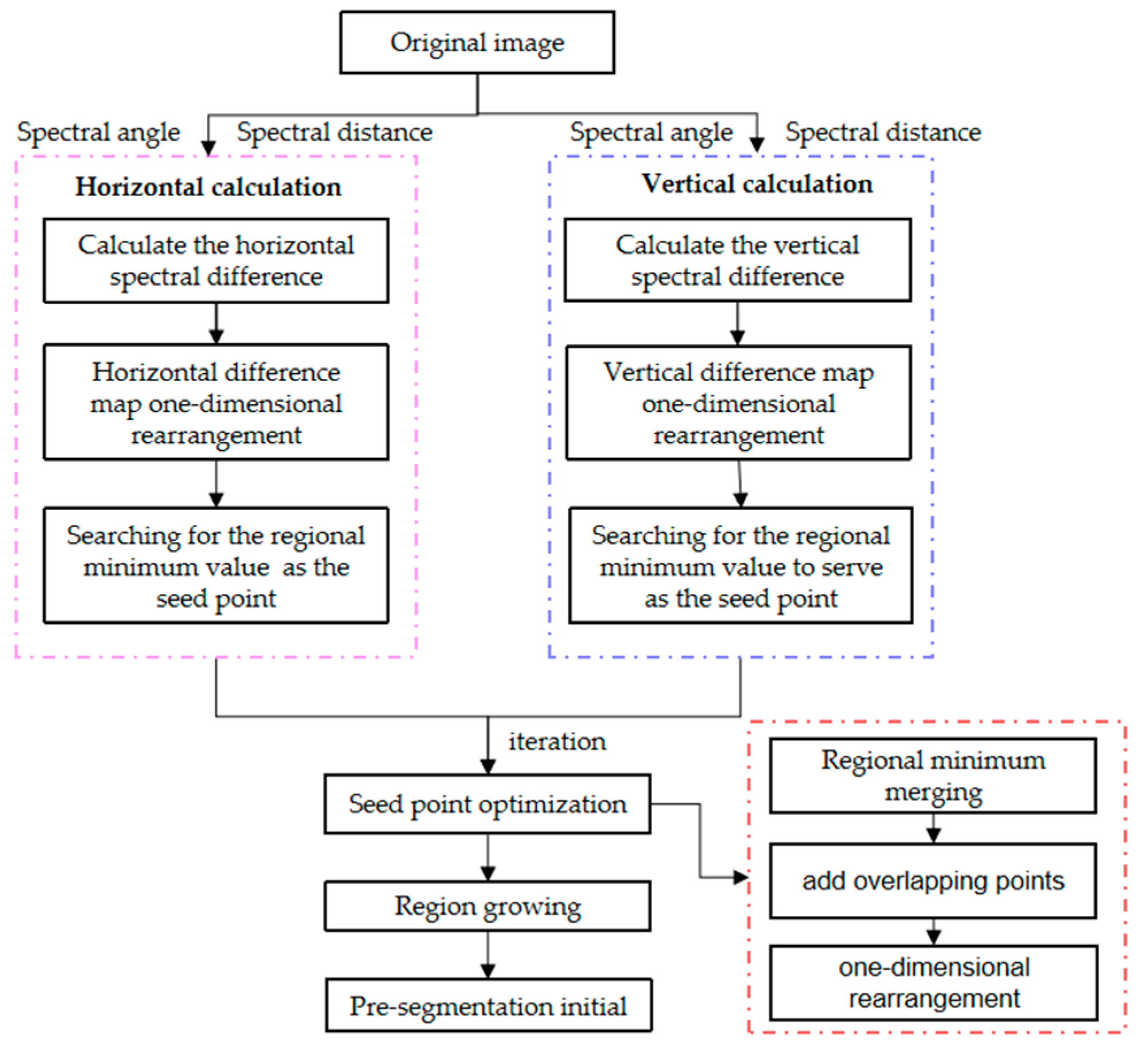
3.2. Image Segmentation

Image segmentation is a key step in object-oriented classification. The segmentation method used in this article is the one-dimensional spectral difference (ODSD) method for selecting seed points based on one-dimensional spectral differences, proposed by Li [48]. This method was proposed to address the problems of excessive number of seed points, low efficiency, and insufficient seed points for terrain details in existing seed point selection methods; compared with other methods, it can achieve maximum heterogeneity between image blocks and minimum homogeneity within each image block to a greater extent. The key steps of the algorithm are seed point selection and seed point optimization. Because the selected seed points must possess strong representativeness and exhibit high similarity with neighboring pixels, the selection of seed points employs spectral angle and spectral distance as the criteria for calculating spectral differences between pixels.

(1)

Spectral angle (SA) considers spectral data as vectors in multidimensional space, and the angle between vector pixels and their adjacent vector pixels is the spectral angle between two pixels. The size of the spectral angle between adjacent pixels can measure the spectral difference between pixels. The spectral angle between vector pixels a and b is as follows:

$$SA(a,b)={\cos }^{-1}(\frac{a\cdot b}{\left|a\right|\cdot \left|b\right|})$$

(4)

In the formula, | | represents the length of the calculated vector pixel; a·b is the product of the quantity of vector pixels a and b. The value of SA falls within [0, 1]. The smaller the SA, the smaller the angle between vectors, indicating a higher spectral similarity between pixels. Conversely, the larger the SA, the greater the angle between vectors, and the lower the spectral similarity between pixels.

(2)

Spectral distance (dist) refers to treating spectral data as vectors in a multidimensional space, and the distance between vector pixels and their adjacent pixels is the spectral distance between two pixels. Spectral distance is a measure of the brightness value of a pixel, and its calculation formula is as follows:

$$dist(a,b)=|a-b|$$

(5)

In the formula, |a − b| represents the Euclidean distance between the pixel vectors a and b. The smaller the value of dist, the closer the distance between vectors, and the closer the spectral brightness values between pixels are.

(3)

Combining SA and dist indicators defines the spectral difference dif between pixels:

$$dif(a,b)=\frac{dist(a,b)}{dist(a)}\cdot SA(a,b) dist(a,b)=|a-b|$$

(6)

In the formula, dist (a, b) represents the spectral distance between vectors a and b, dist (a) represents the spectral length of vector pixel a, and the value of dif (a, b) falls within [0, 1].

First, calculate the difference between pixel p(i, j) and its adjacent pixels horizontally to the right p (i, j + 1) or vertically to the right p (i + 1, j) in the row and column directions of the image. Add up the difference values of k bands for each pixel and calculate the square root as the difference between the pixel and its adjacent pixels. Record the difference in the spectral difference map dif_H(i,j) and dif V (i, j); next, dif_H(i, j) and dif V (i, j) are split along the row and column directions and rearranged into a 1-dimensional matrix respectively. Conduct an imHmin transformation in the 1-dimensional direction, remove shallow minima, and then search for local minima as the initial seed points. Then merge the local minima in both directions and find the common positions of the horizontal and vertical seed points on the original horizontal and vertical seed maps. Finally, conduct a 1-dimensional rearrangement of the horizontal and vertical seed point graphs with added common points; the computation flow is illustrated in Figure 5.

Owing to the complexity and diversity of high-resolution images, image segmentation is challenging due to the need for multi-scale expression and multi-source feature representation. The ODSD segmentation algorithm, employed in this study, was refined to overcome the challenges posed by existing seed point selection methods—namely, the excessive number of seed points, suboptimal selection efficiency, and insufficient selection in finer target details. However, the outcomes still exhibited inherent jagged edges and objects that were either under- or over-segmented. By continuously adjusting parameters, one could opt for the most optimal segmentation result.

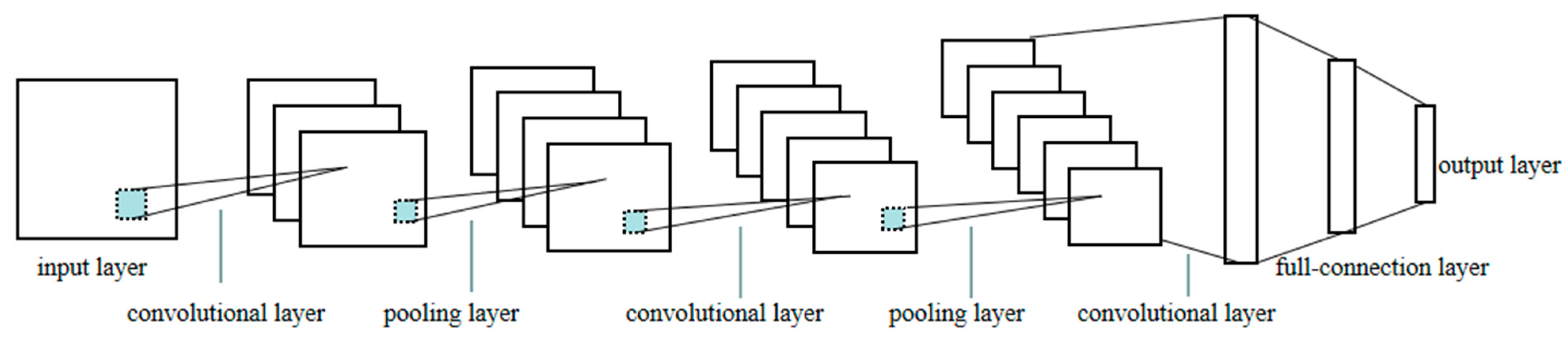
3.3. CNN Structure

CNN usually consists of five parts: input layer, convolutional layer, pooling layer, fully connected layer, and output layer. The basic network structure is shown in Figure 6. The input layer is a matrix of M × N × C, where M and N represent the length and width of the matrix, and C represents the number of channels for the input matrix. Each convolutional layer contains several convolution kernels; the size and movement step of each kernel can be adjusted as needed, but the depth must align with the number of channels in the input layer. Typically, the number of convolutional kernels increases as the network depth deepens with the aim of progressively extracting deep features of image objects. The pooling layer is typically positioned after the convolutional layer via two primary methods: average pooling and maximum pooling. The purpose is to reduce feature dimensionality, condense data and parameter counts, minimize overfitting, and enhance the model’s fault tolerance. The fully connected layer plays the role of a classifier within the neural network, integrating highly abstracted features from multiple convolutions and mapping the learned ‘distributed feature representations’ to the sample label space. The structure and operation of the output layer are consistent with those of traditional feedforward neural networks, using logic functions or normalized exponential functions to output classification labels.

The challenge faced regarding the CNN employed in this study was to enhance the model’s generalization capabilities. Not all models can be applied to a completely new dataset. This can be achieved through more diverse training data, regularization techniques, and trying multiple networks to find the best model suitable for forest classification. The limitation of CNN is that it is often seen as a ‘black box’, and it is difficult to explain its internal working principles.

3.4. Experimental Design

According to the Technical Regulations for Continuous Inventory of Forest Resources in China (State Forestry Administration, 2014), a classification system is established based on the land cover status of the study area and data collected from field ground points. Due to the research’s focus on distinguishing tree species in forest stands, water bodies, construction land, bare land, and other forest lands (felling blank, unforested land) in the study area were collectively classified as ‘others’. Forest stands were divided into: star anise, eucalyptus, Chinese fir, pine trees, and other broad-leaved trees (due to the presence of multiple rare tree species in the study area, but as they were limited by sampling points, they were collectively classified as ‘other broad-leaved trees’).

As shown in

Table 2. Experimental design.

Data Source	Traditional Object-Oriented	Object-Oriented_CNN
RapidEye	DTC KNN MLC SVM	AlexNet LeNet ResNet_18
RapidEye + S2A Red-egde2 (RapidEye + RE2)
RapidEye + S2A Red-egde2 + S2A Red-egde4 (RapidEye + RE2 + RE4)
RapidEye + S2A Red-egde2 + S2A Red-egde4 + CHM (RapidEye + RE2 + RE4 + CHM)

, to illustrate the influence of incorporating red edge band and forest height information on classification outcomes, the study evaluated the forest classification results of four data sources, including RapidEye images, RapidEye images combined with the fused RE2 (RapidEye + RE2), RapidEye images combined with the fused RE2 and RE4 (RapidEye + RE2 + RE4), RapidEye image combined with the fused RE2, RE4 and CHM (RapidEye + RE2 + RE4 + CHM). Based on the above data, these images were compared with the traditional object-oriented classification methods DTC, KNN, MLC, and SVM, and OCNN models, namely AlexNet, LeNet, and ResNet_18. Traditional object-oriented classification methods necessitate the manual selection of training features. Three spectral features (pixel mean, variance and brightness) plus six texture features (compactness, energy, moment of inertia, inverse moment difference, entropy, and correlation) were selected for training. Convolutional neural networks only require the input of various sample types, allowing the network to automatically learn the features of these samples. Parameter settings for the CNN are provided in

Table 3. CNN parameter settings.

Input Image Size	Train Epoch	Batch_Size	Classifier	Monitor Quantity	Save Best Model
64	200	16	Softmax	Val_acc	True

.

3.5. Training Samples Selection and CNN Sample Set Construction

Samples of star anise, eucalyptus, Chinese fir, pine trees, and ‘other broad-leaved’ species were selected from field-collected sample points in conjunction with segmentation outcomes. Training samples for ‘other’ were selected through visual interpretation combined with segmentation results, ensuring that each segmentation object encompassed only a single sample point. A total of 330 samples were ultimately selected, consisting of 58 star anise samples, 62 eucalyptus samples, 65 Chinese fir samples, 43 pine tree samples, 42 ‘other broad-leaved’ samples, and 60 ‘other’ samples. These samples were utilized as training samples for traditional object-oriented classification.

In convolutional neural networks, to enhance data volume, enrich data diversity, improve model generalization, and mitigate overfitting, data augmentation is employed to expand the sample library. Taking 330 sample points as the initial sample set, each sample underwent rotations of 45°, 90°, 135°, 180°, 225°, 270°, 315°, as well as up-and-down and left-and-right flips. Additionally, Gaussian noise was introduced to the original image. This expansion effectively increased the sample size by 11 times, resulting in a total of 3630 samples that were fed into the convolutional neural network for training.

4. Results

4.1. Image Fusion Results

Among various classic image fusion algorithms, GS fusion can achieve the fusion of multiple high-resolution bands to a single low resolution band, and the fusion effect is relatively stable. Therefore, a comparative analysis was conducted between the GS fusion and the MV fusion algorithms. Using the MV and GS fusion algorithms, the RE2 and RE4 bands of Sentinel-2A images with a resolution of 20 m were fused using a 5 m RapidEye image. The spatial resolution of the two vegetation red edges was improved to 5 m, and the fusion results of RE2 are shown in Figure 7.

Upon visual comparison, it is evident that both fusion methods enhanced the clarity of the RE2 band. GS fusion excelled in non-forest areas such as roads, water bodies, and buildings, while MV fusion outperformed GS fusion in forest distribution. Furthermore, upon zooming in locally, the forest features in the MV-merged image stood out more, effectively preserving the information of the original RE2 band. The spectral information from the low-resolution band was effectively combined with the texture information from RapidEye. Conversely, the RE2 noise phenomenon after GS fusion was more pronounced, and the forest features were not well preserved.

This study used six evaluation metrics for image fusion to quantitatively analyze the fusion results, including mean (M), deviation (STD), entropy (EN), average gradient (AG), spatial frequency (SF), and cross entropy (CEN).

Table 4. Comparison of Sentinel-2 RE2 band fusion quality evaluation metrics. M: The mean represents the brightness of an image, with optimal image quality maintaining a suitable range of mean values, avoiding excessively high or low values. STD: Measures the dispersion of information within an image; a larger standard deviation indicates a greater amount of information. EN: An indicator of the richness of image information, with a higher value indicating greater information content. AG: Reflects the fineness of local details in an image, measuring how distinct the details appear. SF: Measures the overall activity level of an image in the spatial domain, reflecting the rate of grayscale value changes. CEN: the dissimilarity between corresponding positions in the fused and source images.

Method	Evaluation Indicators
	M	STD	EN	AG	SF	CEN
MV	144.59	65.64	7.03	14.01	28.75	0.07
GS	131.91	50.51	6.85	17.61	37.32	0.28

indicates that the image quality of both fusion outcomes remained within a suitable range. Although the visual clarity of the MV algorithm’s fusion outcome was slightly less sharp, it exhibited greater information richness and overall image quality. Given that the primary objective of this study is to preserve RE2 spectral information to compensate for RapidEye images’ spectral deficiencies, a comprehensive analysis revealed that the MV fusion results are better than GS fusion results in enhancing the spatial detail information and spectral information fidelity of RE2 images, which can be used for subsequent classification.

4.2. Image Segmentation Results

The classification process comprises segmentation and classification, both of which influence the final classification accuracy. To ensure the final classification results were not influenced by the segmentation results, this study adopted a method of controlling variables and only segmented the 5 m RapidEye image. The segmented vector patches were used to segment all subsequent data sources for the following classification, thereby ensuring the classification results were solely influenced by the classification method. The segmentation parameter settings are presented in

Table 5. Segmentation parameter settings.

Data Source	Layer Weight	Scale Rang	Scale Step Size	Color Indices	Tightness Indices
5 m RapidEye	1	20–100	10	0.9	0.5

.

By adjusting the segmentation scale, multiple segmentation results were obtained. After visually observing the segmentation results, it could be found that due to the fact that the study area was predominantly covered by forest land, the spectral similarity among objects was high and non-forest land could be distinctly segmented from the forest, yet for regions with forest land, the segmentation boundary failed to achieve a smooth transition, resulting in jagged or irregular shapes. Upon a detailed analysis of the segmentation results, taking the area within the blue frame in the Figure 8 as a reference, this area should have belonged to two types of forest stands. When the segmentation scale was 20 and 30, the segmentation objects were relatively fragmented, and there was obvious over-segmentation, which indicates that the segmentation scale was undersize However, when the segmentation scale was greater than 40, the area within the blue frame was divided into one object, which was under-segmented. When the segmentation scale was 40, the boundaries of each forest stand could be well distinguished, and there was less occurrence of two or more forest types in one object. Therefore, a segmentation result with a segmentation scale of 40 was ultimately chosen as the optimal segmentation result for implementing subsequent classification.

4.3. Classification Results

This study adopted a random sampling method to collect verification points. A total of 419 validation points were randomly collected in the area where training samples were excluded, and then the confusion matrix was calculated to obtain accuracy evaluation indicators, consisting of user’s accuracy (UA), producer’s accuracy (PA), overall accuracy (OA), and kappa coefficient. The OA of traditional classification methods and OCNN models are shown in

Table 6. Overall classification accuracy.

Methods OA (%) Data Source	RapidEye	RapidEye +RE2	RapidEye +RE2 +RE4	RapidEye +RE2 +RE4 +CHM
DTC	52.27	60.62	61.10	62.29
KNN	55.61	58.23	59.43	60.86
MLC	73.03	74.70	75.66	80.91
SVM	76.85	77.80	78.52	81.15
AlexNet	74.22	75.18	79.24	79.95
LeNet	78.28	79.47	81.62	84.49
ResNet_18	81.38	83.29	84.49	85.68

.

In terms of classification methods, the accuracy of DTC and KNN classification methods in traditional classification methods was relatively low, both below 61%; MLC and SVM had relatively high classification accuracy, both above 70%. Among them, SVM had the best classification performance, with classification accuracy of 76.85%, 77.80%, 78.52%, and 81.15%, respectively, for the four data sources. In OCNN models, the ResNet_18 stood out with its superiority among various network structures, with significantly higher classification accuracy than SVM; the classification accuracy of the four data sources was 81.38%, 83.29%, 84.49%, and 85.68%, respectively. The classification results of SVM and ResNet_18 are illustrated in Figure 9. SVM’s classification results were relatively fragmented, with categories intermingled, not forming distinct stands. while ResNet_18’s classification results exhibited clearer and more uniform stand boundaries, reducing the occurrence of mixed stands.

From the perspective of classification data sources, both traditional classification methods and OCNN continuously improved classification accuracy by adding RE2 and RE4′s spectral information of Sentinel-2, as well as tree height information provided by LiDAR, on top of RapidEye’s original four spectral bands. Among them, the DTC method exhibited the most pronounced effect when incorporating spectral and height information, resulting in an accuracy improvement of 10.02%.

5. Discussion

To evaluate the final classification performance,

Table 7. ResNet_18_RapidEye + RE2 + RE4 + CHM classification confusion matrix.

	Actual Number of Sample Points
Category	Others	Octagon	Eucalyptus	Cedar	Pine	Other Broad-Leaved	Total
others	72	4	2	0	5	2	85
Octagon	2	51	0	0	1	0	54
eucalyptus	1	2	87	1	0	0	91
Cedar	1	1	1	69	2	6	80
pine	3	2	2	7	35	8	57
Other broad-leaved	0	0	2	4	1	45	52
total	79	60	94	81	44	61	419

presents ResNet_18_ RapidEye + RE2 + RE4 + CHM confusion matrix, where the sum of each row represents the number of samples identified as the category, and the sum of each column represents the actual number of samples in the category. It is evident that the ‘Other’ category and the pine tree category have a higher number of discriminative sample points than the actual sample points, implying that some samples not belonging to these categories have been misclassified by the network. The remaining four categories all have actual sample points higher than the discriminative sample points, suggesting that samples that should have belonged to these categories were mistakenly classified as the ‘Other’ category. Analyze the reasons of the inaccuracies, the ‘other’ category includes felling blank and unforested land, displaying spectral characteristics akin to those of forest lands, potentially leading to spectral confusion and misclassifications. Chinese fir and pine both belong to coniferous forests and have similarities in texture structure. The area proportion of pine trees and other broad-leaved trees in the study area is relatively minor, and the number of training samples that could be collected is also limited. Therefore, feature learning may not be exhaustive enough, resulting in a heightened error rate in distinguishing these two categories. The accuracy of training samples is also very important. Although we have tried to select pure forests of various categories when selecting training samples, it is inevitable that a small number of non-pure forests will be selected, which may also affect classification accuracy.

There are two reasons why OCNN has high classification accuracy. One reason is the combination of CNN and object-oriented methods utilizes the peripheral information of forest objects and bounding rectangles and extracts deep abstract information through a large number of convolutional layers, while traditional classification only uses a few manually selected statistical information. Another reason is that CNN increases a large number of learning samples through data augmentation, while traditional classification only selects a few hundred samples. This result demonstrates the effectiveness of OCNN in forest classification and can to some extent improve the accuracy of forest classification. ResNet_18 achieves high classification accuracy among the three classic CNN networks due to its inherent advantages: its unique residual unit addresses the issue of gradient vanishing as the network depth increases, significantly simplifying the model optimization process, cause the magnitude of the training error to be inversely proportional to the number of network layers, thereby achieving satisfactory testing performance.

Correct forest stand species identification is essential for forest inventories, as it is the basis for forest biomass calculations, carbon storage assessment, habitat, ecosystem and socio-economic sustainable development. Our method will complement other approaches to identify stand species based on remote sensing, will help to increase overall accuracy, and thus, will support the more efficient creation of forest inventories. This assumption is based on the future possibility of achieving high-precision automatic or semi-automated classification processes. Our research aims to explore this process.

While the creation of a multi-source remote sensing dataset for forest stands has validated the efficacy of the OCNN and ResNet_18 model, our study has some limitations. Firstly, some forest types have relatively few training samples and are prone to becoming stuck in local optima, which will affect the feature learning process of the category and thus affect classification accuracy. Secondly, Although the study area of this experiment is already a complex forest type, the universality of the model under different geographical, climatic or ecological conditions still needs further verification. Thirdly, its learning process can be seen as a ‘black box’. Although it has strong adaptability to data, this leads to weak interpretability in the operation process, making it difficult to grasp the key parameters in the feature learning process. Future research should focus on increasing the size and diversity of the training data set to improve the accuracy and robustness of the machine learning models. Moreover, there is a need to strengthen the explainability of automatic quantitative visual representation, and explore the feature learning process of deep neural networks through automation, verify the universality of the model under more diverse geographical, climatic, or ecological conditions.

6. Conclusions

Addressing the prevalent issues in forest stand classification research, namely the underutilization of red edge band information as well as the issues of strong human dependence and incomplete information extraction in traditional classification methods. The study mainly uses RapidEye and Sentinel-2A images which containing the red edge bands as the primary data source. By incorporating the fused red edge 2 and red edge 4 bands of Sentinel-2A images into RapidEye images, the potential of the red edge band in enhancing forest classification accuracy is confirmed. Furthermore, the canopy height information derived from LiDAR point clouds is integrated to further improve classification accuracy. The classification method integrates object-oriented and convolutional neural networks (OCNN) to circumvent the limitations of incomplete information extraction stemming from manual feature selection. This method is then compared to traditional object-oriented classification methods. Upon analyzing the research outcomes, the following conclusions are drawn:

(1)

With the integration of the red edge band information into RapidEye, the accuracy of forest stand classification improves continuously. Prove that the fusion design proposed in this experiment can effectively increase the spectral information used for classification and improve the application range of Sentinel-2, which is highly significant for forest classification.

(2)

By integrating object-oriented techniques with convolutional neural networks (OCNN), a pathway is established for constructing deep learning sample libraries. This approach not only prevents the emergence of ‘salt-and-pepper noise’ but also ensuring the integrity and homogeneity of the stands.

(3)

The canopy height information derived from LiDAR point clouds can, to a certain extent, enhance the precision of forest stand classification.

(4)

Comparing traditional object-oriented classification with OCNN classification methods, it is found that the classification accuracy of ResNet_18 is the highest. For the classification results of four data sources using ResNet_18, there is an enhancement of 4.53%, 5.49%, 5.97%, and 4.53% than SVM method, which holds the highest classification accuracy among traditional methods. The OCNN classification method has been demonstrated to be effective in identifying forest stands, offering a viable approach for the precise identification of forest tree species.

References

- Ye, M.; Zhao, Y.; Im, J.; Zhao, Y.; Zhen, Z. A deep-learning-based tree species classification for natural secondary forests using unmanned aerial vehicle hyperspectral images and LiDAR, Ecological Indicators. Remote Sens. 2024, 159, 111608. [Google Scholar]
- Gong, Y.; Li, X.; Du, H.; Zhou, G.; Mao, F.; Zhou, L.; Zhang, B.; Xuan, J.; Zhu, D. Tree Species Classifications of Urban Forests Using UAV-LiDAR Intensity Frequency Data. Remote Sens. 2023, 15, 110. [Google Scholar] [CrossRef]
- Chen, Y.; Zhao, S.; Xie, Z.; Lu, D.; Chen, E. Mapping multiple tree species classes using a hierarchical procedure with optimized node variables and thresholds based on high spatial resolution satellite data. Remote Sens. 2020, 57, 526–542. [Google Scholar] [CrossRef]
- Shi, W.; Wang, S.; Yue, H.; Wang, D.; Ye, H.; Sun, L.; Sun, J.; Liu, J.; Deng, Z.; Rao, Y.; et al. Identifying Tree Species in a Warm-Temperate Deciduous Forest by Combining Multi-Rotor and Fixed-Wing Unmanned Aerial Vehicles. Drones 2023, 7, 353. [Google Scholar] [CrossRef]
- Mielczarek, D.; Sikorski, P.; Archiciński, P.; Ciężkowski, W.; Zaniewska, E.; Chormański, J. The Use of an Airborne Laser Scanner for Rapid Identification of Invasive Tree Species Acer negundo in Riparian Forests. Remote Sens. 2023, 15, 212. [Google Scholar] [CrossRef]
- Jia, W.; Pang, Y. Tree species classification in an extensive forest area using airborne hyperspectral data under varying light conditions. J. For. Res. 2023, 34, 1359–1377. [Google Scholar] [CrossRef]
- Eisfelder, C.; Kraus, T.; Bock, M.; Werner, M.; Buchroithner, M.F.; Strunz, G. Towards automated forest-type mapping—A service within GSE forest monitoring based on SPOT-5 and IKONOS data. Int. J. Remote Sens. 2009, 30, 5015–5038. [Google Scholar] [CrossRef]
- Liu, Y.; Gong, W.; Hu, X.; Gong, J. Forest type identification with random forest using sentinel-1a, sentinel-2a, multi-temporal landsat-8 and dem data. Remote Sens. 2018, 10, 946. [Google Scholar] [CrossRef]
- Xu, H.; Pan, P.; Yang, W.; Ouyang, X.; Ning, J.; Shao, J.; Li, Q. Classification and Accuracy Evaluation of Forest Resources Based on Multi-source Remote Sensing Images. Acta Agric. Univ. Jiangxiensis 2019, 41, 751–760. [Google Scholar]
- Lin, H.; Liu, X.; Han, Z.; Cui, H.; Dian, Y. Identification of Tree Species in Forest Communities at Different Altitudes Based on Multi-Source Aerial Remote Sensing Data. Appl. Sci. 2023, 13, 4911. [Google Scholar] [CrossRef]
- Machala, M. Forest mapping through object-based image analysis of multispectral and lidar aerial data. Eur. J. Remote Sens. 2014, 47, 117–131. [Google Scholar] [CrossRef]
- Dechesne, C.; Mallet, C.; Le Bris, A.; Gouet, V.; Hervieu, A. Forest stand segmentation using airborne lidar data and very high resolution multispectral imagery. ISPRS—Int. Arch. Photogramm. Remote Sens. Spat. Inf. Sci. 2016, XLI-B3, 207–214. [Google Scholar] [CrossRef]
- Xie, Z.; Chen, Y.; Lu, D.; Li, G.; Chen, E. Classification of land cover, forest, and tree species classes with ziyuan-3 multispectral and stereo data. Remote Sens. 2019, 11, 164. [Google Scholar] [CrossRef]
- Dalponte, M.; Bruzzone, L.; Gianelle, D. Tree species classification in the southern alps based on the fusion of very high geometrical resolution multispectral/hyperspectral images and lidar data. Remote Sens. Environ. 2012, 123, 258–270. [Google Scholar] [CrossRef]
- Ghosh, A.; Fassnacht, F.E.; Joshi, P.K.; Koch, B. A framework for mapping tree species combining hyperspectral and lidar data: Role of selected classifiers and sensor across three spatial scales. Int. J. Appl. Earth Obs. 2014, 26, 49–63. [Google Scholar] [CrossRef]
- Yifang, S.; Skidmore, A.K.; Tiejun, W.; Stefanie, H.; Uta, H.; Nicole, P.; Zhu, X.; Marco, H. Tree species classification using plant functional traits from lidar and hyperspectral data. Int. J. Appl. Earth Obs. 2018, 73, 207–219. [Google Scholar]
- Akumu, C.E.; Dennis, S. Effect of the Red-Edge Band from Drone Altum Multispectral Camera in Mapping the Canopy Cover of Winter Wheat, Chickweed, and Hairy Buttercup. Drones 2023, 7, 277. [Google Scholar] [CrossRef]
- Weichelt, H.; Rosso, R.; Marx, A.; Reigber, S.; Douglass, K.; Heynen, M. The RapidEye Red-Edge Band-White Paper. Available online: https://apollomapping.com/wp-content/user_uploads/2012/07/RapidEye-Red-Edge-White-Paper.pdf (accessed on 3 November 2022).
- Cui, B.; Zhao, Q.; Huang, W.; Song, X.; Ye, H.; Zhou, X. Leaf chlorophyll content retrieval of wheat by simulated RapidEye, Sentinel-2 and EnMAP data. J. Integr. Agric. 2019, 18, 1230–1245. [Google Scholar] [CrossRef]
- Wang, X.; Lu, Z.; Yuan, Z.; Zhong, H.; Wang, G. A review of the application of optical remote sensing satellites in the red edge band. Satell. Appl. 2023, 2, 48–53. [Google Scholar]
- Sothe, C.; Almeida, C.M.d.; Liesenberg, V.; Schimalski, M.B. Evaluating Sentinel-2 and Landsat-8 Data to Map Sucessional Forest Stages in a Subtropical Forest in Southern Brazil. Remote Sens. 2017, 9, 838. [Google Scholar] [CrossRef]
- Grabska, E.; Hostert, P.; Pflugmacher, D.; Ostapowicz, K. Forest Stand Species Mapping Using the Sentinel-2 Time Series. Remote Sens. 2019, 11, 1197. [Google Scholar] [CrossRef]
- Lim, J.; Kim, K.; Kim, E.; Jin, R. Machine Learning for Tree Species Classification Using Sentinel-2 Spectral Information, Crown Texture, and Environmental Variables. Remote Sens. 2020, 12, 2049. [Google Scholar] [CrossRef]
- Yang, D.; Li, C.; Li, B. Forest Type Classification Based on Multi-temporal Sentinel-2A/B Imagery Using U-Net Model. For. Res. 2022, 35, 103–111. [Google Scholar]
- Van Deventer, H.; Cho, M.A.; Mutanga, O. Improving the classification of six evergreen subtropical tree species with multi-season data from leaf spectra simulated to worldview-2 and rapideye. Int. J. Remote Sens. 2017, 38, 4804–4830. [Google Scholar] [CrossRef]
- Adelabu, S.; Mutanga, O.; Adam, E.; Cho, M.A. Exploiting machine learning algorithms for tree species classification in a semiarid woodland using rapideye image. J. Appl. Remote Sens. 2013, 101, 073480. [Google Scholar] [CrossRef]
- Long, J.A.; Lawrence, R.L.; Greenwood, M.C.; Marshall, L.; Miller, P.R. Object-oriented crop classification using multitemporal ETM+ SLC-off imagery and random forest. Gisci. Remote Sens. 2013, 50, 418–436. [Google Scholar] [CrossRef]
- Shi, J.; Li, D.; Chu, X.; Yang, J.; Shen, C. Intelligent classification of land cover types in open-pit mine area using object-oriented method and multitask learning. J. Appl. Remote Sens. 2022, 16, 038504. [Google Scholar] [CrossRef]
- Xia, T.; Ji, W.; Li, W.; Zhang, C.; Wu, W. Phenology-based decision tree classification of rice-crayfish fields from sentinel-2 imagery in Qianjiang, China. Int. J. Remote Sens. 2021, 42, 8124–8144. [Google Scholar] [CrossRef]
- Wang, P.; Ge, J.; Fang, Z.; Zhao, G.; Sun, G. Semi-automatic object—Oriented geological disaster target extraction based on high-resolution remote sensing. Mt. Res. 2018, 36, 654–659. [Google Scholar]
- Xing, Y.; Liu, P.; Xie, Y.; Gao, Y.; Yue, Z.; Lu, Z.; Li, X. Object-oriented building grading extraction method based on high resolution remote sensing images. Spacecr. Recovery Remote Sens. 2023, 44, 88–102. [Google Scholar]
- Nakada, M.; Wang, H.; Terzopoulos, D. AcFR: Active face recognition using convolutional neural networks. In Proceedings of the IEEE Conference on Computer Vision and Pattern Recognition Workshops, Honolulu, HI, USA, 21–26 July 2017; IEEE: Piscataway, NJ, USA, 2017. [Google Scholar]
- Ke, Y.H.; Quackenbush, L.J. A review of methods for automatic individual tree-crown detection and delineation from passive remote sensing. Int. J. Remote Sens. 2011, 32, 4725–4747. [Google Scholar] [CrossRef]
- Rybacki, P.; Niemann, J.; Derouiche, S.; Chetehouna, S.; Boulaares, I.; Seghir, N.M.; Diatta, J.; Osuch, A. Convolutional Neural Network (CNN) Model for the Classification of Varieties of Date Palm Fruits (Phoenix dactylifera L.). Sensors 2024, 24, 558. [Google Scholar] [CrossRef] [PubMed]
- Lemley, J.; Bazrafkan, S.; Corcoran, P. Deep Learning for Consumer Devices and Services: Pushing the limits for machine learning, artificial intelligence, and computer vision. IEEE Consum. Electron. Mag. 2017, 6, 48–56. [Google Scholar] [CrossRef]
- Garcia-Garcia, A.; Orts-Escolano, S.; Oprea, S.; Villena-Martinez, V.; Martinez-Gonzalez, P.; Garcia-Rodriguez, J. A survey on deep learning techniques for image and video semantic segmentation. Appl. Soft Comput. 2018, 70, 41–65. [Google Scholar] [CrossRef]
- Yuan, J.; Hou, X.; Xiao, Y.; Cao, D.; Guan, W.; Nie, L. Multi-criteria active deep learning for image classification. Knowl. Based Syst. 2019, 172, 86–94. [Google Scholar] [CrossRef]
- Jo, J.; Jadidi, Z. A high precision crack classification system using multi-layered image processing and deep belief learning. Struct. Infrastruct. Eng. 2020, 16, 297–305. [Google Scholar] [CrossRef]
- Zou, Q.; Ni, L.; Zhang, T.; Wang, Q. Deep Learning Based Feature Selection for Remote Sensing Scene Classification. IEEE Geosci. Remote Sens. 2015, 12, 2321–2325. [Google Scholar] [CrossRef]
- Deng, Z.; Sun, H.; Zhou, S.; Zhao, J.; Lei, L.; Zou, H. Multi-scale object detection in remote sensing imagery with convolutional neural networks. ISPRS J. Photogramm. 2018, 145, 3–22. [Google Scholar] [CrossRef]
- Muralimohanbabu, Y.; Radhika, K. Multi spectral image classification based on deep feature extraction using deep learning technique. Int. J. Bioinform. Res. Appl. 2021, 17, 250–261. [Google Scholar] [CrossRef]
- Yang, W.; Song, H.; Xu, Y. DCSRL: A change detection method for remote sensing images based on deep coupled sparse representation learning. Remote Sens. Lett. 2022, 13, 756–766. [Google Scholar] [CrossRef]
- Hakula, A.; Ruoppa, L.; Lehtomäki, M.; Yu, X.; Kukko, A.; Kaartinen, H.; Taher, J.; Matikainen, L.; Hyyppä, E.; Luoma, V.; et al. Individual tree segmentation and species classification using high-density close-range multispectral laser scanning data. ISPRS Open J. Photogramm. Remote Sens. 2023, 9, 100039. [Google Scholar] [CrossRef]
- Weinstein, B.G.; Marconi, S.; Bohlman, S.; Zare, A.; White, E. Individual Tree-Crown Detection in RGB Imagery Using Semi Supervised Deep Learning Neural Networks. Remote Sens. 2019, 11, 1309. [Google Scholar] [CrossRef]
- Xu, S.; Wang, R.; Shi, W.; Wang, X. Classification of Tree Species in Transmission Line Corridors Based on YOLO v7. Forests 2024, 15, 61. [Google Scholar] [CrossRef]
- Jing, L.; Cheng, Q. A technique based on non-linear transform and multivariate analysis to merge thermal infrared data and higher-resolution multispectral data. Int. J. Remote Sens. 2010, 31, 6459–6471. [Google Scholar] [CrossRef]
- Ge, W. Multi-Source Remote Sensing Fusion for Lithological Information Enhancement. Ph.D. Thesis, China University of Geosciences, Beijing, China, 2018. [Google Scholar]
- Li, X.; Jing, L.; Li, H.; Tang, Y.; Ge, W. Seed extraction method for seeded region growing based on one-dimensional spectral difference. J. Image Graph. 2016, 21, 1256–1264. [Google Scholar]