
Assessing the Performance of Handheld Laser Scanning for Individual Tree Mapping in an Urban Area

 , , and
Abstract
1. Introduction
2. Materials and Methods
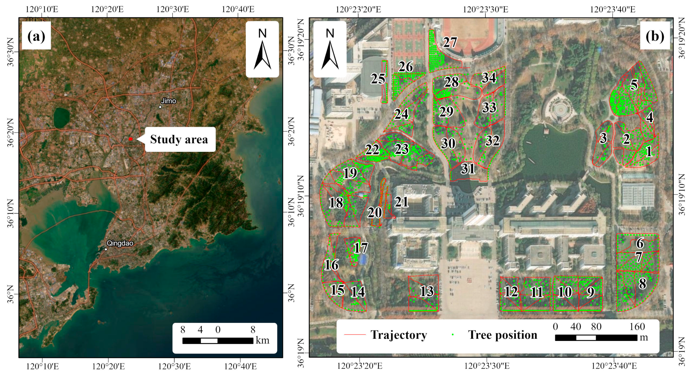
2.1. Study Area and Tree Mensuration
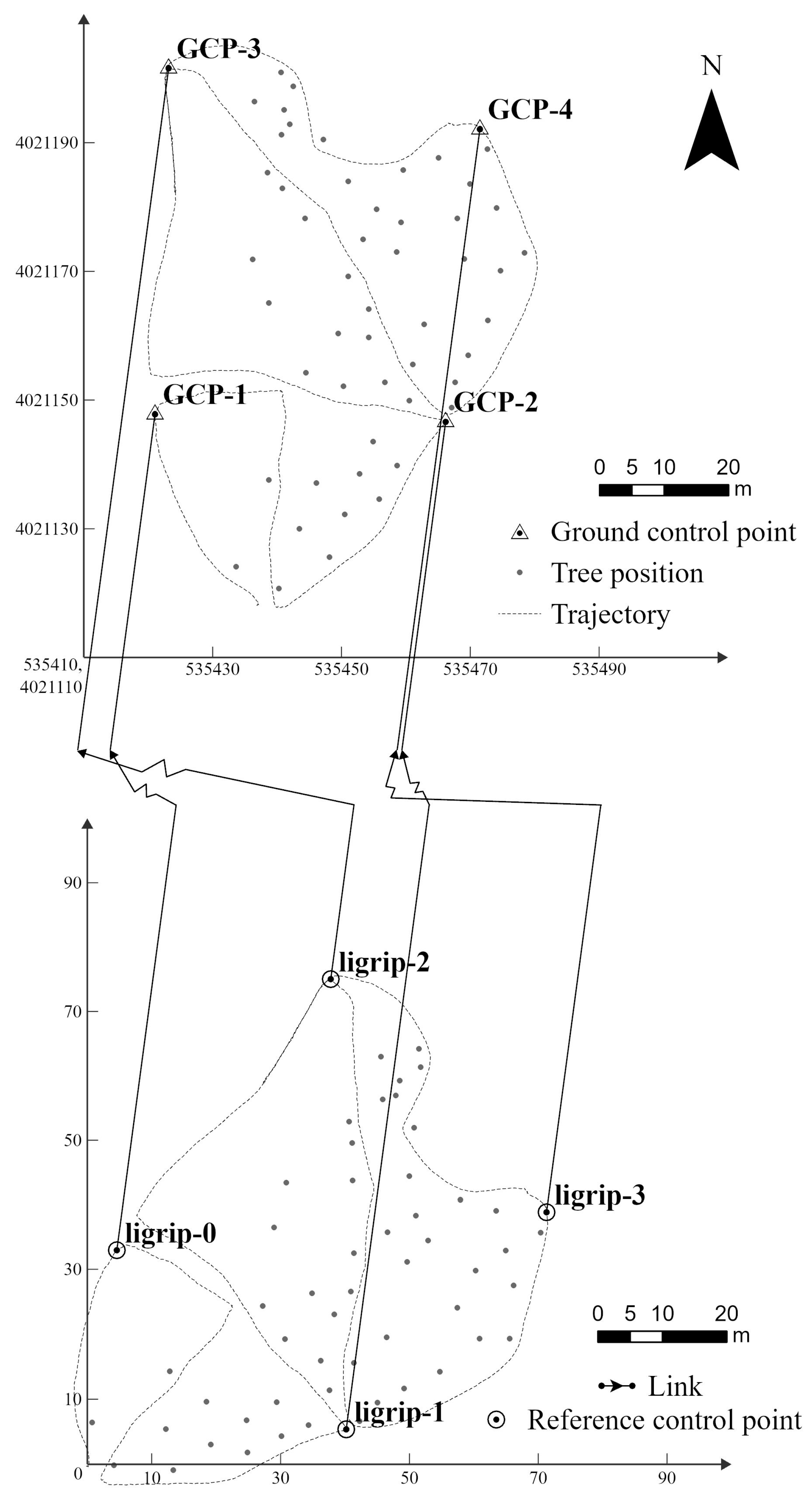
2.2. HLS Data Acquisition
2.3. Point Cloud Processing
- De-noising. Outliers resulting from multi-path errors or inaccuracies in the laser rangefinder during the measurement process were removed to enhance data quality. The default parameters of a neighborhood size 10 and a standard deviation multiplier 5 were adopted.
- Ground point classification. The Improved Progressive TIN Densification (IPTD) algorithm [11] was employed for ground point classification. This algorithm initially generates a sparse triangular network using seed points and iteratively densifies it layer by layer until all ground points are classified.
- Normalization based on ground points. The elevation value Z of the nearest ground point was subtracted from each point in the procedure of normalization to eliminate the influence of terrain undulations on the elevation values of point cloud data.
- Seed-based individual tree segmentation. Parameters such as DBH and tree height were batch-extracted using the ‘TLS Seed Point Editor’ tool under ‘TLS Forest’, based on normalized ground points. DBH was determined by cylinder fitting within the slice at a height of 1.2–1.4 m. Subsequently, each fitted DBH and tree height was inspected for anomalies, as well as potential commission or omission errors. In case of fitting errors, individual tree fitting would be carried out again. Finally, the fitted results were used as seed points for individual tree segmentation using the ‘Point Cloud Segmentation from Seed Points’ tool.
2.4. Evaluation
2.5. Statistical Analysis
3. Results
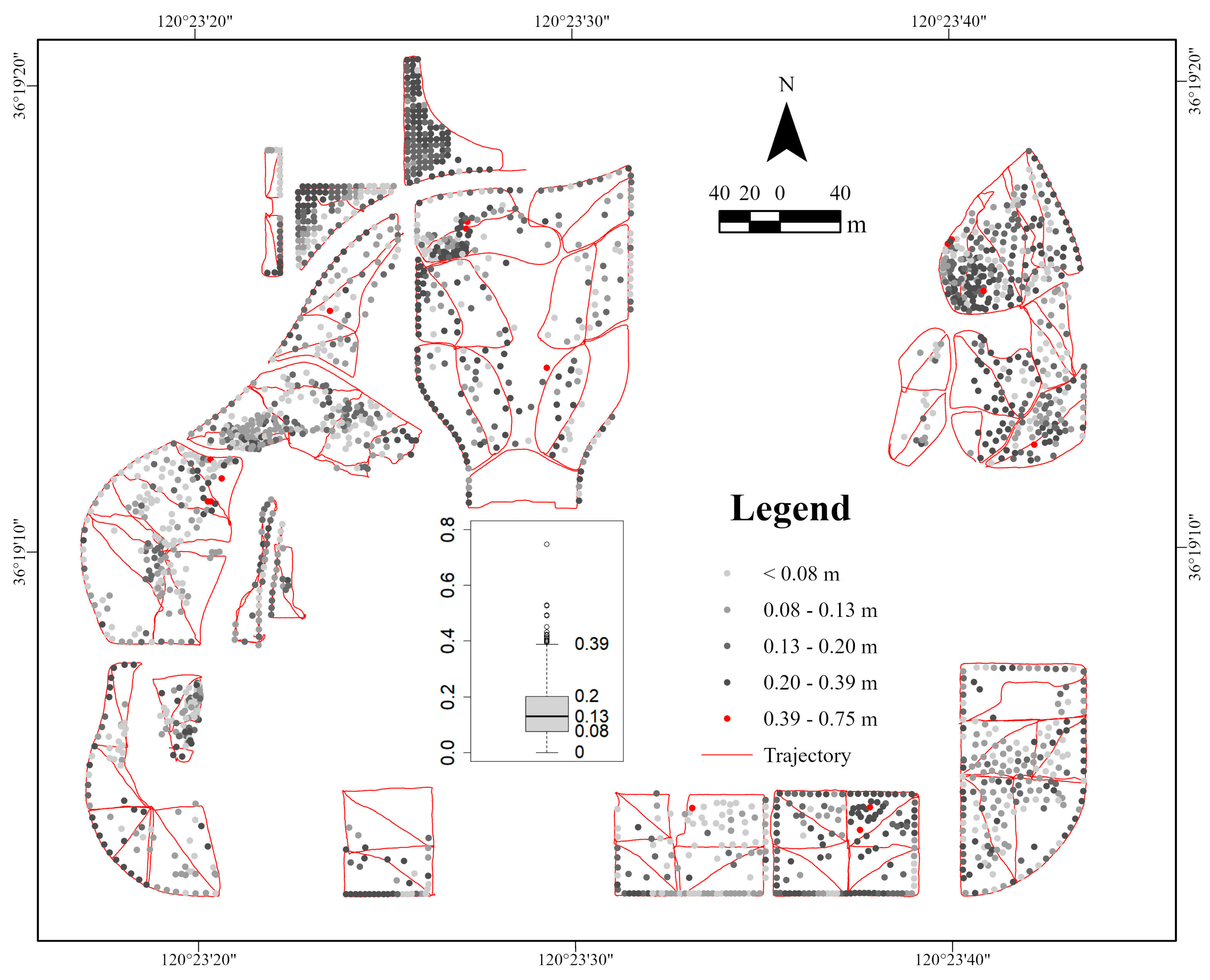
3.1. Tree Position
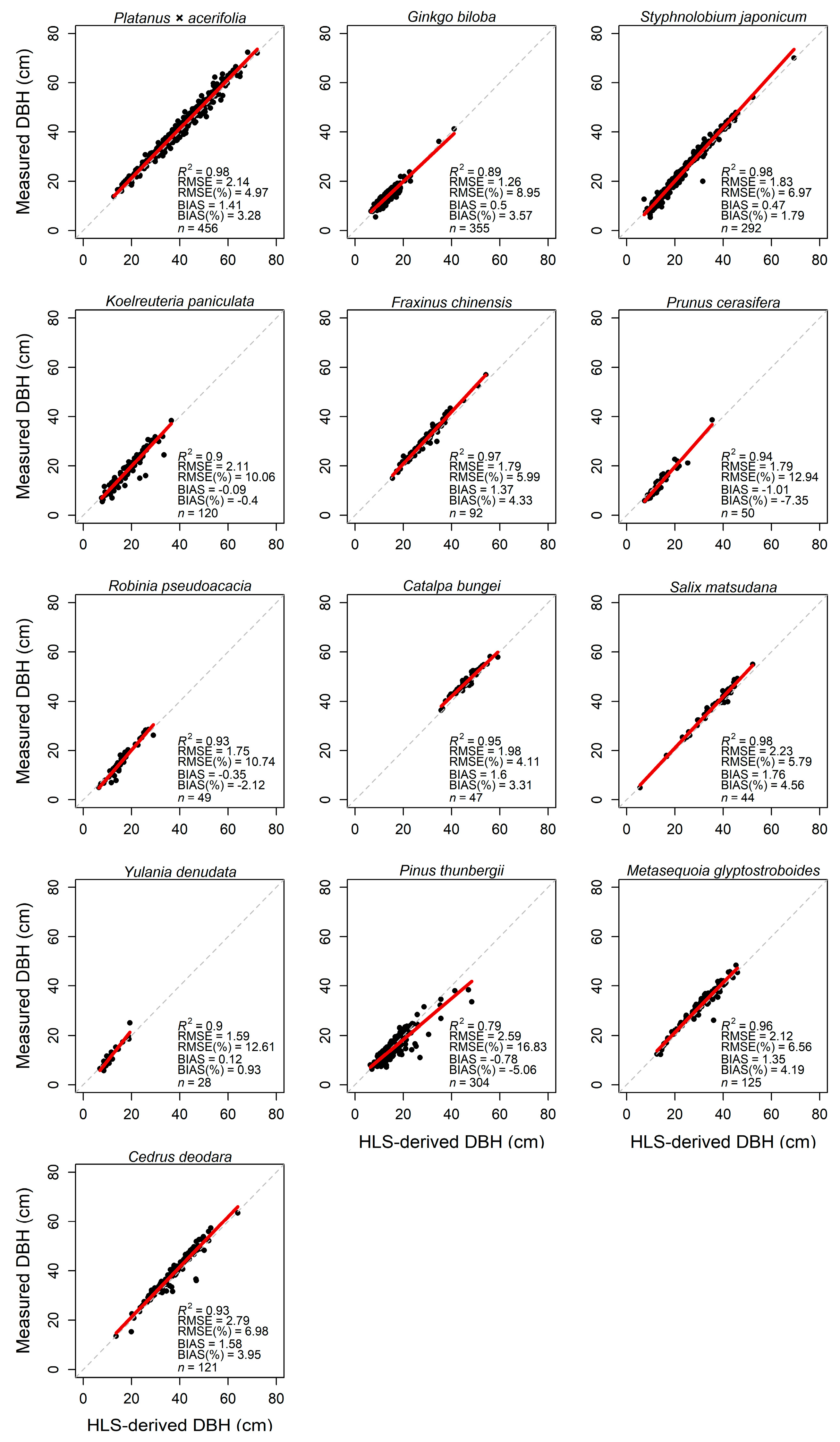
3.2. Estimation of DBH
3.3. Estimation of Tree Height
3.4. LME Results
4. Discussion
5. Conclusions
Author Contributions
Funding
Data Availability Statement
Acknowledgments
Conflicts of Interest
References
- Guo, W.; Serra-Diaz, J.; Eiserhardt, W.; Maitner, B.; Merow, C.; Violle, C.; Pound, M.; Sun, M.; Silk, F.; Blach-Overgaard, A.; et al. Climate Change and Land Use Threaten Global Hotspots of Phylogenetic Endemism for Trees. Nat. Commun. 2023, 14, 6950. [Google Scholar] [CrossRef] [PubMed]
- Turner-Skoff, J.; Cavender, N. The Benefits of Trees for Livable and Sustainable Communities. Plants People Planet 2019, 4, 323–335. [Google Scholar] [CrossRef]
- Derkzen, M.; van Teeffelen, A.; Verburg, P. Review: Quantifying Urban Ecosystem Services Based on High-Resolution Data of Urban Green Space: An Assessment for Rotterdam, The Netherlands. J. Appl. Ecol. 2015, 52, 1020–1032. [Google Scholar] [CrossRef]
- Vatandaşlar, C.; Seki, M.; Zeybek, M. Assessing the Potential of Mobile Laser Scanning for Stand-Level Forest Inventories in near-Natural Forests. For. Int. J. For. Res. 2023, 96, 448–464. [Google Scholar] [CrossRef]
- Vatandaşlar, C.; Zeybek, M. Application of Handheld Laser Scanning Technology for Forest Inventory Purposes in the NE Turkey. Turk. J. Agric. For. 2020, 44, 229–242. [Google Scholar] [CrossRef]
- Liu, J.; Feng, Z.; Yang, L.; Mannan, A.; Khan, T.; Zhao, Z.; Cheng, Z. Extraction of Sample Plot Parameters from 3d Point Cloud Reconstruction Based on Combined RTK and CCD Continuous Photography. Remote Sens. 2018, 10, 1299. [Google Scholar] [CrossRef]
- Brede, B.; Terryn, L.; Barbier, N.; Bartholomeus, H.; Bartolo, R.; Calders, K.; Derroire, G.; Krishna Moorthy, S.; Lau, A.; Levick, S.; et al. Non-Destructive Estimation of Individual Tree Biomass: Allometric Models, Terrestrial and Uav Laser Scanning. Remote Sens. Environ. 2022, 280, 113180. [Google Scholar] [CrossRef]
- Liang, X.; Kukko, A.; Balenovic, I.; Saarinen, N.; Junttila, S.; Kankare, V.; Holopainen, M.; Mokros, M.; Surovy, P.; Kaartinen, H.; et al. Close-Range Remote Sensing of Forests: The State of the Art, Challenges, and Opportunities for Systems and Data Acquisitions. IEEE Geosci. Remote Sens. Mag. 2022, 10, 32–71. [Google Scholar] [CrossRef]
- Schick, M.; Griffin, R.; Cherrington, E.; Sever, T. Utilizing Lidar to Quantify Aboveground Tree Biomass within an Urban University. Urban For. Urban Green. 2023, 89, 128098. [Google Scholar] [CrossRef]
- Yang, J.; Zhang, M.; Zhang, J.; Lu, H.; Richard, J. Allometric Growth of Common Urban Tree Species in Qingdao City of Eastern China. Forests 2023, 14, 472. [Google Scholar] [CrossRef]
- Zhao, C.; Sander, H. Assessing the Sensitivity of Urban Ecosystem Service Maps to Input Spatial Data Resolution and Method Choice. Landsc. Urban Plan. 2018, 175, 11–22. [Google Scholar] [CrossRef]
- Brzoska, P.; Spāģe, A. From City- to Site-Dimension: Assessing the Urban Ecosystem Services of Different Types of Green Infrastructure. Land 2020, 9, 150. [Google Scholar] [CrossRef]
- Brede, B.; Calders, K.; Lau, A.; Raumonen, P.; Bartholomeus, H.; Herold, M.; Kooistra, L. Non-Destructive Tree Volume Estimation through Quantitative Structure Modelling: Comparing UAV Laser Scanning with Terrestrial LiDAR. Remote Sens. Environ. 2019, 233, 111355. [Google Scholar] [CrossRef]
- Kuželka, K.; Marušák, R.; Surový, P. Inventory of Close-to-Nature Forest Stands Using Terrestrial Mobile Laser Scanning. Int. J. Appl. Earth Obs. Geoinf. 2022, 115, 103104. [Google Scholar] [CrossRef]
- Liang, X.; Wang, Y.; Jaakkola, A.; Kukko, A.; Kaartinen, H.; Hyyppa, J.; Honkavaara, E.; Liu, J. Forest Data Collection Using Terrestrial Image-Based Point Clouds from a Handheld Camera Compared to Terrestrial and Personal Laser Scanning. IEEE Trans. Geosci. Remote Sens. 2015, 53, 5117–5132. [Google Scholar] [CrossRef]
- Münzinger, M.; Prechtel, N.; Behnisch, M. Mapping the Urban Forest in Detail: From LiDAR Point Clouds to 3D Tree Models. Urban. For. Urban Green. 2022, 74, 127637. [Google Scholar] [CrossRef]
- Su, Y.; Guo, Q.; Xue, B.; Hu, T.; Alvarez, O.; Tao, S.; Fang, J. Spatial Distribution of Forest Aboveground Biomass in China: Estimation through Combination of Spaceborne Lidar, Optical Imagery, and Forest Inventory Data. Remote Sens. Environ. 2016, 173, 187–199. [Google Scholar] [CrossRef]
- Tupinambá-Simões, F.; Pascual, A.; Guerra-Hernández, J.; Ordóñez, C.; de Conto, T.; Bravo, F. Assessing the Performance of a Handheld Laser Scanning System for Individual Tree Mapping—A Mixed Forests Showcase in Spain. Remote Sens. 2023, 15, 1169. [Google Scholar] [CrossRef]
- Liang, X.; Kankare, V.; Hyyppä, J.; Wang, Y.; Kukko, A.; Haggrén, H.; Yu, X.; Kaartinen, H.; Jaakkola, A.; Guan, F.; et al. Terrestrial Laser Scanning in Forest Inventories. ISPRS J. Photogramm Remote Sens. 2016, 115, 63–77. [Google Scholar] [CrossRef]
- Guan, H.; Su, Y.; Sun, X.; Xu, G.; Li, W.; Ma, Q.; Wu, X.; Wu, J.; Liu, L.; Guo, Q. A Marker-Free Method for Registering Multi-Scan Terrestrial Laser Scanning Data in Forest Environments. ISPRS J. Photogramm. Remote Sens. 2020, 166, 82–94. [Google Scholar] [CrossRef]
- Moskal, L.; Zheng, G. Retrieving Forest Inventory Variables with Terrestrial Laser Scanning (TLS) in Urban Heterogeneous Forest. Remote Sens. 2011, 4, 1–20. [Google Scholar] [CrossRef]
- Watt, P.; Donoghue, D. Measuring Forest Structure with Terrestrial Laser Scanning. Int. J. Remote Sens. 2005, 26, 1437–1446. [Google Scholar] [CrossRef]
- Wilkes, P.; Lau, A.; Disney, M.; Calders, K.; Burt, A.; Gonzalez de Tanago, J.; Bartholomeus, H.; Brede, B.; Herold, M. Data Acquisition Considerations for Terrestrial Laser Scanning of Forest Plots. Remote Sens. Environ. 2017, 196, 140–153. [Google Scholar] [CrossRef]
- Tremblay, J.; Béland, M. Towards Operational Marker-free Registration of Terrestrial Lidar Data in Forests. ISPRS J. Photogramm Remote Sens. 2018, 146, 430–435. [Google Scholar] [CrossRef]
- Kukko, A.; Kaijaluoto, R.; Kaartinen, H.; Lehtola, V.; Jaakkola, A.; Hyyppä, J. Graph Slam Correction for Single Scanner MLS Forest Data under Boreal Forest Canopy. ISPRS J. Photogramm Remote Sens. 2017, 132, 199–209. [Google Scholar] [CrossRef]
- Chen, S.; Liu, H.; Feng, Z.; Shen, C.; Chen, P. Applicability of Personal Laser Scanning in Forestry Inventory. PLoS ONE 2019, 14, e0211392. [Google Scholar] [CrossRef]
- Gollob, C.; Ritter, T.; Nothdurft, A. Forest Inventory with Long Range and High-Speed Personal Laser Scanning (PLS) and Simultaneous Localization and Mapping (Slam) Technology. Remote Sens. 2020, 12, 1509. [Google Scholar] [CrossRef]
- Cabo, C.; Del Pozo, S.; Rodríguez-Gonzálvez, P.; Ordóñez, C.; González-Aguilera, D. Comparing Terrestrial Laser Scanning (TLS) and Wearable Laser Scanning (WLS) for Individual Tree Modeling at Plot Level. Remote Sens. 2018, 10, 540. [Google Scholar] [CrossRef]
- Liu, L.; Zhang, A.; Xiao, S.; Hu, S.; He, N.; Pang, H.; Zhang, X.; Yang, S. Single Tree Segmentation and Diameter at Breast Height Estimation with Mobile LiDAR. IEEE Access 2021, 9, 24314–24325. [Google Scholar] [CrossRef]
- Oveland, I.; Hauglin, M.; Giannetti, F.; Kjørsvik, N.; Gobakken, T. Comparing Three Different Ground Based Laser Scanning Methods for Tree Stem Detection. Remote Sens. 2018, 10, 538. [Google Scholar] [CrossRef]
- Balenovic, I.; Liang, X.; Jurjevic, L.; Hyyppä, J.; Seletković, A.; Kukko, A. Hand-Held Personal Laser Scanning. Croat. J. For. Eng. 2021, 42, 165–183. [Google Scholar] [CrossRef]
- Bauwens, S.; Bartholomeus, H.; Calders, K.; Lejeune, P. Forest Inventory with Terrestrial LiDAR: A Comparison of Static and Hand-Held Mobile Laser Scanning. Forests 2016, 7, 127. [Google Scholar] [CrossRef]
- Ryding, J.; Williams, E.; Smith, M.; Eichhorn, M. Assessing Handheld Mobile Laser Scanners for Forest Surveys. Remote Sens. 2015, 7, 1095–1111. [Google Scholar] [CrossRef]
- Hyyppä, E.; Yu, X.; Kaartinen, H.; Hakala, T.; Kukko, A.; Vastaranta, M.; Hyyppä, J. Comparison of Backpack, Handheld, under-Canopy UAV, and above-Canopy UAV Laser Scanning for Field Reference Data Collection in Boreal Forests. Remote Sens. 2020, 12, 3327. [Google Scholar] [CrossRef]
- Giannetti, F.; Puletti, N.; Quatrini, V.; Travaglini, D.; Bottalico, F.; Corona, P.; Chirici, G. Integrating terrestrial and airborne laser scanning for the assessment of single-tree attributes in Mediterranean forest stands. Eur. J. Remote Sens. 2018, 51, 795–807. [Google Scholar] [CrossRef]
- Proudman, A.; Ramezani, M.; Digumarti, S.; Chebrolu, N.; Fallon, M. Towards real-time forest inventory using handheld LiDAR. Robot. Auton. Syst. 2022, 157, 104240. [Google Scholar] [CrossRef]
- Winberg, O.; Pyörälä, J.; Yu, X.; Kaartinen, H.; Kukko, A.; Holopainen, M.; Holmgren, J.; Lehtomäki, M.; Hyyppä, J. Branch information extraction from Norway spruce using handheld laser scanning point clouds in Nordic forests. ISPRS Open J. Photogramm. Remote Sens. 2023, 9, 100040. [Google Scholar] [CrossRef]
- Yang, J.; Li, X.; Li, S.; Liang, H.; Lu, H. The Woody Plant Diversity and Landscape Pattern of Fine-Resolution Urban Forest Along a Distance Gradient from Points of Interest in Qingdao. Ecol. Indic. 2021, 122, 107326. [Google Scholar] [CrossRef]
- Yang, J.; Li, S.; Lu, H. Quantitative Influence of Land-Use Changes and Urban Expansion Intensity on Landscape Pattern in Qingdao, China: Implications for Urban Sustainability. Sustainability 2019, 11, 6174. [Google Scholar] [CrossRef]
- R Core Team. R: A Language and Environment for Statistical Computing; R Foundation for Statistical Computing: Vienna, Austria, 2018; Available online: https://www.R-project.org/ (accessed on 25 January 2024).
- Bates, D.; Maechler, M.; Bolker, B.; Walker, S. Lme4: Mixed-Effects Models in R. 2013. Available online: https://github.com/lme4/lme4/ (accessed on 25 January 2024).
- Barton, K. Mumin: Multi-Model Inference. R Package Version 1.47.5. 2013. Available online: http://cran.r-project.org/package=MuMIn (accessed on 25 January 2024).
- Puente, I.; González-Jorge, H.; Martínez-Sánchez, J.; Arias, P. Review of Mobile Mapping and Surveying Technologies. Measurement 2013, 46, 2127–2145. [Google Scholar] [CrossRef]
- Piermattei, L.; Karel, W.; Wang, D.; Wieser, M.; Mokroš, M.; Surový, P.; Koreň, M.; Tomaštík, J.; Pfeifer, N.; Hollaus, M. Terrestrial Structure from Motion Photogrammetry for Deriving Forest Inventory Data. Remote Sens. 2019, 11, 950. [Google Scholar] [CrossRef]
- Guo, Q.; Su, Y.; Hu, T.; Guan, H.; Jin, S.; Zhang, J.; Zhao, X.; Xu, K.; Wei, D.; Kelly, M.; et al. Lidar Boosts 3D Ecological Observations and Modelings: A Review and Perspective. IEEE Geosci. Remote Sens. Mag. 2021, 9, 232–257. [Google Scholar] [CrossRef]
- Jurjević, L.; Liang, X.; Gašparović, M.; Balenović, I. Is Field-Measured Tree Height as Reliable as Believed—Part II, a Comparison Study of Tree Height Estimates from Conventional Field Measurement and Low-Cost Close-Range Remote Sensing in a Deciduous Forest. ISPRS J. Photogramm. Remote Sens. 2020, 169, 227–241. [Google Scholar] [CrossRef]
- Zhou, S.; Kang, F.; Li, W.; Kan, J.; Zheng, Y.; He, G. Extracting Diameter at Breast Height with a Handheld Mobile LiDAR System in an Outdoor Environment. Sensors 2019, 19, 3212. [Google Scholar] [CrossRef] [PubMed]
- Heo, H.; Lee, D.; Park, J.; Thorne, J. Estimating the Heights and Diameters at Breast Height of Trees in an Urban Park and Along a Street Using Mobile LiDAR. Landsc. Ecol. Eng. 2019, 15, 253–263. [Google Scholar] [CrossRef]
- Liang, X.; Hyyppä, J.; Kaartinen, H.; Lehtomäki, M.; Pyörälä, J.; Pfeifer, N.; Holopainen, M.; Brolly, G.; Francesco, P.; Hackenberg, J.; et al. International Benchmarking of Terrestrial Laser Scanning Approaches for Forest Inventories. ISPRS J. Photogramm. Remote Sens. 2018, 144, 137–179. [Google Scholar] [CrossRef]
- Sofia, S.; Maetzke, F.; Crescimanno, M.; Coticchio, A.; La Mela Veca, D.; Galati, A. The Efficiency of Lidar Hmls Scanning in Monitoring Forest Structure Parameters: Implications for Sustainable Forest Management. Eur. Med. J. Bus. 2022, 17, 350–373. [Google Scholar] [CrossRef]
- Chiappini, S.; Pierdicca, R.; Malandra, F.; Tonelli, E.; Malinverni, E.; Urbinati, C.; Vitali, A. Comparing Mobile Laser Scanner and Manual Measurements for Dendrometric Variables Estimation in a Black Pine (Pinus nigra Arn.) Plantation. Comput. Electron. Agric. 2022, 198, 107069. [Google Scholar] [CrossRef]
- Donager, J.; Sánchez Meador, A.; Blackburn, R. Adjudicating Perspectives on Forest Structure: How Do Airborne, Terrestrial, and Mobile Lidar-Derived Estimates Compare? Remote Sens. 2021, 13, 2297. [Google Scholar] [CrossRef]
- Jurjević, L.; Gašparović, M.; Liang, X.; Balenović, I. Assessment of Close-Range Remote Sensing Methods for DTM Estimation in a Lowland Deciduous Forest. Remote Sens. 2021, 13, 2063. [Google Scholar] [CrossRef]
- Persson, H.; Olofsson, K.; Holmgren, J. Two-Phase Forest Inventory Using Very-High-Resolution Laser Scanning. Remote Sens. Environ. 2022, 271, 112909. [Google Scholar] [CrossRef]
- Liang, X.; Wang, Y.; Pyörälä, J.; Lehtomäki, M.; Yu, X.; Kaartinen, H.; Kukko, A.; Honkavaara, E.; Issaoui, A.; Nevalainen, O.; et al. Forest in Situ Observations Using Unmanned Aerial Vehicle as an Alternative of Terrestrial Measurements. Forest Ecosyst. 2019, 6, 20. [Google Scholar] [CrossRef]
- Mokroš, M.; Mikita, T.; Singh, A.; Tomaštík, J.; Chudá, J.; Wężyk, P.; Kuželka, K.; Surový, P.; Klimánek, M.; Zięba-Kulawik, K.; et al. Novel Low-Cost Mobile Mapping Systems for Forest Inventories as Terrestrial Laser Scanning Alternatives. Int. J. Appl. Earth Obs. Geoinf. 2021, 104, 102512. [Google Scholar] [CrossRef]


| Plot ID | n | DBH Range (cm) | Mean DBH (cm) | H Range (m) | Mean H (m) | Area (m2) | Tree Density (Tree/Hectares) | Trajectory Length (m) | Scanning Time (min) | Terrain |
|---|---|---|---|---|---|---|---|---|---|---|
| Plot 1 | 67 | 16.1–62.9 | 33.7 | 11.2–22.7 | 19.1 | 2230 | 300 | 330 | 7.5 | Flat |
| Plot 2 | 50 | 21.0–59.5 | 36.6 | 10.8–25.2 | 19.0 | 3465 | 144 | 446 | 11.3 | Flat |
| Plot 3 | 20 | 10.3–41.3 | 21.8 | 5.6–14.5 | 9.6 | 2533 | 237 | 382 | 9.0 | Flat |
| Plot 4 | 29 | 20.8–45.4 | 35.7 | 15.1–22.6 | 19.9 | 1566 | 230 | 335 | 10.1 | Flat |
| Plot 5 | 259 | 5.1–62.5 | 25.2 | 5.0–23.7 | 14.4 | 6096 | 428 | 843 | 24.3 | Flat |
| Plot 6 | 31 | 14.4–55.2 | 37.5 | 7.0–20.6 | 15.1 | 3060 | 101 | 361 | 9.1 | Flat |
| Plot 7 | 73 | 11.0–57.1 | 22.2 | 6.5–21.6 | 9.6 | 3211 | 230 | 440 | 12.3 | Flat |
| Plot 8 | 95 | 5.0–72.3 | 31.7 | 4.9–24.6 | 12.3 | 4995 | 228 | 475 | 12.6 | Flat |
| Plot 9 | 69 | 12.7–70 | 33.4 | 8.3–23.8 | 16.7 | 3245 | 213 | 446 | 12.7 | Flat |
| Plot 10 | 61 | 12.4–53.8 | 37.5 | 12.4–26.2 | 19.1 | 3444 | 177 | 446 | 13.1 | Flat |
| Plot 11 | 66 | 14.3–52.7 | 35.5 | 8.4–24.0 | 17.6 | 3700 | 181 | 394 | 11.7 | Flat |
| Plot 12 | 38 | 23.8–58.1 | 41.5 | 12.9–22.5 | 18.6 | 2539 | 161 | 401 | 12.8 | Flat |
| Plot 13 | 36 | 12.3–63.5 | 43.2 | 8.3–23.6 | 19.4 | 4121 | 87 | 485 | 12.1 | Flat |
| Plot 14 | 28 | 10.8–67.0 | 41.0 | 6.0–24.1 | 17.1 | 2443 | 115 | 287 | 7.2 | Flat |
| Plot 15 | 19 | 10.3–66.5 | 46.6 | 7.7–25.6 | 19.5 | 1484 | 128 | 221 | 6.2 | Flat |
| Plot 16 | 35 | 5.7–63.8 | 34.2 | 3.3–23.6 | 13.1 | 2160 | 204 | 414 | 9.1 | Flat |
| Plot 17 | 81 | 5.5–43.5 | 18.9 | 3.4–18.0 | 12.2 | 936 | 865 | 237 | 7.4 | Hilly |
| Plot 18 | 81 | 5.5–63.5 | 30.7 | 4.0–27.6 | 13.0 | 5943 | 138 | 611 | 16.8 | Hilly |
| Plot 19 | 103 | 9.1–62.2 | 25.4 | 5.4–19.6 | 10.9 | 4865 | 245 | 557 | 16.5 | Hilly |
| Plot 20 | 34 | 15.0–55.0 | 35.0 | 10.1–18.1 | 14.3 | 770 | 455 | 471 | 9.6 | Flat |
| Plot 21 | 19 | 6.3–36.0 | 26.4 | 2–17.5 | 13.2 | 656 | 488 | 295 | 8.0 | Flat |
| Plot 22 | 94 | 7.4–55.0 | 20.2 | 4.9–18.2 | 8.7 | 1581 | 626 | 262 | 7.2 | Hilly |
| Plot 23 | 116 | 7.4–57.0 | 20.8 | 2.9–19.2 | 9.0 | 4606 | 280 | 571 | 17.9 | Hilly |
| Plot 24 | 68 | 8.2–61.4 | 36.5 | 3.7–19.6 | 13.2 | 3434 | 198 | 531 | 14.7 | Flat |
| Plot 25 | 23 | 9.7–18.2 | 14.7 | 6.3–8.9 | 7.6 | 808 | 285 | 303 | 8.6 | Flat |
| Plot 26 | 95 | 9.1–61.2 | 21.2 | 4.9–24.6 | 9.0 | 1484 | 640 | 263 | 6.3 | Flat |
| Plot 27 | 108 | 7.7–62.4 | 18.3 | 5.4–22.6 | 8.1 | 2402 | 450 | 288 | 5.9 | Flat |
| Plot 28 | 85 | 5.9–62.9 | 28.4 | 4.5–21.8 | 11.4 | 3523 | 250 | 384 | 7.4 | Flat |
| Plot 29 | 48 | 13.1–54.7 | 30.6 | 6.7–21.3 | 11.9 | 2880 | 167 | 312 | 6.5 | Flat |
| Plot 30 | 50 | 10.0–64.0 | 38.0 | 6.1–22.4 | 13.8 | 3375 | 148 | 327 | 7.1 | Flat |
| Plot 31 | 12 | 12.9–49.4 | 30.5 | 7.1–18.8 | 12.2 | 2116 | 57 | 217 | 5.1 | Flat |
| Plot 32 | 32 | 13.6–72.0 | 42.3 | 8.2–21.4 | 16.6 | 3643 | 88 | 348 | 7.4 | Flat |
| Plot 33 | 35 | 9.5–49.3 | 33.3 | 6.6–18.3 | 13.1 | 3211 | 118 | 326 | 8.5 | Flat |
| Plot 34 | 23 | 24.9–52.7 | 39.3 | 12–18.7 | 15.1 | 2337 | 128 | 293 | 7.6 | Flat |
| Plant Type | Species | n | DBH | Tree Height | ||||||
|---|---|---|---|---|---|---|---|---|---|---|
| Min | Max | Mean | SD | Min | Max | Mean | SD | |||
| Broadleaf | Catalpa bungei | 47 | 36.4 | 58.1 | 48.3 | 4.9 | 14.6 | 23.1 | 19.2 | 1.7 |
| Fraxinus chinensis | 92 | 15.0 | 57.0 | 31.6 | 7.4 | 9.2 | 20.4 | 14.9 | 2.2 | |
| Ginkgo biloba | 355 | 5.5 | 41.2 | 14.1 | 3.3 | 4.0 | 15.1 | 7.7 | 1.2 | |
| Koelreuteria paniculata | 120 | 5.5 | 38.4 | 21.0 | 6.6 | 3.4 | 19.6 | 12.6 | 3.2 | |
| Platanus acerifolia | 456 | 13.8 | 72.3 | 43.0 | 10.6 | 9.1 | 27.6 | 19.3 | 2.6 | |
| Prunus cerasifera’ Atropurpurea’ | 50 | 5.9 | 38.7 | 13.8 | 5.6 | 4.5 | 21.1 | 7.8 | 2.4 | |
| Robinia pseudoacacia | 49 | 5.1 | 28.5 | 16.3 | 6.1 | 5.0 | 18.0 | 12.4 | 3.1 | |
| Salix babylonica | 44 | 5.0 | 55.0 | 38.6 | 9.6 | 4.9 | 18.1 | 14.5 | 2.1 | |
| Styphnolobium japonicum | 292 | 5.3 | 70.0 | 26.2 | 11.3 | 3.7 | 23.7 | 13.6 | 3.4 | |
| Yulania denudata | 28 | 5.7 | 25.0 | 12.6 | 4.4 | 3.3 | 12.6 | 7.7 | 2.0 | |
| Total | 1533 | 5.0 | 72.3 | 30.9 | 14.7 | 3.3 | 27.6 | 14.1 | 5.2 | |
| Coniferous | Cedrus deodara | 121 | 13.5 | 63.5 | 40.0 | 8.8 | 8.2 | 20.2 | 14.7 | 2.4 |
| Metasequoia glyptostroboides | 125 | 12.3 | 48.4 | 32.3 | 8.4 | 8.3 | 26.2 | 20.0 | 3.4 | |
| Pinus thunbergii | 304 | 6.3 | 38.4 | 15.4 | 5.0 | 2.0 | 15.1 | 8.7 | 2.0 | |
| Total | 550 | 6.3 | 63.5 | 26.8 | 12.6 | 2.0 | 26.2 | 13.4 | 5.3 | |
| Fixed Effects | RMSE_DBH | RMSE%_DBH | Bias_DBH | Bias%_DBH | ||||||||
| Coef. | Std.Error | p | Coef. | Std.Error | p | Coef. | Std.Error | p | Coef. | Std.Error | p | |
| Area | −0.00007 | 0.00005 | 0.2222 | 0.0003 | 0.0004 | 0.509 | −0.0001 | 0.2533 | 0.1471 | −0.0003 | 0.0004 | 0.4125 |
| Tree density | −0.0005 | 0.0003 | 0.1188 | 0.0054 | 0.0022 | 0.0186 | −0.0015 | 0.0005 | 0.0047 | −0.0034 | 0.002 | 0.0997 |
| Trajectory length | 0.0006 | 0.0005 | 0.2230 | −0.0027 | 0.0038 | 0.4916 | 0.0009 | 0.0008 | 0.3034 | 0.0016 | 0.0036 | 0.6589 |
| Plant type/Conifer | 0.6519 | 0.01556 | <10−3 | 4.9848 | 0.1661 | <10−3 | −0.5108 | 0.0418 | <10−3 | −2.9707 | 0.1521 | <10−3 |
| Terrain/Hilly | 0.2430 | 0.1260 | 0.0636 | 2.0013 | 0.9630 | 0.0467 | −0.4746 | 0.2167 | 0.0367 | −2.3887 | 0.8988 | 0.0127 |
| Random Effects | Variance | Std.Dev. | Variance | Std.Dev. | Variance | Std.Dev. | Variance | Std.Dev. | ||||
| Plot (intercept) | 0.0438 | 0.2094 | 2.516 | 1.5862 | 0.1264 | 0.3555 | 2.1942 | 1.4813 | ||||
| Residual | 0.0551 | 0.2348 | 6.3388 | 2.5177 | 0.4031 | 0.6349 | 5.3126 | 2.3049 | ||||
| Fixed Effects | RMSE_H | RMSE%_H | Bias_H | Bias%_H | ||||||||
| Coef. | Std.Error | p | Coef. | Std.Error | p | Coef. | Std.Error | p | Coef. | Std.Error | p | |
| Area | −0.00004 | 0.00004 | 0.4026 | 0.0002 | 0.0005 | 0.7394 | −0.000007 | 0.00003 | 0.8172 | 0.000002 | 0.0086 | 0.6041 |
| Tree density | −0.0003 | 0.0002 | 0.1759 | 0.0032 | 0.0026 | 0.2201 | −0.00004 | 0.0002 | 0.8138 | 0.00001 | 0.00002 | 0.4319 |
| Trajectory length | 0.0005 | 0.0004 | 0.2394 | −0.0005 | 0.0045 | 0.9045 | 0.0001 | 0.0003 | 0.7024 | −0.000008 | 0.00003 | 0.7829 |
| Plant type/Conifer | 0.0989 | 0.0111 | <10−3 | 3.0512 | 0.1603 | <10−3 | −0.0799 | 0.0104 | <10−3 | 0.0026 | 0.001 | 0.0106 |
| Terrain/Hilly | 0.1655 | 0.1017 | 0.1146 | 1.7915 | 1.1351 | 0.1253 | 0.0909 | 0.0745 | 0.2327 | 0.0055 | 0.0075 | 0.4708 |
| Random Effects | Variance | Std.Dev. | Variance | Std.Dev. | Variance | Std.Dev. | Variance | Std.Dev. | ||||
| Plot (intercept) | 0.0286 | 0.1691 | 3.5325 | 1.8795 | 0.0153 | 0.1235 | 0.0002 | 0.0124 | ||||
| Residual | 0.0282 | 0.168 | 5.8574 | 2.4202 | 0.0248 | 0.1576 | 0.0002 | 0.0151 | ||||
| Fixed Effects | RMSE_DBH | RMSE%_DBH | Bias_DBH | Bias_DBH | ||||||||
| Coef. | Std.Error | p | Coef. | Std.Error | p | Coef. | Std.Error | p | Coef. | Std.Error | p | |
| Plant type/Conifer | 0.6534 | 0.01554 | <10−3 | 4.9785 | 0.1663 | <10−3 | −0.5087 | 0.0419 | <10−3 | −2.9649 | 0.1521 | <10−3 |
| Terrain/Hilly | - | - | - | 3.1313 | 0.9009 | 0.0015 | −0.8248 | 0.2074 | <10−3 | −3.2282 | 0.7856 | <10−3 |
| Random Effects | Variance | Std.Dev. | Variance | Std.Dev. | Variance | Std.Dev. | Variance | Std.Dev. | ||||
| Plot (intercept) | 0.0453 | 0.2129 | 3.369 | 1.835 | 0.1776 | 0.4214 | 2.555 | 1.598 | ||||
| Residual | 0.0551 | 0.2348 | 6.342 | 2.518 | 0.4033 | 0.635 | 5.315 | 2.305 | ||||
| Fixed Effects | RMSE_H | RMSE%_H | Bias_H | Bias_H | ||||||||
| Coef. | Std.Error | p | Coef. | Std.Error | p | Coef. | Std.Error | p | Coef. | Std.Error | p | |
| Plant type/Conifer | 0.0997 | 0.032 | <10−3 | 3.0477 | 0.1602 | <10−3 | −0.079 | 0.0104 | <10−3 | 0.0206 | 0.0023 | 0.0087 |
| Terrain/Hilly | - | - | - | 2.5277 | 0.9752 | 0.0144 | - | - | - | - | - | - |
| Random Effects | Variance | Std.Dev. | Variance | Std.Dev. | Variance | Std.Dev. | Variance | Std.Dev. | ||||
| Plot (intercept) | 0.0338 | 0.1839 | 3.971 | 1.993 | 0.0168 | 0.1296 | 0.0002 | 0.0131 | ||||
| Residual | 0.0283 | 0.1681 | 5.86 | 2.421 | 0.0249 | 0.1577 | 0.0002 | 0.0151 | ||||
Disclaimer/Publisher’s Note: The statements, opinions and data contained in all publications are solely those of the individual author(s) and contributor(s) and not of MDPI and/or the editor(s). MDPI and/or the editor(s) disclaim responsibility for any injury to people or property resulting from any ideas, methods, instructions or products referred to in the content. |
© 2024 by the authors. Licensee MDPI, Basel, Switzerland. This article is an open access article distributed under the terms and conditions of the Creative Commons Attribution (CC BY) license (https://creativecommons.org/licenses/by/4.0/).
Share and Cite
Yang, J.; Yuan, W.; Lu, H.; Liu, Y.; Wang, Y.; Sun, L.; Li, S.; Li, H. Assessing the Performance of Handheld Laser Scanning for Individual Tree Mapping in an Urban Area. Forests 2024, 15, 575. https://doi.org/10.3390/f15040575
Yang J, Yuan W, Lu H, Liu Y, Wang Y, Sun L, Li S, Li H. Assessing the Performance of Handheld Laser Scanning for Individual Tree Mapping in an Urban Area. Forests. 2024; 15(4):575. https://doi.org/10.3390/f15040575
Chicago/Turabian StyleYang, Jinming, Wenwen Yuan, Huicui Lu, Yuehan Liu, Yongkang Wang, Letong Sun, Shimei Li, and Haifang Li. 2024. "Assessing the Performance of Handheld Laser Scanning for Individual Tree Mapping in an Urban Area" Forests 15, no. 4: 575. https://doi.org/10.3390/f15040575
APA StyleYang, J., Yuan, W., Lu, H., Liu, Y., Wang, Y., Sun, L., Li, S., & Li, H. (2024). Assessing the Performance of Handheld Laser Scanning for Individual Tree Mapping in an Urban Area. Forests, 15(4), 575. https://doi.org/10.3390/f15040575