Driving Forces and Ecological Restoration Revelation in Southwest China Based on the Divergence Characteristics of Ecosystem Compound Use Efficiency

Abstract

Ecosystem carbon use efficiency (CUE), water use efficiency (WUE), and light use efficiency (LUE) are critical parameters for estimating CO₂ uptake, water circulation, and ecosystem balance. Research on the change trends of individual use efficiency has matured; however, studies on the spatiotemporal heterogeneity and driving mechanisms of divergence patterns for multi-use efficiencies capability are limited. Therefore, taking southwest China as an example, this study constructed a compound use efficiency (COM) through CUE, WUE, and LUE. Based on the spatiotemporal patterns and divergence characteristics analysis of water–carbon–light use efficiencies, the scale effects and driving mechanism of its divergence characteristics for COM at the optimal scale were clarified. The results revealed that the average value of CUE, LUE, WUE, and COM were 0.49, 0.7 gC m⁻² MJ⁻¹, 2.31 gC kg⁻¹ H₂O, and 0.87, respectively. Apart from CUE, the LUE, WUE, and COM parameters exhibited a fluctuating upward trend. Statistically, there was a high COM in karst and ecological restoration regions, reflecting the strong adaptability of karst vegetation and the effectiveness of ecological restoration; as the elevation rose, COM increased and then decreased, with the highest value at the elevation of 3000 m; the lowest COM was found in grassland, refuting the inference that it can be used as an optimal vegetation type for China’s Grain to Green program from the perspective of use efficiency. Sub-basin was the most optimal divergence scale, and although temperature and elevation were the dominant single force causing COM divergence, the couplings of precipitation and population density and elevation and population density had more controlling impacts than a single force. These findings enrich the understanding of ecosystem use efficiency and are beneficial for the improvement in ecological restoration strategies in karst landscapes.

1. Introduction

Ecosystem carbon use efficiency (CUE), water use efficiency (WUE), and light use efficiency (LUE) serve as crucial indicators for investigating the intricate interplay between water, carbon, and thermal cycles within terrestrial ecosystems, establishing a vital link between ecosystems and the atmosphere [1,2,3]. These metrics are essential for understanding how plants convert atmospheric carbon into terrestrial biomass [4,5], how terrestrial environments respond to water resource fluctuations [6,7], and the sensitivity of photosynthetic productivity environmental factors [8,9]. Despite the extensive research on the spatiotemporal variations in these efficiencies [10,11,12], it should be highlighted that the interconnections among water, carbon, and light cycles in terrestrial ecosystems become increasingly intertwined under the context of global warming and human-induced land use changes. Previous studies have predominantly focused on a single aspect of CUE, WUE, or LUE, which individually are not sufficient for a comprehensive assessment of vegetation’s ability compared to water–carbon–light coupling.

To address this gap, this study introduced a novel water–carbon–light compound use efficiency (COM), which provides a more holistic understanding of vegetation’s multi-faceted coordination abilities. Meanwhile, it integrates several key factors of the water–carbon–light cycle, including soil moisture, photosynthetic rate, plant biomass, carbon assimilation and respiration, etc., making it more representative than a single index. Until now, existing studies have employed quantitative statistical methods [13] and partial correlation analyses [14] to uncover how factors such as climate [15,16], geological conditions [17], and nutrient absorption affect resource use processes [18,19,20]. However, these studies primarily emphasized the natural driving forces, and the pattern of the water, carbon, and light use efficiency is the outcome of interactions between natural ecological and socio-cultural processes at different spatiotemporal scales; that is, human activities, primarily land use change, and ecological restoration also have an important influence on the water–carbon–light cycles [21,22,23]. Meanwhile, most of these studies focused on small scales, such as grids. Small-scale studies can reveal more heterogeneous information but are difficult to generalize to large scales. Large-scale studies can provide actionable pathways for regional planning decision-making but may ignore the differences among different systems and elements. Therefore, optimal scale selection is necessary before analyzing the driving forces of CUE, WUE, and LUE [24,25].

Southwestern China is distinguished by the world’s most extensive continual karst zone, covering approximately 550,000 km² [26], and is not only identified as a notably delicate ecological sector but also a hotspot for international research on karst hydrology and ecosystem dynamics [27]. This region is characterized by severe hydraulic erosion and an intricate subterranean drainage system [28,29], leading to water scarcity, which is exacerbated by global environmental changes and has implications for the global water and carbon cycles [30]. Moreover, irrational human interventions and resource utilization have led to continuous degradation of vegetation, exacerbation of rocky desertification, and a decline in carbon sink capacity. International collaborations and the adoption of globally recognized ecological restoration strategies, such as the Grain to Green Program and eco-environmental migration, have been pivotal in addressing these challenges since the early 21st century; subsequently, regional vegetation coverage, carbon sink capacity, and ecosystem service functions have improved, becoming a hotspot of “greening” of the global vegetation cover in the past 20 years, contributing 5% of the global vegetation above-ground biomass with 0.36% of the global lands [31,32,33]. However, serious rocky desertification problems still exist in local regions, and to some extent, global warming has offset the carbon sink capacity of ecological restoration projects [34,35]. Meanwhile, thick cloud cover and weak solar radiation in southwest China also impact the regional water–carbon cycle [3]; therefore, the COM of southwest China should be explored to ensure ecosystem stability and achieve a healthy water–carbon–light cycle.

This study in southwest China aims to (1) delineate the spatiotemporal patterns and differential characteristics of CUE, WUE, LUE, and COM; (2) determine the optimal spatial scales for analyzing COM variability; and (3) dissect the driving mechanisms of COM divergence at the optimal scale. This study is crucial for deepening the understanding of water–carbon–light interaction in China’s karst regions and provides new insight into regional ecological restoration (Figure 1).

2. Materials and Methods

2.1. Study Area

The study region, situated in the southwestern part of China, encompasses eight provinces (Sichuan, Chongqing, Yunnan, Guizhou, Hunan, Hubei, Guangdong, and Guangxi). The topography of the region is characterized by a high northwest and low southeast trend (Figure 2), with a complex and diverse landscape comprising mountains, plateaus, basins, hills, and plains. The monsoon climate and topographic factors have resulted in a diverse climate in this region, which is dominated by a highland climate, tropical seasonal rainforest climate, and subtropical monsoon climate from west to east. Moreover, the region features extensive carbonate rock formations, predominantly composed of limestone and dolomite. The phenomenon of rock desertification stands as a prominent land deterioration problem, with vast tracts of previously vegetated terrains having transitioned into barren stone expanses [21,36]. As a critical carbon sink and an exemplar of ecological sensitivity, the rejuvenation of vegetation in this region has attracted considerable focus.

2.2. Data

2.2.1. Gross Primary Productivity (GPP), Net Primary Productivity (NPP), and Normalized Difference Vegetation Index (NDVI) Data

The annual GPP dataset from 2000–2018 with a 30-arc-second spatial resolution was derived from the Science Data Bank. The dataset was constructed based on long-term networked observations from China FLUX and public datasets. Employing the random forest regression tree method, taking into account biological, climatic, and soil factors, annual GPP per unit leaf area was simulated, and the final dataset was generated by constructing an annual GPP assessment model.

The NPP and NDVI were obtained from the National Aeronautics and Space Administration’s MOD17A3 and MOD13A3 products, respectively. The MOD17A3 NPP data product has a time interval of 16 days at 500 m, and the MOD13A3 NDVI data product provides a time resolution of 1 month at 1 km. We used the MODIS Reprojection Tool to geometrically correct, stitch, project, and format convert the two data products, and then the maximum value composite [37,38] method was employed to obtain yearly NPP and NDVI datasets for 2000–2018, respectively.

2.2.2. The Climate Factor Data

The temporal series of air temperature and precipitation, spanning from 2000 to 2018, was generated by Peng et al. (2019) [39]. These datasets were extracted from the National Earth System Science Data Center, National Science and Technology Infrastructure of China at 1 km. The reliability of this climate data has been validated through observations gathered [40]. The actual evapotranspiration (ET) dataset was obtained from the National Tibetan Plateau/Third Pole Environment Data Center with 1 km resolution, which was developed based on the multi-parameterized remote sensing model ETMonitor. The results are directly verified using ground-based observations such as FLUXNET and are inconsistent with the ground-based measurements. The surface solar radiation data were downloaded and resampled from the global dataset capturing surface solar radiation at 3 h intervals with a resolution of 10 km. This dataset was sourced from the National Tibetan Plateau/Third Pole Environment Data Center.

2.2.3. Vegetation and Land Use Data

The vegetation type was derived from the MCD12Q1 dataset, which is collected by the MODIS sensor on the Terra and Aqua satellites. This dataset features temporal and spatial resolutions of 1 year and 500 m, respectively. Our analysis focused on six selected types: crops, grasslands, savannas, deciduous broadleaf forest (DBF), evergreen broadleaf forest (EBF), and evergreen needleleaf forest (ENF). To minimize the impact of land cover changes, the analysis only considered pixels with unchanged vegetation types, defined as pixels maintaining the same vegetation type throughout the period 2001–2018, as depicted in Figure 2.

For quantifying land use intensity in the study area, the Landsat-derived annual China land cover dataset spanning from 2000 to 2018 was employed, with a 30 m spatial resolution.

2.2.4. Additional Data

The elevation data were sourced from the SRTM DEM with a 90 m resolution, which was provided by an international scientific data service platform. Utilizing the DEM data, we delineated the slope and sub-basins of the study area. The soil moisture data were obtained from the National Tibetan Plateau/Third Pole Environment Data Center, with daily scale temporal resolution and 10 layers of depth at 10 cm intervals (10–100 cm). The yearly population density data for 2000–2018 were collected from the World Population Density Map provided by WorldPop, which had a spatial resolution of 1 km and was the most accurate and reliable long time series data available.

To achieve consistency in spatial resolution for all datasets, we used ArcGIS 10.7 (Environmental Systems Research Institute, Redlands, CA, USA) to standardize them at 5 km. Given the research’s temporal scope spanning from 2000 to 2018, the time scale for all long time series data was uniformly set to cover the entire duration from 2000 to 2018.

2.3. Methods

2.3.1. CUE, LUE, WUE, and COM Calculations

We implemented a geometric mean aggregation to measure the COM in order to quantify a composite value of multiple-use efficiencies for a given region, avoiding overemphasis on any single value [41,42]. Higher COM values mean that vegetation is capable of coordinating and utilizing water, carbon, and light more efficiently, exhibiting a superior ecosystem response. The calculation is as follows:

$$CO{M}_i=\sqrt[3]{CU{E}_i\times LU{E}_i\times WU{E}_i}$$

(1)

$$CU{E}_i=\frac{NPP}{GPP}$$

(2)

$$WU{E}_i=\frac{GPP}{ET}$$

(3)

$$LU{E}_i={\mathsf{\epsilon }}_0\times T_S\times SM$$

(4)

where COM_i is compound use efficiency on the grid i, CUE_i, WUE_i, and LUE_i represent carbon (dimensionless), water (gC kg⁻¹ H₂O), and light use efficiency (gC m⁻² MJ⁻¹), respectively. GPP (gC m⁻²) denotes gross primary production; NPP (gC m⁻²) is net primary production; ET (mm) stands for the evaporation consisting of plant transpiration, soil evaporation, and canopy interception; SM is soil moisture index (m³/m³); ε₀ refers to the potential light use efficiency (gC m⁻² MJ⁻¹), which is set to 2.14 with reference to Yuan et al. (2007) [43]; and Ts is estimated as follows [44]:

$$T_{\mathrm{s}}=\frac{\left(T-T_{\min }\right)\left(T-T_{\max }\right)}{\left[\left(T-T_{\min }\right)\left(T-T_{\max }\right)\right]-{\left(T-T_{\mathrm{opt}}\right)}^2}$$

(5)

where T_min, T_max, and T_opt denote the minimum, maximum, and optimum air temperatures (°C) required for the photosynthetic process. The values for these parameters are established by Yuan et al. (2019) [45] and Dong et al. (2020) [46].

2.3.2. Hotspot Analysis

The Getis-Ord Gi* method is a robust statistical technique utilized for detecting spatial clustering characteristics within datasets, which hinges on the quantification of local spatial autocorrelation [47] (Getis and Ord, 1992). This technique accomplishes this by calculating the divergence between the local mean of each location and the overall mean of the dataset, with adjustments made based on a predefined spatial weight matrix that encapsulates the spatial connectivity among the study sites [48]. In this study, Getis-Ord Gi* was applied to explore the spatial clustering characteristics that appear in the CUE, LUE, WUE, and COM parameters. Specifically, the location of high-value (i.e., hotspot area) or low-value (i.e., coldspot area) areas in four types of use efficiencies were identified according to their Z-score and confidence level. It was calculated as follows:

$$G_i^{*}=\frac{{\displaystyle {\sum }_{j=1}^n{\omega }_{i,j}{x}_j-\overline{X}}{\displaystyle {\sum }_{j=1}^n{\omega }_{i,j}}}{S\sqrt{\frac{n{\displaystyle {\sum }_{j=1}^n{\omega }_{i,j}^2-{\left({\displaystyle {\sum }_{j=1}^n{\omega }_{i,j}}\right)}^2}}{n-1}}}$$

(6)

$$\overline{X}=\frac{{\displaystyle {\sum }_{j=1}^n{x}_j}}{n}$$

(7)

$$S=\sqrt{\frac{{\displaystyle {\sum }_{j=1}^n{x}_j^2}}{n}-{\overline{X}}^2}$$

(8)

where x_j represents the value of attribute j, ω_i,j is the weight measuring the spatial relationship between attributes i and j, and n denotes the sum total of elements involved.

2.3.3. GeoData Spatial Autocorrelation Analysis

Anselin (1995) [49] develops the concepts introduced by Getis-Ord by defining spatial autocorrelation. The method is used to measure the degree of similarity or difference between attributes of spatial elements in a specific dataset, which is often quantified by Moran’s index [50,51,52]. Its value ranges from −1 to 1. If the value is positive, the space is positively correlated; the bigger the value, the more pronounced the spatial correlation. Furthermore, the global Moran’s index characterizes the clustering of the whole region, while local autocorrelation analysis demonstrates the degree of spatial clustering of regional units [50,52], which can be divided into five types: high–high cluster (H–H), low–low cluster (L–L), low–high anomaly (L–H), high–low anomaly (H–L), and not significant. The formulas are as follows:

$$Global Moran’s I=\frac{N}{W}\times \frac{{\displaystyle {\sum }_{i=1}^N{\displaystyle {\sum }_{j=1}^N{\omega }_{ij}\left(x_i-\overline{x}\right)\left(x_j-\overline{x}\right)}}}{{\displaystyle {\sum }_{i=1}^N{\left(x_i-\overline{x}\right)}^2}}$$

(9)

$$W={\displaystyle {\sum }_{i=1}^N{\displaystyle {\sum }_{j=1}^N{\omega }_{ij}}}$$

(10)

$$Local Moran’s I_i=\frac{x_i-\overline{x}}{{\displaystyle {\sum }_{i=1}^N(x_i-\overline{x}}{)}^2}{\displaystyle {\sum }_{j=1}^N{W}_{ij}(x_i-\overline{x})}$$

(11)

where I is the global Moran’s index; I_i is the local Moran’s index; N is the number of spatial units indexed by i and j; W_ij is a matrix of spatial weights with zeroes on the diagonal; x_i and x_j are the values in the i-th and j-th sample, respectively; $\overline{x}$ is the mean value across the region; and W represents the sum of spatial weight.

The local autocorrelation method was used to estimate the bivariate spatial autocorrelation between the two combined efficiencies to identify the two high–low efficiency clustering regions (carbon–light, carbon–water, and light–water). The spatial clustering results have a scale effect, showing different spatial differentiation characteristics at different spatial scales. We used a global autocorrelation approach and selected seven different units of analysis to study the spatial aggregation of COM from a multi-scale perspective: (1) 5 km × 5 km, (2) 7 km × 7 km, (3) 9 km × 9 km, (4) 11 km × 11 km, (5) sub-basin scale, (6) township scale, and (7) county scale (Figure S1). Then, we used the scale with the most significant spatial heterogeneity from Moran’s spatial analysis as the optimal analytical unit for the driving mechanism of COM.

2.3.4. The Driving Forces of Spatial Heterogeneity Analysis

The Geo-detector model, coupled with GIS spatial superposition technology, effectively mitigates the issue of multicollinearity between dependent variables by assessing the degree of spatial consistency between independent and dependent variables. This approach aids in identifying the determinants of the spatial distribution of influences [53]. However, the choice of discretization methods in many previous studies has been subjective, relying on personal experience. The GD package in R4.3 (R Foundation for Statistical Computing, Vienna, Austria), on the other hand, can automatically select the optimal method based on the q-value, providing the optimal parameter-based geographical detector (OPGD) model. The driving mechanisms of the COM were assessed using the factor detector and interaction detector modules, and the main driving factors are shown in Table S1. In the factor detection module, the q-value calculation proceeded as follows:

$$q=\frac{1-{\displaystyle {\sum }_{h=1}^L{N}_h{\sigma }_h^2}}{N{\sigma }^2}$$

(12)

where h = 1, 2, …, L denotes different strata of variables; N_h and N indicate the count of units within stratum h and the whole region, respectively; and σ_h² and σ² are the variances of stratum h and the entire region correspondingly.

In reality, intricate environmental processes exhibit interactions, and factors are often interdependent [54]. The interaction detector was utilized to measure the intensity of connections among various elements. This information proves valuable in quantifying the extent of influence that interacting factors have on the COM [55].

Based on the OPGD model, the dominant factors and their interaction affecting COM were identified. Then, we used the geographically weighted regression (GWR) model to explore the impact of the standardized two dominant factors and their coupling effects (factor 1 × factor 2) on COM. While each model considers spatial heterogeneity, the OPGD model includes the interactive influences of environmental variables on COM, contrasting with the GWR model, which focuses on COM’s spatial responsiveness to these variables. The calculation process for the GWR model was obtained from Yang et al. (2022) [56] and Wang et al. (2020) [57].

2.3.5. Ecological Restoration Area Identification

In this study, ecological restoration areas were identified based on trend analysis and partial correlation analysis methods, with reference to Tian et al. (2015) [58]. Three criteria should be met: (1) the NDVI increased significantly from 2000 to 2018; (2) the positive correlation between NDVI and climate was not significant; and (3) the annual NDVI slope value was greater than the regional average of 0.0049. According to these conditions, the ecological restoration areas and non-ecological restoration areas were identified. The outcomes presented in Figure S2 indicate that the NDVI enhancement across 27.99% of the research zone was notably affected by the ecological restoration initiative.

2.3.6. Land Use Degree Comprehensive Index (LDCI)

LDCI is a crucial metric that mirrors the level of human influence. The LDCI value closer to 1 indicates that the proportion of built-up land in the area is higher and the impact of human activities is greater; on the contrary, the LDCI value closer to 0 means that the proportion of natural land cover in the area is higher and the human activities have less impact [59,60]. The calculation formula is:

$${\mathrm{LDCI}}_{\mathrm{a}}=100\times {\displaystyle \sum _{i=1}^{\mathrm{n}}{\mathrm{A}}_i\times {\mathrm{C}}_i}$$

(13)

where A_i denotes the land use classification factors, with values for unused land (1), grasslands (2), woodlands (2), wetlands (2), farmlands (3), and built areas (4); C_i stands for the proportion of each land type within a 5 km grid cell. Data normalization was applied to scale the results between 0 and 1.

3. Results

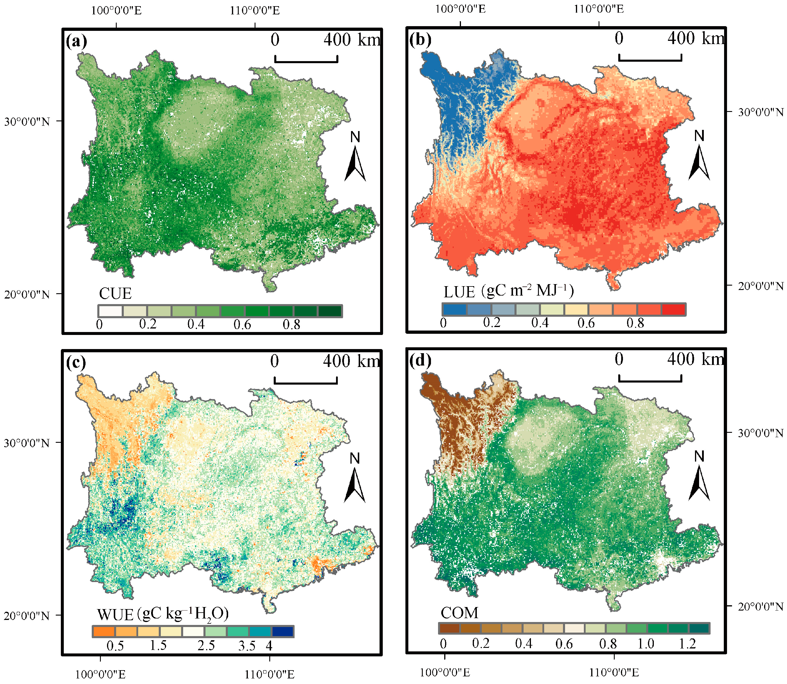
3.1. Spatiotemporal Trends of Ecosystem CUE, LUE, WUE, and COM in Southwest China

From 2000 to 2018, the four types of use efficiencies showed significant spatial heterogeneity in southwest China (Figure 3). Statistically, the average CUE value during the study period was 0.49, with a spatial pattern of high in the southwest and low in the northeast (Figure 3a). For the entire study area, the multi-year average LUE values range from 0 to 1.002 gC m⁻² MJ⁻¹, with a gradual decrease from southeast to northwest (Figure 3b). The pixels with multi-year average values less than 0.5 gC m⁻² MJ⁻¹ were mainly located in western Sichuan. The mean WUE value was 2.31 gC kg⁻¹ H₂O, with high values concentrated in Yunnan and western Guangxi (Figure 3c). For the COM, the multi-year average value was 0.87 and the pixels with average values less than 0.87 accounted for 29.8% of the study area, which were mainly located in the Sichuan Basin, western Sichuan, and eastern Hubei (Figure 3d).

During the study period, the LUE, WUE, and COM showed an increasing trend except for CUE (Figure S3). In southwest China, CUE showed a decreasing trend of 1.3 × 10⁻³ yr⁻¹, with the majority, approximately 61.7%, of the area showing this downward pattern (Figure S4a). Additionally, LUE demonstrated a rise of 1.1 × 10⁻³ gC m⁻² MJ⁻¹ yr⁻¹, predominantly in regions of Guangxi, Guizhou, and northern Guangdong (Figure S4b). For WUE, there was an upward trend of 1.4 × 10⁻² gC kg⁻¹ H₂O yr⁻¹, with 72.03% of the area following this upward trajectory (Figure S4c). For COM, there was a rise of 1.5 × 10⁻³ yr⁻¹, but 29.27% of the region tended to decrease, mainly in western Sichuan and Yunnan (Figure S4d).

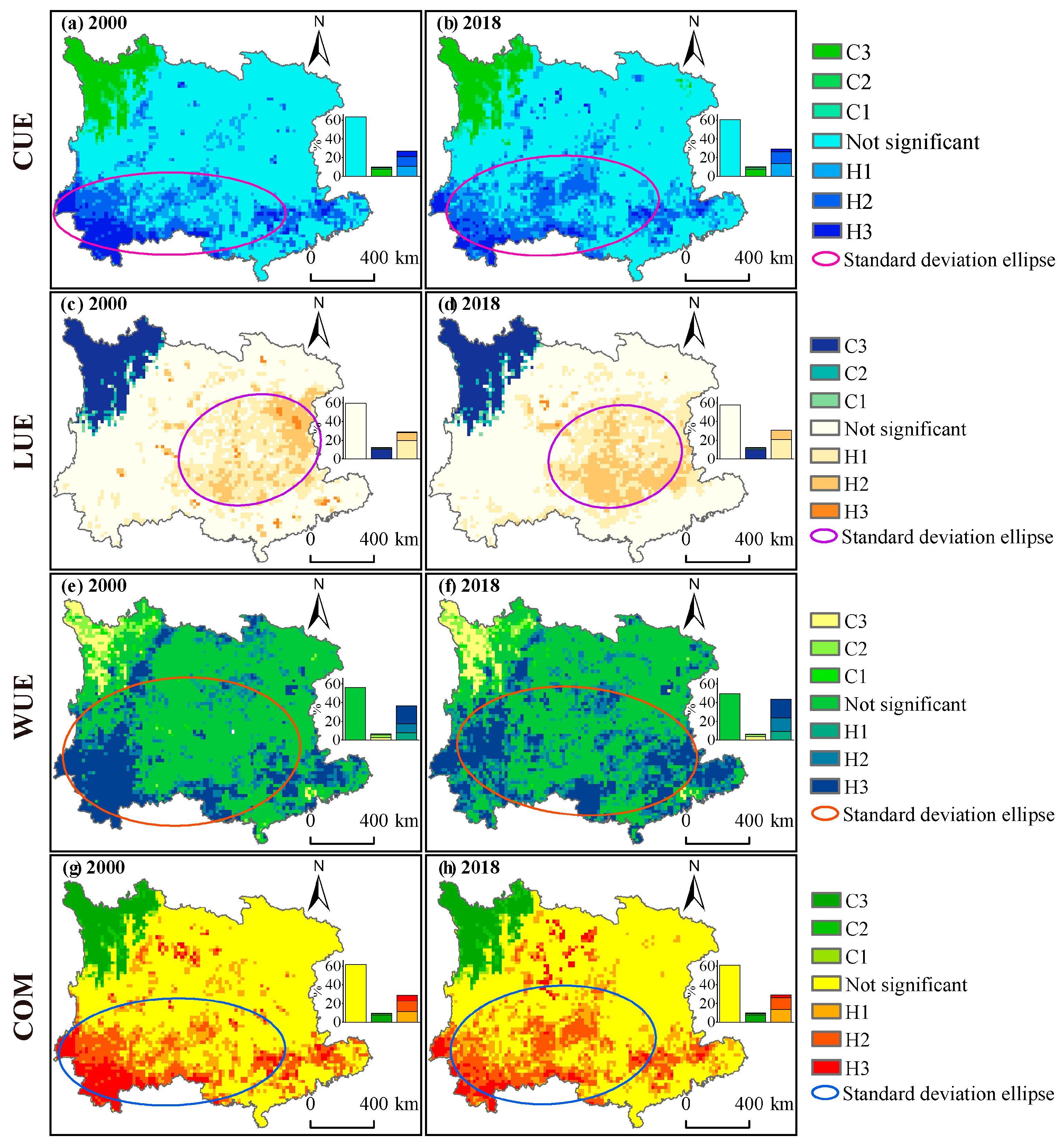
3.2. The Hotspots and Spatial Autocorrelation Characteristics Analysis

From 2000 to 2018, the hotspots of CUE, WUE, and COM were all clustered in the southwest of the study area, such as Yunnan, Guangxi, Guizhou, and northern Guangdong (Figure 4). Hotspots for LUE were primarily found in the eastern region of the study area, such as Guizhou, Hunan, and Guangxi. Compared with 2000, in 2018, the area ratios of hotspot areas for CUE, LUE, WUE, and COM increased from 26.91%, 28.67%, 37.65%, and 28.88% to 29.25%, 30.48%, 44.53%, and 30.73% of the entire area, respectively. The LISA clustering map (Figure S5) accurately represents regions of high and low values for the two-by-two combinations of use efficiency. In 2000 and 2018, for the carbon–light use efficiencies, the high–high value clusters were located mainly in Yunnan and Guizhou, while the low–low value clusters were mainly located in western Sichuan, the Sichuan Basin, and northern Hubei. The spatial divergence of carbon–water has a similarity with carbon–light, the high–high clusters predominated in Yunnan, while western Sichuan, the Sichuan Basin, Hubei, and Hunan were primarily characterized by low–low clusters. The high–high value clusters for light–water were located in southwestern Yunnan, Hunan, Guizhou, and northern Guangxi, and the low–low value areas were identified in western Sichuan.

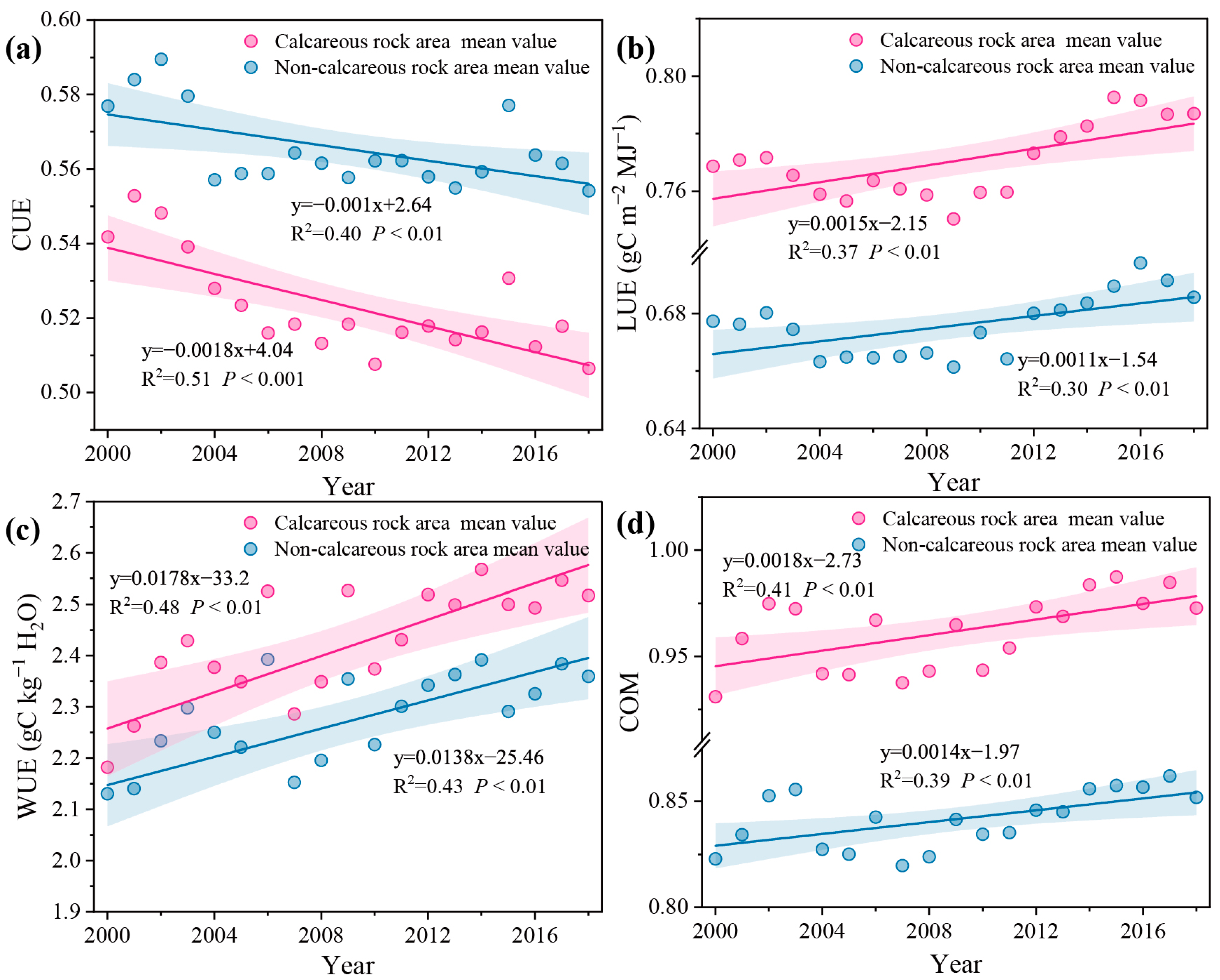
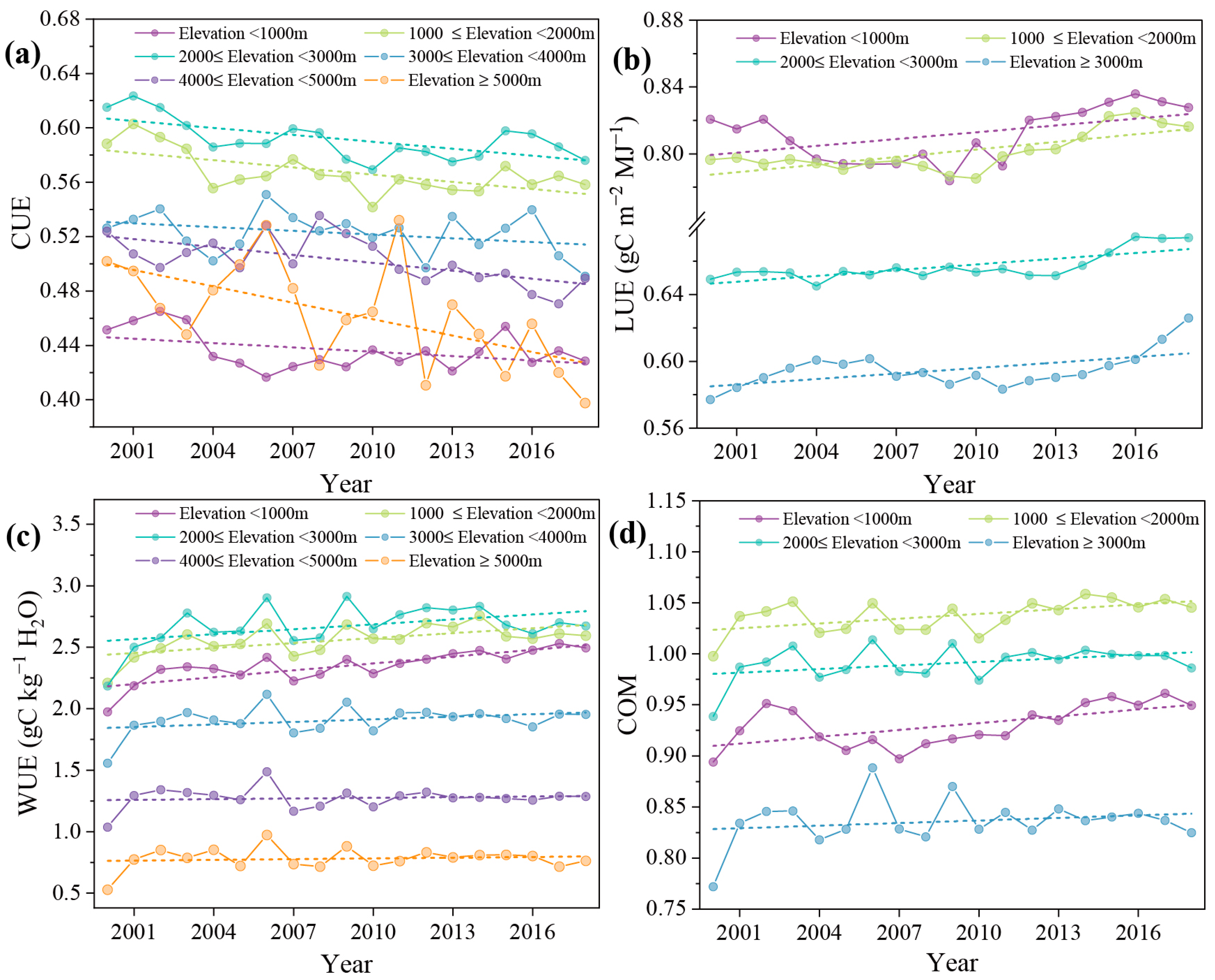
3.3. Divergence Characteristics Analysis under Different Background Conditions

According to the native conditions, each use efficiency in different elevations, rock properties (Figure S6), vegetation cover, and ecological restoration areas exhibited various divergent characteristics. According to statistics, the mean CUE and LUE of the ecological restoration areas were 0.582 and 0.803 gC m⁻² MJ⁻¹, respectively, which were larger than those of the non-ecological restoration areas (0.576 and 0.796 gC m⁻² MJ⁻¹, respectively), but the average WUE and COM were 2.67 gC kg⁻¹ H₂O and 1.058, respectively, both of which were smaller than those of the non-ecological restoration areas (2.79 gC kg⁻¹ H₂O and 1.067, respectively) (Figure S7). From 2000 to 2018, CUE in the non-ecological and ecological restoration areas showed a declining trend, with decreasing trends of −0.0014 yr⁻¹ and −0.0024 yr⁻¹, respectively (Figure 5a). However, LUE, WUE, and COM all trended upwards, with increasing rates of 0.0011 gC m⁻² MJ⁻¹ yr⁻¹ and 0.0016 gC m⁻² MJ⁻¹ yr⁻¹ (Figure 5b), 0.0132 gC kg⁻¹ H₂O yr⁻¹ and 0.0135 gC kg⁻¹ H₂O yr⁻¹ (Figure 5c), and 0.0015 yr⁻¹ and 0.0016 yr⁻¹ (Figure 5d) in the non-ecological and ecological restoration areas, respectively. Generally, the four rates of change in non-ecological restoration areas were consistently lower than those in restored areas.

It was found that the average CUE, WUE, and COM of the calcareous rock areas were 0.54, 2.49 gC kg⁻¹ H₂O, and 1.021, respectively, all of which were lower than those of the non-calcareous rock areas (0.57, 2.74 gC kg⁻¹ H₂O, and 1.054, respectively) (Figure S8). However, the average LUE (0.84 gC m⁻² MJ⁻¹) surpassed that of non-calcareous rock areas (0.82 gC m⁻² MJ⁻¹). Additionally, CUE trended downwards while LUE, WUE, and COM trended upwards in both calcareous and non-calcareous rock areas. For CUE, the decline rates from 2000–2018 were −0.0018 yr⁻¹ and −0.001 yr⁻¹ for calcareous and non-calcareous areas, respectively (Figure 6a). The increase rates of LUE, WUE, and COM were 0.0015 gC m⁻² MJ⁻¹ yr⁻¹ and 0.001 gC m⁻² MJ⁻¹ yr⁻¹ (Figure 6b), 0.0178 gC kg⁻¹ H₂O yr⁻¹ and 0.0138 gC kg⁻¹ H₂O yr⁻¹ (Figure 6c), and 0.0018 yr⁻¹ and 0.0014 yr⁻¹ (Figure 6d) in both calcareous and non-calcareous areas, respectively. The change rates of the four ecosystem use efficiencies were consistently higher in calcareous rock areas than those in non-calcareous rock areas.

Overall, the multi-year average of the four ecosystem use efficiencies initially raised as elevation increased and then declined after a certain elevation threshold (Figure S9). For CUE, WUE, and COM, the multi-year average values reached a peak when the elevation reached approximately 3000 m, and LUE reached its highest value at an elevation of around 1000 m. By comparing the average values of the four use efficiencies of each vegetation type at different elevation gradients, it was found that the CUE, LUE, WUE, and COM of the six vegetation types were varied (Figure S10). Specifically, the average CUE of ENF, DBF, savannas, and crops peaked in the elevation interval of 2000–3000 m, whereas the average CUE of EBF and grasslands showed the peaks of CUE in the region of 1000–2000 m. The average LUE of ENF, DBF, and savannas were highest in the region of below 1000 m, but the highest mean LUE of EBF, grasslands, and crops were observed in the regions of 1000–2000 m. Similarly, grasslands and crops observed the peaks of WUE at elevations of 1000–2000 m, and the highest mean values for the other four vegetation types were all observed at 2000–3000 m. For COM, all of the species of vegetation had the highest mean values in the elevation of 1000–2000 m. This further confirmed that species composition can impact ecosystem use efficiency across elevations.

Moreover, the change rate of each use efficiency exhibited clear differences in various elevation levels for the study area from 2000–2018. For CUE, the elevation gradients above 5000 m and between 3000–4000 m had the largest and smallest change rates, reaching −0.0042 yr⁻¹ and −0.0009 yr⁻¹, respectively (Figure 7a). But LUE had the largest change rate between 1000–2000 m, at 0.0015 gC m⁻² MJ⁻¹ yr⁻¹, and the smallest change rate in the region above 3000 m, at 0.0011 gC m⁻² MJ⁻¹ yr⁻¹ (Figure 7b). For WUE, the most pronounced upward trend was observed below 1000 m, reaching 0.0186 gC kg⁻¹ H₂O yr⁻¹, while the smallest upward trend was noticed at 3000–4000 m, reaching only 0.007 gC kg⁻¹ H₂O yr⁻¹ (Figure 7c). The maximum change rate of COM was observed in the region below 1000 m with 0.0022 yr⁻¹ and the minimum increase rate was found in the region greater than 3000 m with 0.0008 yr⁻¹ (Figure 7d).

The different vegetation types varied considerably in each use efficiency (Figure S11). The vegetation types with the maximum average values for CUE, LUE, and COM were found in EBF, at 0.59, 0.839 gC m⁻² MJ⁻¹, and 1.079, respectively, whereas WUE with the maximum average value was ENF, at 2.88 gC kg⁻¹ H₂O. Meanwhile, the minimum average values for LUE, WUE, and COM were grassland, at 0.217 gC m⁻² MJ⁻¹, 1.322 gC kg⁻¹ H₂O, and 0.425, respectively. The smallest average for CUE was found in crops, at 0.42. In addition, during the study period, various vegetation types demonstrated different change rates in use efficiency (Figure 8). According to the linear regression results, for CUE, there was a decreasing trend for all vegetation types except DBF over the period 2000–2018, with a decline rate ranging from −0.0006 yr⁻¹ to −0.0044 yr⁻¹; the most dramatic change rate was in EBF. For LUE and WUE, all vegetation types trended upwards, and the most significant increase was also observed in EBF with rates of 0.0034 gC m⁻² MJ⁻¹ yr⁻¹ and 0.025 gC kg⁻¹ H₂O yr⁻¹, respectively. For COM, all vegetation types exhibited an increasing trend, with a change rate ranging from 0.001 yr⁻¹ to 0.0037 yr⁻¹; the vegetation type that showed the sharpest change was savannas, with a change trend of 0.0037 yr⁻¹.

3.4. Driving Force Detection of the COM in Southwest China

3.4.1. Selection of the Optimal COM Analysis Scale

To further estimate the influence of scale change on the COM, the descriptive statistical parameters at various scale levels were analyzed by spatial data exploration method (Figure 9). The Z-Score at a 7-level scale was greater than 1.96, indicating a significant spatial clustering of COM (p < 0.05). The spatial autocorrelation Moran’s I values of COM at the sub-basin unit scale were 0.89 and 0.88 in 2000 and 2018, respectively, which were closer to that calculated at the grid unit scale and more pronounced than at the township and county unit scale levels. Meanwhile, the coefficients of variation at the sub-basin unit scale were the highest in the 7-level scale, at 0.39 and 0.4, respectively. Thus, the sub-basin scale was informative in terms of spatial variation in COM, which was a characteristic scale for southwest China.

3.4.2. Independent and Interactive Effects of Driving Forces on the COM

In the study, eight indices were discretized using the equal, natural, quantile, and geometric interval methods (Figures S12 and S13). The OPGD model’s factor detector revealed the significance of explanatory variables relative to each influencer, as detailed in

Table 1. The result of the factor detector for the spatial differentiation from 2000 to 2018.

	Factors	Elevation	Slope	Temperature	Precipitation	Solar Radiation	Vegetation Type	LDCI	Population Density
2000	q-value	0.8055	0.0783	0.8096	0.6036	0.3055	0.2469	0.5329	0.6089
	p-value	0.0000	0.0000	0.0000	0.0000	0.0000	0.0000	0.0000	0.0000
2018	q-value	0.8165	0.0833	0.8233	0.5124	0.2894	0.2773	0.6068	0.5617
	p-value	0.0000	0.0000	0.0000	0.0000	0.0000	0.0000	0.0000	0.0000

. From 2000 to 2018, the explanatory power of LDCI increased from 0.5329 to 0.6068, exceeding population density and precipitation. Furthermore, the q-values of precipitation, solar radiation, and population density decreased. Comparing q-values between 2000 and 2018 revealed distinct changes in separate factors across different years. Temperature consistently emerged as a dominant factor for COM, displaying a significant impact. The influencing power of topographic factors (elevation and slope), vegetation types, and LDCI continued to increase, pointing to an increasing effect of natural factors on COM.

The analysis of factor interactions affecting COM spatial variability in southwest China, depicted in Figure 10, indicates significance through p-values. Notably, q-values from factor pairs generally exceed those of standalone factors, underscoring the amplified influence of combined factors. In both 2000 and 2018, it was found that elevation and temperature demonstrated the most pronounced effect, with q-values of 0.8713 and 0.8779, respectively; interactions involving elevation or temperature with other factors consistently yielded q-values above 0.8. It illustrated that temperature and elevation interacted with other factors and markedly enhanced the explanatory power of spatial variation in COM for the study area. Over the two periods, the explanatory power of population density interacted with other factors above 0.6, which was obviously stronger than its single-factor explanatory power.

3.4.3. Interaction of Driving Factors for COM Divergence

The single-factor analysis revealed that several factors possess explanatory capacities for COM exceeding 50%. These included elevation, temperature, precipitation, LDCI, and population density. These factors were standardized and then coupled in pairs to understand their combined spatial influences on COM. Spatially, the coupling of temperature–precipitation, temperature–elevation, and temperature–LDCI on COM was generally stronger in the northwest and showed a gradational decline toward the southeast. Notably, the beneficial impacts were primarily observed in the western Sichuan Plateau and its periphery. The coupling of elevation–precipitation, and elevation–LDCI on COM showed a trend of negative correlation from northwest to positive correlation from southeast, and the strongest negative effect was also concentrated in the western Sichuan Plateau (Figure 11). The coupling of elevation–temperature had lower spatial explanatory power, and precipitation–population density had higher driving power. Overall, about 39.7% of the region was dominated by the coupling of precipitation–population density, predominantly in the western region, and approximately 44.4% of the area was mainly influenced by the coupling of elevation–population density, mainly in the eastern region.

4. Discussion

4.1. Trade-Offs/Synergies among Water–Carbon–Light Use Efficiencies

The anti-disturbance ability and resource use efficiency of plant communities are critical elements in their adaptation to environmental changes and resistance to external stresses, and they jointly determine the stability and survivability of plant communities. COM, as a comprehensive index of independent efficiencies (CUE, WUE, and LUE), can comprehensively evaluate the vegetation’s ability to coordinate multiple efficiencies, and its value is directly associated with ecosystem functionality and stability [61]. It was found that despite the CUE showing a decreasing trend from 2000 to 2018, the WUE and LUE of vegetation increased, which contributed to the overall positive trend of COM. These indicated that although plants face challenges in maintaining efficient carbon fixation during photosynthesis, by adapting physiological and morphological characteristics, plants are able to accommodate environmental changes and maintain or even enhance overall ecosystem functioning. Previous research has indicated that over the past two decades, the southwestern region has undergone significant climatic warming, with a temperature increase rate of 0.1–0.3 °C yr⁻¹, marking the warmest period since the 1960s [14]. This has led to environmental stresses such as drought and high temperatures, which have intensified plant respiration and may lead to a decrease in CUE [62,63]. However, plants have adapted to these stresses by adjusting stomatal conductance, optimizing water use strategies, and altering leaf structure and chlorophyll content, thereby enhancing WUE and LUE [64,65]. Furthermore, a series of ecological restoration projects have been implemented in southwestern China over the past 20 years, such as Grain for Green and Natural Forests Protection [33]. These projects have increased vegetation cover and biodiversity, turning the region into a global hotspot for the “greening” of vegetation, contributing 5% of the global above-ground biomass with only 0.36% of the global lands [66]. Therefore, vegetation restoration and reconstruction have positively impacted the integrated vegetation water–carbon–light use efficiency.

The multi-year mean value of vegetation COM was 0.87, but there was significant heterogeneity in the spatial distribution. Using the Getis-Ord Gi* statistic and the spatial overlay of the two efficiencies, the Yunnan–Guizhou Plateau was found to be a hotspot area for COM. This is primarily ascribed to the synergistic effect of CUE and WUE, and CUE and LUE in this region. Owing to the abundant precipitation in the region, where water availability is not a limiting factor for vegetation growth, the complex plateau landscape provides a microenvironment for various plants, which enhances carbon fixation [66]. Meanwhile, the high elevation exposes the plants to more solar radiation, which facilitates enhanced photosynthetic activity and light energy capture [67]. Conversely, the Western Sichuan Plateau was a coldspot region for COM, and also had a slower growth rate over the study period than the rest of the region, indicating low-level coordination of these three use efficiencies. This phenomenon may be attributed to the lack of water availability caused by the uneven distribution of precipitation and groundwater resources, restricting plant growth and photosynthesis [68]. Moreover, the soil in the western Sichuan Plateau is generally poor, lacking nutrients and organic matter, and large areas of bare ground and sparse vegetation further limit vegetation, thus impairing carbon sequestration and hindering productivity [39,69]. Although the southeastern part was the hotspot region for LUE and WUE in the study area, the trade-off of CUE with CUE and WUE made it the coldspot region for COM. Overall, these spatial characteristics of COM highlight the intricate interactions between environmental conditions, resource use efficiency, and vegetation’s adaptive strategies across different regions. In the future, the physiological and ecological processes behind vegetation’s integrated water, carbon, and light capacities can be analyzed in detail to understand more clearly the response mechanisms of vegetation to multiple environmental factors.

4.2. Ecological Restoration Enlightenment Based on Divergent Characteristics

Although vegetation restoration is beneficial in halting the stone desertification process in karst ecosystems, the surface of the area consists mainly of exposed rock and limestone, and soils are usually shallow and vegetation is stressed by soil nutrients and has a weaker capacity to sequester carbon. For karst areas as a whole, the CUE was still lower compared to non-karst areas [70,71]. It has been recommended that grassland instead of forest should be preferred as the dominant vegetation type for ecological restoration of karst landscapes [66,72,73]. However, further analysis in this study revealed that grassland had a lower COM value compared to other vegetation types. Therefore, from the perspective of enhancing the overall COM of the region, grasslands are not suitable as a vegetation type for ecological restoration. On the contrary, broadleaved evergreen forests have higher COM and should be prioritized with drought-tolerant tree species, such as Acacia and Toona sinensis, which can withstand cold, drought, and infertile soils, and can be better adapted to high calcium environments [74].

In the past, substantial investment has been made from the perspective of soil and water conservation and improvement in vegetation coverage, which has enhanced the COM of ecological restoration areas. However, during the ecological recovery process in artificial forests, the cultivation of a single dominant plant species has led to reduced vegetation coverage and a significant decline in biodiversity [75]. Moreover, a lack of recognition of the value of ecological products, problems such as the imbalance between supply and demand, and the disconnection between ecological and economic benefits have also hindered the development of karst areas [76]. Therefore, future development strategies should aim to reduce indiscriminate large-scale afforestation and prioritize the protection of existing natural forestlands and arable resources, rather than short-term green expansion. By employing principles of natural resource management and landscape ecology, efforts should be directed toward the development and cultivation of high-quality local tree species, increasing the species diversity in artificial forests, and gradually establishing a stable supply system for ecological products.

Considering the internal variability of the topography in karst regions, a zoning strategy is crucial for guiding the spatial layout and methods of vegetation restoration. It is recommended to develop specific ecological plans based on different landforms, such as peak cluster depressions, valley types, plateaus, and gorges, in conjunction with the environmental characteristics. Meanwhile, there is a threshold effect between COM of different vegetation types and elevation, which necessitates the adoption of a three-dimensional planting model. For instance, at the bottom of depressions with frequent human activities, dryland farming should be dominated. In the economically underdeveloped foothills and gentle slopes, there should be a focus on developing high-quality fruit trees, economic forests, and timber forests, interspersed with medicinal plants [74]. On ridge tops and steep slopes, emphasis should be placed on developing vine plants such as Honeysuckle, with appropriate cultivation of bamboo [77,78]. Through these measures, a multidimensional agroforestry system can be established, ranging from depressions to mountain tops, encompassing “fruits–economy–forestry”, to achieve both ecological and economic benefits.

4.3. Impact of Temperature, Elevation, and Coupling Factor on COM

The COM’s reaction to a range of influences such as climate conditions, geographical features, and human actions hinges on the primary factors that govern plant photosynthesis, ecosystem water evaporation, and shifts in the carbon cycle dynamics [3] (Xiao et al., 2023). The results of the OPGD model assessment revealed that temperature and elevation had a greater influence on the COM variability [79], which is in accordance with other studies [80,81]. With global warming, respiration may exceed the photosynthetic rate, disrupting the carbon balance [82,83]. Therefore, more effective measures should be taken in the future to keep the global temperature within a certain range, which can increase the vegetation COM. In our study, the COM in southwest China exhibited significant vertical variations; they rose to a peak and subsequently diminished as elevation gained, registering maximum values around 3000 m. This confirmed the results of the spatial analysis that higher elevation in western Sichuan showed a significantly weak negative correlation to COM. When elevation exceeds a certain threshold, CO₂ concentration decreases, and the fractionation of 13C by leaves during photosynthesis reduces, resulting in an enriched stable carbon isotope composition of photosynthesis products, which leads to a lower WUE [84,85].

The interactive effect of any two factors on COM was found to be greater than that of one individual factor, which was also confirmed spatially. Previous studies have emphasized that the synergy of anthropogenic practices and environmental elements significantly influences vegetation development. For example, Zhu et al. (2023) [86] discovered that climate variation and human interventions accounted for 59.68% and 40.32% of the increase in vegetation lushness within the Liaohe River Basin, with changes in precipitation being the main factor influencing vegetation cover change; Li et al. (2021) [87] concluded that natural and anthropogenic drivers have a strong dynamic coupling relationship with vegetation ecosystem services. Our study in southwest China showed that 39.7% and 44.4% of the region’s COM were dominated by the interaction of precipitation–population density and elevation–population density, respectively. This further illustrates that the coupling of regional natural conditions and human activity is decisive for the divergent characteristics of vegetation use efficiency.

4.4. Limitations and Perspectives of This Study

For karst regions, the carbon sink is not limited to soil and vegetation; the process of rock weathering also contributes significantly to the formation of carbon sinks [88,89]. In the future, carbon sinks generated by rock weathering processes should be taken into account when calculating CUE. The OPGD model can reveal the interactions between different environmental factors on vegetation. However, limited by the available data, only eight indicators including natural and anthropogenic factors were considered in this study, which failed to adequately consider other factors such as nutrient use efficiency that have an impact on vegetation COM. In the future, the indicator selection should be improved and multiple methods, such as principal component analysis (PCA), should be used to generalize multiple factors into a composite factor in order to improve the accuracy of exploring the driving mechanism of vegetation COM. Moreover, in the future, the OPGD model can be combined with other statistical models and machine learning algorithms to predict the adaptive capacity and resilience of vegetation under environmental changes by using long-term ecological monitoring data, so as to provide a scientific basis for ecosystem management and protection.

5. Conclusions

This study revealed the spatial heterogeneity of the CUE, LUE, WUE, and COM in southwest China from 2000 to 2018. Then, the spatial driving mechanism of COM was investigated based on the optimal scale. The results demonstrated significant spatial variability among the four use efficiencies. Notably, hotspots of LUE were primarily concentrated in Hubei and Guizhou provinces in the eastern part of the study area, while the vegetation in the Yunnan–Guizhou Plateau generally exhibited higher CUE, WUE, and COM, compared to the western Sichuan Plateau, which showed a coldspot region for all four use efficiencies. During 2000–2018, the vegetation’s CUE showed a decrease at a rate of 1.3 × 10⁻³ yr⁻¹, while the enhanced trends of LUE and WUE collectively contributed to a positive change in COM. Additionally, exploratory spatial analysis results indicated that the spatial aggregation of vegetation use efficiency was most pronounced at the sub-basin scale. At this scale, it revealed that temperature consistently emerged as the primary factor influencing the variation in vegetation COM. Compared with 2000, the impact of topographical factors, vegetation types, and human activities on COM has been continuously strengthening. Moreover, the interaction of multiple factors, particularly the coupling of elevation/precipitation with population density, significantly enhanced the explanatory power for the spatial differentiation of COM. Future regional ecological management policies should fully consider the variability in efficiency within the region and delve into the underlying mechanisms. This will aid in providing a scientific basis and strategic support for ecological conservation and green development in the southwestern region and beyond.

References

1. Huang, M.T.; Piao, S.L.; Sun, Y.; Ciais, P.; Cheng, L.; Mao, J.F.; Wang, Y.P. Change in terrestrial ecosystem water-use efficiency over the last three decades. Glob. Chang. Biol. 2015, 21, 2366–2378. [Google Scholar] [CrossRef] [PubMed]
2. Keenan, T.F.; Hollinger, D.Y.; Bohrer, G.; Dragoni, D.; Munger, J.W.; Schmid, H.P.; Richardson, A.D. Increase in forest water-use efficiency as atmospheric carbon dioxide concentrations rise. Nature 2013, 499, 324–327. [Google Scholar] [CrossRef]
3. Xiao, B.Q.; Bai, X.Y.; Zhao, C.W.; Tan, Q.; Li, Y.B.; Luo, G.J.; Du, C.C. Responses of carbon and water use efficiencies to climate and land use changes in China’s karst areas. J. Hydrol. 2023, 617, 13. [Google Scholar] [CrossRef]
4. Bradford, M.A.; Crowther, T.W. Carbon use efficiency and storage in terrestrial ecosystems. New Phytol. 2013, 199, 7–9. [Google Scholar] [CrossRef] [PubMed]
5. Hou, G.; Sun, J.; Wang, J.N. Dynamics and Controls of Carbon Use Efficiency across China’s Grasslands. Pol. J. Environ. Stud. 2018, 27, 1541–1550. [Google Scholar] [CrossRef] [PubMed]
6. Wang, L.M.; Li, M.Y.; Wang, J.X.; Li, X.G.; Wang, L.C. An analytical reductionist framework to separate the effects of climate change and human activities on variation in water use efficiency. Sci. Total Environ. 2020, 727, 15. [Google Scholar] [CrossRef] [PubMed]
7. Xue, Y.Y.; Liang, H.B.; Zhang, B.Q.; He, C.S. Vegetation restoration dominated the variation of water use efficiency in China. J. Hydrol. 2022, 612, 14. [Google Scholar] [CrossRef]
8. Gitelson, A.A.; Gamon, J.A. The need for a common basis for defining light-use efficiency: Implications for productivity estimation. Remote Sens. Environ. 2015, 156, 196–201. [Google Scholar] [CrossRef]
9. Pangle, L.; Vose, J.M.; Teskey, R.O. Radiation use efficiency in adjacent hardwood and pine forests in the southern Appalachians. For. Ecol. Manag. 2009, 257, 1034–1042. [Google Scholar] [CrossRef]
10. Fei, X.H.; Song, Q.H.; Zhang, Y.P.; Yu, G.R.; Zhang, L.M.; Sha, L.Q.; Grace, J. Patterns and Controls of Light Use Efficiency in Four Contrasting Forest Ecosystems in Yunnan, Southwest China. J. Geophys. Res. Biogeosciences 2019, 124, 293–311. [Google Scholar] [CrossRef]
11. Flexas, J.; Barbour, M.M.; Brendel, O.; Cabrera, H.M.; Carriquí, M.; Díaz-Espejo, A.; Warren, C.R. Mesophyll diffusion conductance to CO2: An unappreciated central player in photosynthesis. Plant Sci. 2012, 193, 70–84. [Google Scholar] [CrossRef] [PubMed]
12. Piao, S.; Friedlingstein, P.; Ciais, P.; de Noblet-Ducoudré, N.; Labat, D.; Zaehle, S. Changes in climate and land use have a larger direct impact than rising CO2 on global river runoff trends. Proc. Natl. Acad. Sci. USA 2007, 104, 15242–15247. [Google Scholar] [CrossRef] [PubMed]
13. Wang, J.; Wen, X.F.; Zhang, X.Y.; Li, S.G. The strategies of water-carbon regulation of plants in a subtropical primary forest on karst soils in China. Biogeosciences 2018, 15, 4193–4203. [Google Scholar] [CrossRef]
14. Zhang, J.; Yang, S.Q.; Yang, S.T.; Fan, L.; Zhou, X. Spatio-Temporal Variations of Ecosystem Water Use Efficiency and Its Drivers in Southwest China. Land 2023, 12, 397. [Google Scholar] [CrossRef]
15. Geekiyanage, N.; Goodale, U.M.; Cao, K.F.; Kitajima, K. Plant ecology of tropical and subtropical karst ecosystems. Biotropica 2019, 51, 626–640. [Google Scholar] [CrossRef]
16. Zhang, Y.J.; Yu, G.R.; Yang, J.; Wimberly, M.C.; Zhang, X.Z.; Tao, J.; Zhu, J.T. Climate-driven global changes in carbon use efficiency. Glob. Ecol. Biogeogr. 2014, 23, 144–155. [Google Scholar] [CrossRef]
17. Piao, S.; Luyssaert, S.; Ciais, P.; Janssens, I.A.; Chen, A.; Cao, C.; Wang, S. Forest annual carbon cost: A global-scale analysis of autotrophic respiration. Ecology 2010, 91, 652–661. [Google Scholar] [CrossRef] [PubMed]
18. Qu, R.; Han, G.L. Effects of high Ca and Mg stress on plants water use efficiency in a Karst ecosystem. PeerJ 2022, 10, 14. [Google Scholar] [CrossRef] [PubMed]
19. Si, J.H.; Feng, Q.; Yu, T.F.; Zhao, C.Y.; Li, W. Variation in populus euphratica foliar carbon isotope composition and osmotic solute for different groundwater depths in an arid region of China. Environ. Monit. Assess. 2015, 187, 15. [Google Scholar] [CrossRef]
20. Zhang, S.B.; Zhang, J.L.; Slik, J.W.F.; Cao, K.F. Leaf element concentrations of terrestrial plants across China are influenced by taxonomy and the environment. Glob. Ecol. Biogeogr. 2012, 21, 809–818. [Google Scholar] [CrossRef]
21. Ding, Z.; Liu, Y.; Wang, L.C.; Chen, Y.A.; Yu, P.J.; Ma, M.G.; Tang, X.G. Effects and implications of ecological restoration projects on ecosystem water use efficiency in the karst region of Southwest China. Ecol. Eng. 2021, 170, 9. [Google Scholar] [CrossRef]
22. Gao, Y.; Zhu, X.J.; Yu, G.R.; He, N.P.; Wang, Q.F.; Tian, J. Water use efficiency threshold for terrestrial ecosystem carbon sequestration in China under afforestation. Agric. For. Meteorol. 2014, 195, 32–37. [Google Scholar] [CrossRef]
23. Zhang, M.Y.; Wang, K.L.; Liu, H.Y.; Wang, J.; Zhang, C.H.; Yue, Y.M.; Qi, X.K. Spatio-Temporal Variation and Impact Factors for Vegetation Carbon Sequestration and Oxygen Production Based on Rocky Desertification Control in the Karst Region of Southwest China. Remote Sens. 2016, 8, 102. [Google Scholar] [CrossRef]
24. Hou, Y.; Li, B.; Müller, F.; Fu, Q.; Chen, W.P. A conservation decision-making framework based on ecosystem service hotspot and interaction analyses on multiple scales. Sci. Total Environ. 2018, 643, 277–291. [Google Scholar] [CrossRef]
25. Rabe, S.E.; Koellner, T.; Marzelli, S.; Schumacher, P.; Grêt-Regamey, A. National ecosystem services mapping at multiple scales—The German exemplar. Ecol. Indic. 2016, 70, 357–372. [Google Scholar] [CrossRef]
26. Han, R.Y.; Wang, Z.H.; Shen, Y.Y.; Wu, Q.X.; Liu, X.M.; Cao, C.; Zhang, J. Anthropogenic Gd in urban river water: A case study in Guiyang, SW China. Elementa Sci. Anthrop. 2021, 9, 13. [Google Scholar] [CrossRef]
27. Yue, Y.; Wang, K.; Zhang, B.; Jiao, Q.; Liu, B.; Zhang, M. Remote sensing of fractional cover of vegetation and exposed bedrock for karst rocky desertification assessment. Procedia Environ. Sci. 2012, 13, 847–853. [Google Scholar] [CrossRef]
28. Chen, Y.J.; Cao, K.F.; Schnitzer, S.A.; Fan, Z.X.; Zhang, J.L.; Bongers, F. Water-use advantage for lianas over trees in tropical seasonal forests. New Phytol. 2015, 205, 128–136. [Google Scholar] [CrossRef] [PubMed]
29. Nie, Y.P.; Chen, H.S.; Wang, K.L.; Ding, Y.L. Seasonal variations in leaf δ 13 C values: Implications for different water-use strategies among species growing on continuous dolomite outcrops in subtropical China. Acta Physiol. Plant 2014, 36, 2571–2579. [Google Scholar] [CrossRef]
30. Wang, S.J.; Liu, Q.M.; Zhang, D.F. Karst rocky desertification in southwestern China: Geomorphology, landuse, impact and rehabilitation. Land Degrad. Dev. 2004, 15, 115–121. [Google Scholar] [CrossRef]
31. Chen, T.T.; Wang, Q.; Wang, Y.X.; Peng, L. Processes and mechanisms of vegetation ecosystem responding to climate and ecological restoration in China. Front. Plant Sci. 2022, 13, 14. [Google Scholar] [CrossRef] [PubMed]
32. Peng, L.; Chen, T.T.; Deng, W.; Liu, Y. Exploring ecosystem services trade-offs using the Bayesian belief network model for ecological restoration decision-making: A case study in Guizhou Province, China. Ecol. Indic. 2022, 135, 11. [Google Scholar] [CrossRef]
33. Yue, Y.M.; Qi, X.K.; Wang, K.L.; Liao, C.J.; Tong, X.W.; Brandt, M.; Liu, B. Large scale rocky desertification reversal in South China karst. Prog. Phys. Geogr. 2022, 46, 661–675. [Google Scholar] [CrossRef]
34. Huang, L.; He, B.; Han, L.; Liu, J.J.; Wang, H.Y.; Chen, Z.Y. A global examination of the response of ecosystem water-use efficiency to drought based on MODIS data. Sci. Total Environ. 2017, 601, 1097–1107. [Google Scholar] [CrossRef] [PubMed]
35. Yin, J.B.; Gentine, P.; Slater, L.; Gu, L.; Pokhrel, Y.; Hanasaki, N.; Schlenker, W. Future socio-ecosystem productivity threatened by compound drought-heatwave events. Nat. Sustain. 2023, 6, 259–272. [Google Scholar] [CrossRef]
36. Zhang, C.H.; Qi, X.K.; Wang, K.L.; Zhang, M.Y.; Yue, Y.M. The application of geospatial techniques in monitoring karst vegetation recovery in southwest China: A review. Prog. Phys. Geogr. 2017, 41, 450–477. [Google Scholar] [CrossRef]
37. Li, P.L.; Zhu, D.; Wang, Y.L.; Liu, D. Elevation dependence of drought legacy effects on vegetation greenness over the Tibetan Plateau. Agric. For. Meteorol. 2020, 295, 12. [Google Scholar] [CrossRef]
38. Pan, N.Q.; Feng, X.M.; Fu, B.J.; Wang, S.; Ji, F.; Pan, S.F. Increasing global vegetation browning hidden in overall vegetation greening: Insights from time-varying trends. Remote Sens. Environ. 2018, 214, 59–72. [Google Scholar] [CrossRef]
39. Peng, W.F.; Kuang, T.T.; Tao, S. Quantifying influences of natural factors on vegetation NDVI changes based on geographical detector in Sichuan, western China. J. Clean. Prod. 2019, 233, 353–367. [Google Scholar] [CrossRef]
40. Chen, J.; Brissette, F.P.; Leconte, R. Uncertainty of downscaling method in quantifying the impact of climate change on hydrology. J. Hydrol. 2011, 401, 190–202. [Google Scholar] [CrossRef]
41. Cogswell, A.; Greenan, B.J.W.; Greyson, P. Evaluation of two common vulnerability index calculation methods. Ocean Coast. Manag. 2018, 160, 46–51. [Google Scholar] [CrossRef]
42. Liu, Y.; Li, P.; Wang, Y.X.; Xu, X.Y. Quantification of carbon-water dynamics in soil-perennial grass (Bothriochloa ischaemum) feedbacks under drought stress following a double isotope-labelled pulse experiment. Agric. For. Meteorol. 2023, 329, 13. [Google Scholar] [CrossRef]
43. Yuan, W.; Liu, S.; Zhou, G.; Zhou, G.; Tieszen, L.L.; Baldocchi, D.; Goulden, M.L. Deriving a light use efficiency model from eddy covariance flux data for predicting daily gross primary production across biomes. Agric. For. Meteorol. 2007, 143, 189–207. [Google Scholar] [CrossRef]
44. Xiao, X.M.; Zhang, Q.Y.; Braswell, B.; Urbanski, S.; Boles, S.; Wofsy, S.; Berrien, M.; Ojima, D. Modeling gross primary production of temperate deciduous broadleaf forest using satellite images and climate data. Remote Sens. Environ. 2004, 91, 256–270. [Google Scholar] [CrossRef]
45. Yuan, W.P.; Zheng, Y.; Piao, S.L.; Ciais, P.; Lombardozzi, D.; Wang, Y.P.; Yang, S. Increased atmospheric vapor pressure deficit reduces global vegetation growth. Sci. Adv. 2019, 5, 12. [Google Scholar] [CrossRef] [PubMed]
46. Dong, J.; Lu, H.B.; Wang, Y.W.; Ye, T.; Yuan, W.P. Estimating winter wheat yield based on a light use efficiency model and wheat variety data. ISPRS J. Photogramm. Remote Sens. 2020, 160, 18–32. [Google Scholar] [CrossRef]
47. Getis, A.; Ord, J.K. The analysis of spatial association by use of distance statistics. Geogr. Anal. 1992, 24, 189–206. [Google Scholar] [CrossRef]
48. Wan, J.J.; Wang, Z.M.; Ma, C.C.; Su, Y.; Zhou, T.; Wang, T.T.; Tang, X.H. Spatial-temporal differentiation pattern and influencing factors of high-quality development in counties: A case of Sichuan, China. Ecol. Indic. 2023, 148, 17. [Google Scholar] [CrossRef]
49. Anselin, L. Local indicators of spatial association-LISA. Geogr. Anal. 1995, 27, 93–115. [Google Scholar] [CrossRef]
50. Sun, J.H.; Guo, E.R.; Yang, X.T.; Kong, Y.H.; Yang, L.; Liu, H.; Lin, X.B. Seasonal and spatial variations in soil biochemical properties in areas with different degrees of mining subsidence in Central China. Catena 2023, 224, 15. [Google Scholar] [CrossRef]
51. Xiao, R.; Cao, W.; Liu, Y.; Lu, B.B. The impacts of landscape patterns spatio-temporal changes on land surface temperature from a multi-scale perspective: A case study of the Yangtze River Delta. Sci. Total Environ. 2022, 821, 11. [Google Scholar] [CrossRef] [PubMed]
52. Zhou, W.; Yang, K.; Bai, Z.K.; Cheng, H.X.; Liu, F. The development of topsoil properties under different reclaimed land uses in the Pingshuo opencast coalmine of Loess Plateau of China. Ecol. Eng. 2017, 100, 237–245. [Google Scholar] [CrossRef]
53. Wang, J.F.; Zhang, T.L.; Fu, B.J. A measure of spatial stratified heterogeneity. Ecol. Indic. 2016, 67, 250–256. [Google Scholar] [CrossRef]
54. Zhang, K.; Lü, Y.H.; Fu, B.J.; Li, T. The effects of restoration on vegetation trends: Spatiotemporal variability and influencing factors. Earth Environ. Sci. Trans. R. Soc. Edinb. 2019, 109, 473–481. [Google Scholar] [CrossRef]
55. He, L.; Guo, J.; Jiang, Q.; Zhang, Z.; Yu, S. How did the Chinese Loess Plateau turn green from 2001 to 2020? An explanation using satellite data. Catena 2022, 214, 106246. [Google Scholar] [CrossRef]
56. Yang, L.S.; Feng, Q.; Wen, X.H.; Barzegar, R.; Adamowski, J.F.; Zhu, M.; Yin, Z.L. Contributions of climate, elevated atmospheric CO2 concentration and land surface changes to variation in water use efficiency in Northwest China. Catena 2022, 213, 15. [Google Scholar] [CrossRef]
57. Wang, M.; Wang, Y.; Wu, Y.M.; Yue, X.L.; Wang, M.J.; Hu, P.P. Identifying the spatial heterogeneity in the effects of the construction land scale on carbon emissions: Case study of the Yangtze River Economic Belt, China. Environ. Res. 2020, 212, 12. [Google Scholar] [CrossRef] [PubMed]
58. Tian, H.J.; Cao, C.X.; Chen, W.; Bao, S.N.; Yang, B.; Myneni, R.B. Response of vegetation activity dynamic to climatic change and ecological restoration programs in Inner Mongolia from 2000 to 2012. Ecol. Eng. 2015, 82, 276–289. [Google Scholar] [CrossRef]
59. Guo, L.; Luo, M.; Zhangyang, C.S.; Zeng, C.; Wang, S.Q.; Zhang, H.T. Spatial modelling of soil organic carbon stocks with combined principal component analysis and geographically weighted regression. J. Agric. Sci. 2018, 156, 774–784. [Google Scholar] [CrossRef]
60. Zhang, X.M.; Yue, Y.M.; Tong, X.W.; Wang, K.L.; Qi, X.K.; Deng, C.X.; Brandt, M. Eco-engineering controls vegetation trends in southwest China karst. Sci. Total Environ. 2021, 770, 12. [Google Scholar] [CrossRef]
61. Zhang, L.X.; Zhou, D.C.; Fan, J.W.; Hu, Z.M. Comparison of four light use efficiency models for estimating terrestrial gross primary production. Ecol. Model. 2015, 300, 30–39. [Google Scholar] [CrossRef]
62. Norby, R.J.; Zak, D.R. Ecological Lessons from Free-Air CO2 Enrichment (FACE) Experiments. Annu. Rev. Ecol. Evol. Syst. 2011, 44, 181–203. [Google Scholar] [CrossRef]
63. Thomas, R.T.; Prentice, L.C.; Graven, H.; Ciais, P.; Fisher, J.B.; Hayes, D.J.; Zeng, N. Increased light-use efficiency in northern terrestrial ecosystems indicated by CO2 and greening observations. Geophys. Res. Lett. 2016, 43, 11339–11349. [Google Scholar] [CrossRef]
64. Wang, M.; Ding, Z.; Wu, C.Y.; Song, L.S.; Ma, M.G.; Yu, P.J.; Tang, X.G. Divergent responses of ecosystem water-use efficiency to extreme seasonal droughts in Southwest China. Sci. Total Environ. 2020, 760, 14. [Google Scholar] [CrossRef]
65. Zhang, Q.; Lu, J.X.; Xu, X.X.; Ren, X.Z.; Wang, J.F.; Chai, X.H.; Wang, W.W. Spatial and Temporal Patterns of Carbon and Water Use Efficiency on the Loess Plateau and Their Influencing Factors. Land 2023, 12, 77. [Google Scholar] [CrossRef]
66. Tong, X.W.; Wang, K.L.; Brandt, M.; Yue, Y.M.; Liao, C.J.; Fensholt, R. Assessing Future Vegetation Trends and Restoration Prospects in the Karst Regions of Southwest China. Remote Sens. 2016, 8, 357. [Google Scholar] [CrossRef]
67. Wang, J.; Wang, K.L.; Zhang, M.Y.; Zhang, C.H. Impacts of climate change and human activities on vegetation cover in hilly southern China. Ecol. Eng. 2015, 81, 451–461. [Google Scholar] [CrossRef]
68. Keyimu, M.; Li, Z.S.; Wu, X.C.; Fu, B.J.; Liu, G.H.; Shi, S.L.; Wang, X.C. Recent decline of high altitude coniferous growth due to thermo-hydraulic constrains: Evidence from the Miyaluo Forest Reserve, Western Sichuan Plateau of China. Dendrochronologia 2020, 63, 8. [Google Scholar] [CrossRef]
69. Xie, D.; Liu, X.Q.; Chen, Y.X.; Jiao, D.; Lou, J.X.; Qiu, X.F.; Wang, X.Q. Distribution and conservation of threatened gymnosperms in China. Glob. Ecol. Conserv. 2021, 32, 11. [Google Scholar] [CrossRef]
70. Bai, X.Y.; Zhang, S.R.; Li, C.J.; Xiong, L.; Song, F.J.; Du, C.C.; Wang, S.J. A carbon-neutrality-capactiy index for evaluating carbon sink contributions. Environ. Sci. Ecol. 2023, 15, 12. [Google Scholar] [CrossRef]
71. Niu, Q.F.; Xiao, X.M.; Zhang, Y.; Qin, Y.W.; Dang, X.H.; Wang, J.; Zhou, X.M. Ecological engineering projects increased vegetation cover, production, and biomass in semiarid and subhumid Northern China. Land Degrad. Dev. 2019, 30, 1620–1631. [Google Scholar] [CrossRef]
72. Yu, G.R.; Wang, Q.F.; Zhuang, J. Modeling the water use efficiency of soybean and maize plants under environmental stresses: Application of a synthetic model of photosynthesis-transpiration based on stomatal behavior. J. Plant Physiol. 2004, 161, 303–318. [Google Scholar] [CrossRef]
73. Zuo, L.Y.; Gao, J.B. Dynamic analysis of the determinants of trade-off and synergy between karst soil loss and water yield with integration of geomorphological differentiation. Ecol. Indic. 2022, 137, 13. [Google Scholar] [CrossRef]
74. Yang, J.; Xu, X.L.; Liu, M.X.; Xu, C.H.; Zhang, Y.H.; Luo, W.; Wang, K.L. Effects of “Grain for Green” program on soil hydrologic functions in karst landscapes, southwestern China. Agric. Ecosyst. Environ. 2017, 247, 120–129. [Google Scholar] [CrossRef]
75. Kong, L.W.; Xiong, K.N.; Zhang, S.H.; Zhang, Y.; Deng, X.H. Review on Driving Factors of Ecosystem Services: Its Enlightenment for the Improvement of Forest Ecosystem Functions in Karst Desertification Control. Forests 2023, 14, 582. [Google Scholar] [CrossRef]
76. Zhang, Z.F.; Xiong, H.N.; Zhang, Y.; Ning, Y.Z. Research Progress on Forest Eco-Product Value Realization and Eco-Industry: The Inspiration for Planted Forests in Karst Desertification Control. Forests 2024, 15, 517. [Google Scholar] [CrossRef]
77. Deng, J.; Cui, G.; Wang, Y.; Que, N.; Huang, B. Rocky desertification and comprehensive improvement of karst areas in Yunnan. Pratacultural Sci. 2009, 26, 33–38. [Google Scholar]
78. Huang, C.B.; Li, B.P.; Lai, J.Y.; Zhuang, J. Soil hydrological and physical properties for Main patterns of converting farmland into forestland in Northwest Guangxi Province. Bull. Soil Water Conserv. 2009, 29, 108–112. [Google Scholar]
79. Tang, S.C.; Wang, X.H.; He, M.Z.; Huang, L.; Zhang, Y.; Yang, H.; Piao, S.L. Global Patterns and Climate Controls of Terrestrial Ecosystem Light Use Efficiency. J. Geophys. Res. Biogeosci. 2020, 125, 13. [Google Scholar] [CrossRef]
80. Moore, C.E.; Meacham-Hensold, K.; Lemonnier, P.; Slattery, R.A.; Benjamin, C.; Bernacchi, C.J.; Cavanagh, A.P. The effect of increasing temperature on crop photosynthesis: From enzymes to ecosystems. J. Exp. Bot. 2021, 72, 2822–2844. [Google Scholar] [CrossRef]
81. Soh, W.K.; Yiotis, C.; Murray, M.; Parnell, A.; Wright, I.J.; Spicer, R.A.; McElwain, J.C. Rising CO2 drives divergence in water use efficiency of evergreen and deciduous plants. Sci. Adv. 2019, 5, 11. [Google Scholar] [CrossRef] [PubMed]
82. Hegerl, G.; Stott, P. From Past to Future Warming. Science 2014, 343, 844–845. [Google Scholar] [CrossRef] [PubMed]
83. Mathias, J.M.; Trugman, A.T. Climate change impacts plant carbon balance, increasing mean future carbon use efficiency but decreasing total forest extent at dry range edges. Ecol. Lett. 2022, 25, 498–508. [Google Scholar] [CrossRef] [PubMed]
84. Bota, J.; Tomás, M.; Flexas, J.; Medrano, H.; Escalona, J.M. Differences among grapevine cultivars in their stomatal behavior and water use efficiency under progressive water stress. Agric. Water Manag. 2016, 164, 91–99. [Google Scholar] [CrossRef]
85. Shangguan, Z.; Shao, M.; Dyckmans, J. Nitrogen nutrition and water stress effects on leaf photosynthetic gas exchange and water use efficiency in winter wheat. Environ. Exp. Bot. 2000, 44, 141–149. [Google Scholar] [CrossRef] [PubMed]
86. Zhu, L.Y.; Sun, S.; Li, Y.; Liu, X.B.; Hu, K. Effects of climate change and anthropogenic activity on the vegetation greening in the Liaohe River Basin of northeastern China. Ecol. Indic. 2023, 148, 14. [Google Scholar] [CrossRef]
87. Li, X.F.; Yang, H.; Jia, J.; Shen, Y.; Liu, J.Q. Index system of sustainable rural development based on the concept of ecological livability. Environ. Impact Assess. 2021, 86, 12. [Google Scholar] [CrossRef]
88. Jiang, Z.; Liu, H.Y.; Wang, H.Y.; Peng, J.; Meersmans, J.; Green, S.M.; Song, Z.L. Bedrock geochemistry influences vegetation growth by regulating the regolith water holding capacity. Nat. Commun. 2020, 11, 9. [Google Scholar] [CrossRef]
89. Xiong, L.; Bai, X.Y.; Zhao, C.W.; Li, Y.B.; Tan, Q.; Luo, G.J.; Song, F.J. High-Resolution Data Sets for Global Carbonate and Silicate Rock Weathering Carbon Sinks and Their Change Trends. Earths Future 2022, 10, 18. [Google Scholar] [CrossRef]
Figure 1. The framework of this study.
Forests 15 00641 g001
Figure 2. Location of the study area.
Forests 15 00641 g002
Figure 3. Multi-year average values of ecosystem (a) CUE, (b) LUE, (c) WUE, and (d) COM in southwest China from 2000–2018.
Forests 15 00641 g003
Figure 4. Hotspots and coldspots of ecosystem CUE, LUE, WUE, and COM in southwest China. (a,b): CUE; (c,d): LUE; (e,f): WUE; and (g,h): COM. C1: coldspots with 90% confidence; C2: coldspots with 95% confidence; C3: coldspots with 99% confidence; H1: hotspots with 90% confidence; H2: hotspots with 95% confidence; and H3: hotspots with 99% confidence.
Forests 15 00641 g004
Figure 5. Inter-annual mean ecosystem (a) CUE, (b) LUE, (c) WUE, and (d) COM change trend from 2000–2018 in ecological restoration and non-ecological restoration areas.
Forests 15 00641 g005
Figure 6. Inter-annual mean ecosystem CUE, LUE, WUE, and COM change trend from 2000–2018 in calcareous rock and non-calcareous rock distribution areas.
Forests 15 00641 g006
Figure 7. Inter-annual mean ecosystem (a) CUE, (b) LUE, (c) WUE, and (d) COM change trends from 2000–2018 of different elevations.
Forests 15 00641 g007
Figure 8. Inter-annual mean ecosystem (a) CUE, (b) LUE, (c) WUE, and (d) COM change trend from 2000–2018 of different vegetation types. DBF: deciduous broadleaf forest; EBF: evergreen broadleaf forest; and ENF: evergreen needleleaf forest.
Forests 15 00641 g008
Figure 9. Quantitative statistical parameters of the COM at each scale in (a) 2000 and (b) 2018.
Forests 15 00641 g009
Figure 10. Interaction detection results of each indicator in (a) 2000 and (b) 2018.
Forests 15 00641 g010
Figure 11. Spatial regression coefficients of two-factor coupling with COM. (a) elevation–temperature, (b) elevation–precipitation, (c) elevation–LDCI, (d) elevation–population density, (e) temperature–precipitation, (f) temperature–LDCI, (g) temperature–population density, (h) precipitation–LDCI, (i) precipitation–population density, (j) population density–LDCI, (k) dominant factors.
Forests 15 00641 g011