Article

Landscape Ecological Risk Assessment of Saihanba under the Change in Forest Landscape Pattern

Forestry College, Hebei Agricultural University, Baoding 071000, China
*
Author to whom correspondence should be addressed.
Forests 2024, 15(4), 700; https://doi.org/10.3390/f15040700
Submission received: 23 March 2024 / Revised: 8 April 2024 / Accepted: 10 April 2024 / Published: 15 April 2024
(This article belongs to the Section Forest Inventory, Modeling and Remote Sensing)

Abstract

:
Examining the Saihanba Mechanical Forest Farm, this study utilized Landsat remote sensing data from 1987, 1997, 2001, 2013, and 2020 to interpret land use from the Support Vector Machine (SVM) method, and to decipher evolving land use patterns over the last four decades. Grounded in landscape ecology theory, an innovative evaluation index for landscape ecological risk was introduced, leading to the delineation of 382 ecological risk evaluation units. Employing landscape pattern indices and a method of spatial autocorrelation, we analyzed the spatial and temporal distribution characteristics and spatial correlation patterns of landscape ecological risk across five distinct periods. Geostatistical approaches were used to explore the driving factors of landscape risk. The results indicate that since 1987, there have been significant changes in land use types, especially in forest landscapes, their proportion increasing from 23.19% to 74.55%. In 1987, the proportion of high-risk areas was 72.30%, but in 2020, high-risk areas had significantly decreased and clustered in specific locations. The landscape ecological risks in each period of the study area showed a positive spatial correlation and tended to gather in space. After comprehensive exploration using a geographic detector, we found that landscape type, temperature, and vegetation coverage are the main risk factors. Among them, landscape type has the greatest impact on the landscape and works together with slope, aspect, and precipitation. In forest farm management, only the adaptation and adjustment of single factors are often paid attention to, while the compound effects of multiple factors are ignored. The results of this study bring important reference value to the operation and development of forest farms.

1. Introduction

Land use/cover change (LUCC) is central to human development and utilization of the natural environment [1]. Landscape pattern change affects comprehensive geographical factors such as climate [2,3,4], soil [5,6] and water [7,8,9]. Additionally, the value of regional ecosystem services are affected [10,11] which threatens the regional ecological environment health and increases the regional risk [12,13]. Since the establishment of Saihanba Mechanical Forest Farm in 1962, the landscape pattern has undergone major changes. In order to protect the ecological environment and sustainable development, it is necessary to carry out a risk assessment of its ecological environment. Since its inception in 1962, Saihanba Mechanical Forest Farm has undergone major alterations in its landscape pattern. To safeguard the ecological environment and promote sustainable development, it is imperative to conduct a comprehensive risk assessment of its ecological milieu.
At present, landscape risk assessments locally and abroad mainly focus on rivers [14,15,16,17] and coasts [17,18,19,20]. Many scholars have conducted forest landscape risk assessments on climate change [21], strong winds [22], regulated floodplains [23], population [24], and fire [25]. Tanja et al. [26] investigated the ecological risks of the Bohai Sea landscape in China by analyzing pesticide residues in freshwater systems. Hossain et al. [27] analyzed risk and resilience in Swiss Alpine communities from the perspective of people and environment. Yanjie et al. [19] evaluated the community-level risks induced by marine ecosystems by fitting different models. Rasoul and R. [21] proposed that forest management efforts should be made to reduce the ecological risk of forest landscapes. Hua et al. [25] carried out a time series analysis on wildfire and forest landscape risk from the large-scale spread of the mountain pine beetle (MPB) epidemic, which was found to have a multitude of explanatory variables. At present, research on the ecological risk of forest landscapes is limited. We assess the landscape ecological risk drawing from the landscape pattern of Saihanba Mechanical Forest Farm, and then consider the influence of factors on the comprehensive ecological risk assessment results.
Currently, the research around the ecological risks associated with land uses two types of evaluation models. The first model uses a “source correlation–receptor evaluation–exposure and hazard evaluation–risk characterization” model. For example, scholars like Yanes [17] and Walker [15] generated an index system for ecological risk assessment from three aspects: risk source intensity, receptor exposure, and risk effect [28,29]. The second model involves direct evaluation of the landscape pattern to evaluate the landscape ecological risk. Scholars such as Ayre [16] and Dale VH [14] adopt a landscape ecology perspective, using a landscape ecological index to depict the ecological effect of LUCC change [18,30,31].
Using a geographic detector method to identify risk drivers can better ensure the accuracy of landscape risk assessment and provide scientifically sound suggestions for forest farms. The geodetector, grounded in spatial variance analysis theory, examines the correlation between factor variables and result variables. It assesses the strength of influence of each factor variable on the result variable, discerns the disparities in influence among different factor variables, and determines whether the impact of each factor variable on the result variable is independent or interactive [32]. Widely applied in diverse domains such as urbanization efficiency [33,34], population aging [35], and medicine [36], this method has recently found application in ecological research, examining insect diversity [37], soil heavy metal detection [38,39], and the intersection of air quality and social economy [40,41,42,43]. For example, Liu et al. [37] quantified the interactive effects of 15 variables on beetle distribution using the geographical detector method, successfully analyzing the associated risk drivers. Xu et al. [43] used a geographical detector to quantify the driving factors affecting air quality and establish national key functional areas. In Mingrui Li et al.’s research on the Ertix River Basin in Central Asia, they applied geographic detectors and geographically weighted regression to detect landscape risk [44]. However, there is a dearth of research on the detection of ecological risk factors based on remote sensing technology.
This study focuses on the Saihanba Mechanical Forest Farm as the research area. Since the establishment of the forest farm, the vegetation cover grade has improved, leading to further restoration of the ecological environment and consequential significant changes in the landscape pattern. To capture the diverse developmental stages of the study area, Landsat remote sensing images from 1987, 1997, 2001, 2013, and 2020 were selected. The support vector machine method was applied to generate the landscape classification map, and field survey data were utilized for validation. The NDVI was employed to obtain the vegetation index, while the landscape ecological risk index was utilized to investigate the spatial and temporal distribution characteristics of landscape ecological risk. The spatial autocorrelation method was used to assess landscape spatial correlation characteristics, and the geographical detector method was employed to explore the driving factors of landscape ecological risk. The findings derived from this research can furnish a scientific foundation for land use planning and forest management rooted in ecological security considerations.

2. Materials and Methods
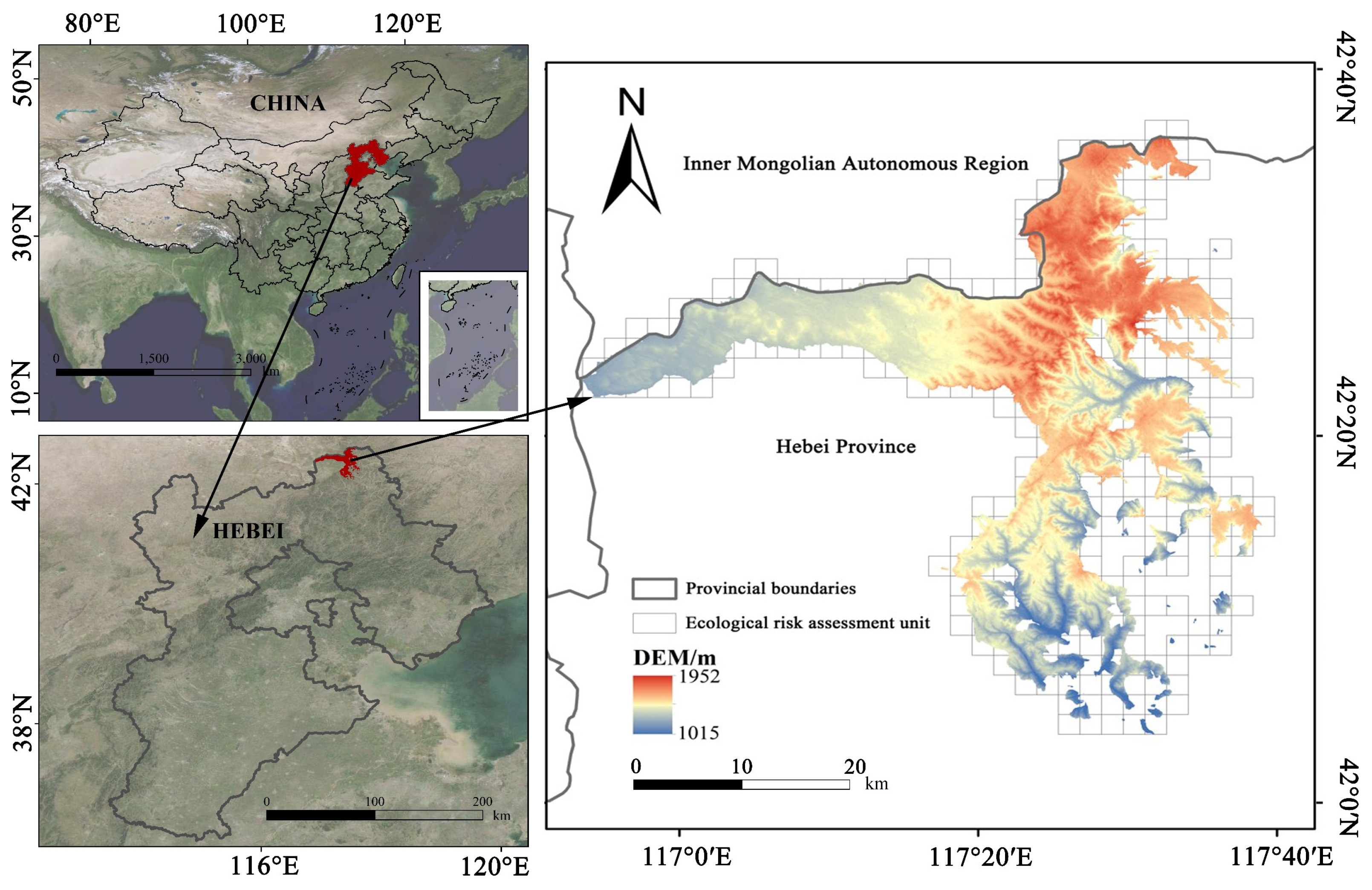
2.1. Study Area

The Saihanba Mechanical Forest Farm is located in the semi-arid and semi-humid zone (Figure 1), which is positioned at the intersection of the Yinshan Mountains, the Daxing’an Mountains, and the Hunshandake Sandy Land. It falls within the transitional area both below and above the dam, marking the juncture of forest–grassland and arid–semi-arid regions. The topography is characterized by a north-to-south slope, creating a distinctive landform with higher elevations in the north and lower elevations in the south. The altitude ranges from 1010 to 1940 m, with an average annual temperature of −1.2 °C, an average annual sunshine duration of 2548.7 h, and an average annual precipitation of approximately 452.2 mm, primarily concentrated in the months of June to September.
The Saihanba Mechanical Forest Farm has strategically embraced the concept of the “four banks” of forests as a pivotal strategy for advancing high-quality development in forestry and grassland management. This approach serves as a valuable model for fostering integrated protection and systematic governance across diverse ecosystems, including mountains, rivers, forests, farmland, lakes, and grasslands. Leveraging the synergistic benefits of the forest “four reservoirs” concept, the farm aims to maximize high-level advantages, thereby promoting development and enhancing the well-being of the local population. Presently, the predominant forest resources consist of artificially cultivated pure forests, with key tree species including Larix principis-rupprechtii, Pinus sylvestris var. mongolica, Picea asperata, Betula platyphylla, among others.
In history, the Saihanba area was a hunting paddock of the Qing government, with a good natural environment and many trees. Due to a lack of finance, a large number of trees were cut down and the forest coverage rate decreased sharply. Subsequently, the Japanese invasion of China caused a serious fire, and the destruction of forest resources became more serious. After the founding of the People’s Republic of China, it began to pay attention to ecological construction.
Currently, the total value of Saihanba Forest Farm forest resources has reached CNY 20.2 billion, the total value of forest resources is about USD 2.8 billion, driving the local social income of more than USD 80 million every year. Saihanba will build a global ecological civilization and green development demonstration zone in the next, striving to create higher social and economic benefits.
The establishment of Saihanba Mechanical Forest Farm has alleviated the ecological crisis in the Beijing–Tianjin–Hebei region and even the entire north region of China. But while the external crisis has been alleviated, problems such as single tree species and fragmentation of patches have appeared inside the forest farm, and the landscape risk is unknown.

2.2. Data Source

The Landsat remote sensing images from 1987, 1997, 2001, 2013, and 2020 used in this paper were acquired from the United States Geological Survey (https://glovis.usgs.gov/). Analysis of the images was conducted using ENVI 5.1 software. The support vector machine classification method was applied to categorized the preprocessed images. To align with the research objectives, the images were segmented into five distinct classes: forest, grassland, wetland, sandy land, and construction land (Figure 2). To ensure the accuracy of the classification, a confusion matrix was established, and verification results indicated that the kappa coefficients for the interpreted land use maps during the five periods consistently exceeded 0.76, meeting the accuracy standards for medium-resolution remote sensing images.
Precipitation, soil type, DEM, vegetation cover grade, air temperature, slope aspect, slope, and subcompartment accumulation were selected from the second-class survey data of subcompartment in Saihanba Mechanical Forest Farm.

2.3. Methods

2.3.1. Analysis of Temporal and Spatial Changes in Land Use and Vegetation Cover

The SVM classification method revealed significant landscape type changes in 1987–2020. Therefore, the transfer matrix method was used to explore the amount of exchanges of each landscape type over the entire period of 1987–2020, and the NDVI was calculated to see if there was a trend of decreasing vegetation cover classes.

Normalized Vegetation Index

The normalized difference vegetation index ( N D V I ) is extensively used in the research and application of vegetation cover changes, and has a linear relationship with the vegetation distribution density [45,46,47]. Its formula is:
N D V I = ( N I R R E D ) / ( N I R + R E D )
The notation used in this context defines NIR as the reflection value in the near-infrared band, and RED as the reflection value in the red band. Specifically, in Landsat 2 TM images, these correspond to band 6 for NIR and band 5 for RED. In Landsat 5–8 TM images, the relevant bands are band 4 for NIR and band 3 for RED.

Transfer Matrix Method

The transition matrix model serves to elucidate the initial probability of various stages and the transitions between these stages, thereby allowing the determination of change trends before and after different periods. The formula for this model is:
S i j = S 11 S 12 S 1 n S 21 S 22 S 2 n S n 1 S n 2 S n n
where S reflects the coverage area for each vegetation grade; n reflects the number of vegetation cover grade types; i and j reflect the vegetation cover grade types at the initiation and commencement of the study period, respectively.

2.3.2. Landscape Ecological Risk Analysis

Division of Landscape Ecological Risk Units

In this study, according to the national grid GIS standard “Geographical Grid” (GB12409-2009) and related research, the grid size was determined based on 2–5 times the average patch area in the study area [48]. The ArcGIS fishnet creation function was employed to partition the study area into ecological risk units of 2 km × 2 km, and these fishnets were subsequently segmented to generate a total of 382 ecological risk units. Utilizing landscape ecological risk value assignment, the semi-variation function within the Kriging interpolation method was applied for spherical fitting, yielding the landscape ecological risk level map across different periods.

Construction of Landscape Ecological Risk Index

The landscape index, through the comprehensive analysis of multiple indices, enables a quantitative reflection of the landscape pattern and its dynamic changes. In this study, landscape fragmentation, dispersion, dominance, vulnerability, and disturbance were designated as landscape ecological risk indices.
Calculating the landscape disturbance index through the landscape fragmentation index, landscape separation index, and landscape dominance index can reflect the complexity of spatial structure. The landscape vulnerability index reflects the ecological sensitivity of the study area. The higher the vulnerability, the worse the resistance to interference. The landscape loss index is calculated by combining the landscape disturbance index and the landscape vulnerability index. According to the results, the landscape ecological risk index was then calculated (Table 1).

2.3.3. Spatial Autocorrelation Analysis

Spatial autocorrelation analysis was employed to unveil the spatial correlation characteristics of a specific attribute unit and its neighboring attribute units based on eigenvalues [52]. It was used to measure the distribution characteristics and interrelationships of spatial risk data.

Global Autocorrelation

The global Moran’s I index was utilized to assess the spatial correlation of attribute values within a unit across the entire study area.
G l o b a l   M o r a n s I = i = 1 n i = 1 m W i j x i x ¯ x j x ¯ S 2 i = 1 n j = 1 m W i j
S 2 = 1 n i = 1 n x i x 2
x ¯ = 1 n i = 1 n x i
where x i represents the observation value of the i -th area, n is the number of grids, and W i j is a binary adjacency space weight matrix, which is used to represent the adjacency relationship of spatial objects. When the area i and the area j are adjacent, W i j = 1; when the area i and the area j are not adjacent, W i j = 0.

Local Autocorrelation

The local Moran’s I index was employed to reflect the correlation between the attribute value of a unit and the adjacent spatial units.
L o c a l   M o r a n s I i = x i x ¯ m j = 1 n W i j ( x i x ¯ )
m = j = 1 j i n x j 2 / n 1 x 2
The Moran’s I value ranges from −1 to 1. A positive Moran’s I (>0) suggests a positive correlation in the study area, indicating that the attribute values of the study units are convergent. Conversely, a negative Moran’s I (<0) signifies a negative correlation and a dispersed distribution of attribute values. When Moran’s I equals 0, it indicates the absence of spatial correlation.

2.3.4. Geographical Detector

The geographical detector model, optimized for parameters, encompasses four functions: factor detector, interaction detector, ecological detector, and risk detector, each capable of handling various types of variables [53,54]. It can be used to test the stratified heterogeneity of a single factor; it can also be used to detect a possible causal relationship between two factors by testing the coupling of their spatial distributions.
In this study, the factor detector, interaction detector, and ecological detector were employed to investigate the comprehensive influence of diverse risk factors in the forest landscape on the risk level of the Saihanba forest landscape in 2020.

Factor Detector

Factor detector was used to measure the impact strength of each risk factor on the risk of forest landscapes. The detection method is:
q = 1 1 N σ 2 h = 1 L N h σ h 2
where q is the influence of a certain factor on the spatial distribution of landscape ecological risk, the value range is [−1, 1]; L is the partition number; h is composed of N h units; N σ and N are the unit numbers of layer h and the whole region, respectively.

Ecological Detector

The ecological detector reflects whether the risk factors have significant differences in the spatial distribution of landscape ecological risk, and it is measured by the F test. The formula is as follows:
F = N n = 1 ( N n = 2 1 )   σ n = 1 2 N n = 2 ( N n = 1 1 ) σ n = 2 2
where N n = 1 , N n = 2 represents the sample size in the two risk factor partitions, and the null hypothesis σ n = 1 2 = σ n = 2 2 . Rejecting the null hypothesis at the chosen significance level signifies the presence of significant differences between the two factors influencing the spatial distribution of landscape ecological risk.

Interaction Detector

In assessing whether an interaction exists among various risk factors impacting the spatial distribution of landscape ecological risk, we ascertained whether the two factors operate independently or interactively influence the spatial distribution of landscape ecological risk. This determination is achieved through a comparative analysis of the interactions between the two risk factors, encompassing the following five relationships:
If q (A∩B) < Min (q (A), q (B)), it means that the nonlinearity of the two factors is weakened;
If Min (q (A), q (B)) <q (A∩B) < Max (q (A), q (B)), it means that the single-factor nonlinearity is weakened;
If q (A∩B) > Max (q (A), q (B)), it means two-factor enhancement;
If q (A∩B) = q (A) + q (B), it means that the two factors are independent of each other;
If q (A∩B) > q (A) + q (B), it means two-factor nonlinear enhancement.

3. Research Results and Analysis

3.1. Analysis of Landscape Dynamic Change

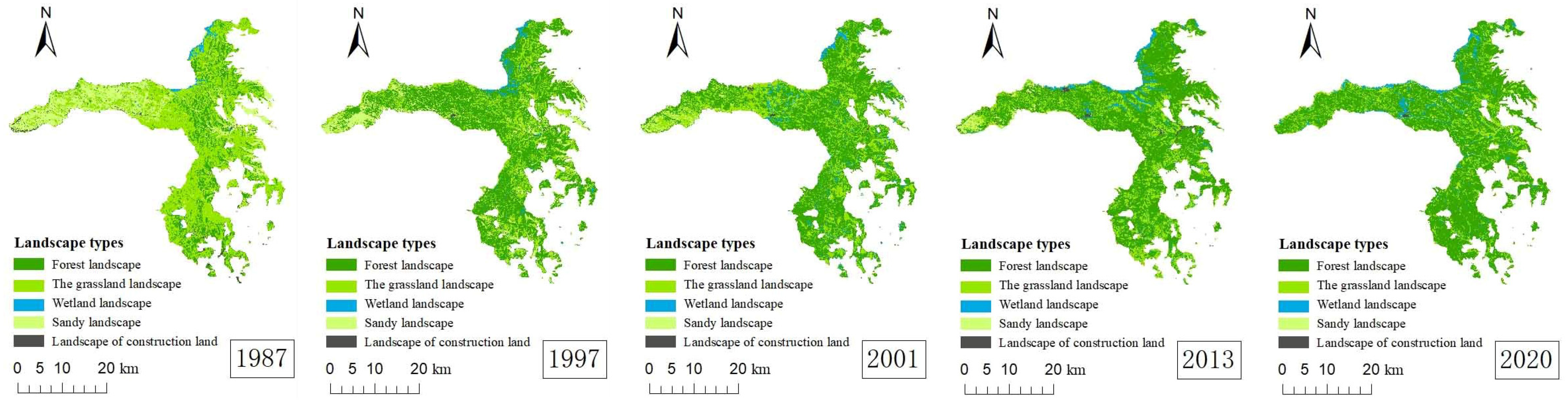
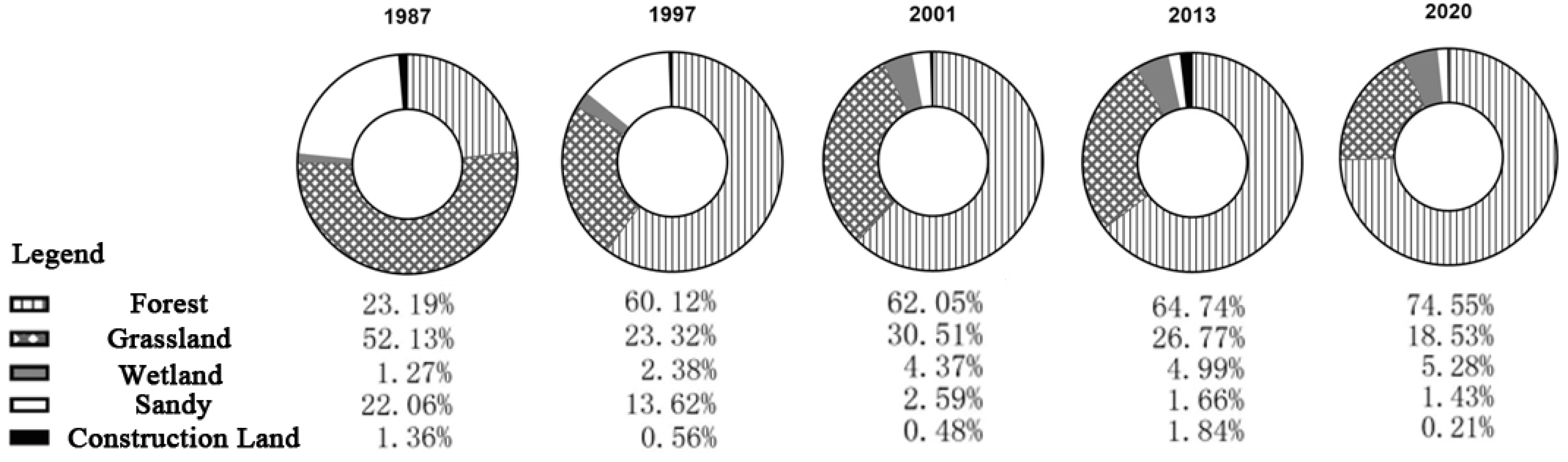
3.1.1. Analysis of Structural Changes of Landscape Types

Figure 3 illustrates the evolution of landscape types in Saihanba from 1987 to 2020. Over this period, the forest and wetland areas had significant growth, while grassland, sandy land, and construction land areas declined. Particularly noteworthy is the significant expansion of woodland, registering a remarkable increase of 479.06 km2, constituting approximately half of the total study area and elevating its proportion from 23.19% to 74.55%. The wetland area experienced a significant increase of 37.39 km2, more than threefold compared to 1987, with its proportion in the total study area rising from 1.27% to 5.28%. In contrast, the areas of grassland, sandy land, and construction land decreased by 313.33 km2, 192.37 km2, and 10.75 km2, respectively. Consequently, their proportional representation decreased from 52.13%, 22.06%, 1.36% to 18.53%, 1.43%, and 0.21%, respectively.

3.1.2. Landscape Type Structure Transfer Analysis

Changes in the landscape type transition matrix in the overall period from 1987 to 2020 are shown in Table 2. In general, forests and wetlands were the transfer-in types, and grassland, sandy land, and construction land were the transfer-out types. A large amount of grassland, sandy land, and construction land were transferred to forests, while a small amount of grassland and sandy land were transferred to wetland. In addition, there were different degrees of transformation among the various landscape types.
Vegetation cover changes over the entire period 1987–2020 are shown in Table 3. The extremely high vegetation cover grade was the type of transfer-in, and the area was greatly increased. The vegetation cover grade was transferred out to different degrees. Among them, the extremely low, and low and medium coverage was greatly reduced, and the overall vegetation cover grade significantly improved.

3.2. Analysis of Temporal and Spatial Changes in Landscape Risk

To investigate the spatial and temporal distribution characteristics of landscape ecological risk in Saihanba, the ecological risk index (ERI) for each landscape risk evaluation unit served as its attribute value. The spatial and temporal distribution of landscape ecological risk in Saihanba was determined using the ordinary Kriging interpolation tool in ArcGIS. Considering the specific conditions of the study area and the ERI across five phases, the natural breakpoint method was applied to categorize the study area into five landscape ecological risk levels: high-risk area (ERI > 0.29), mid-high-risk area (0.29 < ERI ≤ 0.26), medium-risk area (0.26 < ERI ≤ 0.23), mid-low-risk area (0.23 < ERI ≤ 0.21), and low-risk area (ERI ≤ 0.21). The results are presented in Figure 4 and Table 4.
Overall (Figure 4 and Figure 5, Table 4), the landscape stability of Saihanba has been continuously improved, accompanied by a noticeable decline in landscape ecological risk. The expanse of low-risk areas has consistently expanded, while the areas of other risk grades have experienced a continual reduction over time. Examining the changes in landscape ecological risk areas across all levels in Saihanba, it is evident that in 1987, the medium-risk area constituted the largest portion, with medium-risk, mid-high-risk, and high-risk areas collectively accounting for 72.30% of the total area. The overall risk was relatively high, particularly in the central-south and northeast regions, which displayed elevated risk values. By 1997, with the exception of low-risk levels, the area of other risk levels was significantly reduced, with low-risk areas accounting for 88.55 percent of the total area, signifying a significant risk reduction. However, the risk shifted from the central-south and northeast to the west and northwest spatially. The western region was characterized by sandy land dominance, while the northwestern region was characterized by wetlands, resulting in relatively high landscape vulnerability. In 2001, the areas of both low-risk and high-risk areas experienced slight increases. The high-risk area expanded from the northwest to the north along the border line, and the regions in the south-midwest transformed from low-risk to high-risk areas. In 2013, the low- and mid-low-risk areas witnessed upward trends, increasing by 49.2 km2 and 3.53 km2, respectively. Spatially, the risk values in the western and northwestern regions exhibited effective improvement, while certain areas in the central and eastern regions showed enhanced risk. These areas contained farmlands, impacting the landscape’s stability, displaying a high degree of vulnerability and significant plaque fragmentation. By 2020, low-risk areas continued to grow, while other risk areas demonstrated a diminishing trend, indicating a considerable improvement in ecological risk across the study area.

3.3. Spatial Autocorrelation Analysis of Landscape Ecological Risk

3.3.1. Landscape Type Structure Transfer Analysis

Utilizing the temporal and spatial distribution data of landscape ecological risk in Saihanba from 1987 to 2020, a Moran’s I scatter plot was generated. This case is depicted in Figure 6. The landscape ecological risk values of Saihanba were 0.177, 0.120, 0.127, 0.205, and 0.072 in 1987, 1997, 2001, 2013, 2020 and 2020. Notably, the Moran’s I value peaked in 2013, signifying a relatively strong spatial agglomeration effect for landscape ecological risk. It suggests that the regional landscape ecological risk values have a significant impact on the adjacent regional landscape ecological risk values. Conversely, the Moran’s I value hit its lowest point in 1997, indicating a comparatively weak agglomeration effect. In comparison to other years, the regional landscape ecological risk value had a slightly less pronounced impact on the adjacent regional landscape ecology during this period.

3.3.2. Local Correlation Analysis

Conducting a more in-depth examination of the local spatial correlation of landscape ecological risk in Saihanba, we derived a local spatial autocorrelation clustering map (refer to Figure 7). Overall, the distribution of high-value areas in each year closely aligned with the spatial distribution observed in Kriging interpolation. In 1987, high-value areas were concentrated along the southwest boundary of the study area. The patches in this area were highly fragmented, mainly forests, with a small amount of wetland, and the degree of landscape loss was high. In contrast, low-value areas were scattered. By 1997, high-value areas shifted to the western region, with a minor distribution in the northwest. The high-value areas in the western region were dominated by sandy land, grasslands and forests. Some areas witnessed the transformation of grassland and sandy land into forests, resulting in patch fragmentation and diminished landscape stability. Sporadic low-value areas in the northeast, primarily composed of wetlands with high landscape vulnerability, were evident. In 1987, low-value areas were dispersed within high-value areas, suggesting that during this period, patch fragmentation underwent timely adjustments. Landscape patches in this area transitioned from low-fragility to high-fragility, reducing landscape loss. In 2001, high-value areas showed no significant change, but there was a noteworthy increase in low-value areas, particularly concentrated in the northeast. In 2013, the risk in high-value areas in the west and northwest became less prominent, with high-value areas exhibiting a sporadic distribution. In 2020, certain high-value areas increased in the central and western regions, predominantly composed of wetlands with relatively high landscape vulnerability. Concurrently, the distribution of low-value areas in the south transformed from being insignificant to concentrated.

3.4. Ecological Risk Analysis of Forest Landscape in 2020

3.4.1. Local Correlation Analysis

According to the forest landscape analysis of Saihanba in 2020 (Figure 8), the areas with mid-high and high-risk levels were primarily distributed in southern and northern regions, and the medium-risk regions were clustered in the southwestern, central, and western regions. From the global autocorrelation analysis, the ecological risk of forest landscape presented a clustering effect in space. Regarding local autocorrelation analysis, the spatial distribution of high-value areas and forest landscape risk levels was relatively consistent. The main distribution landscapes were large-scale larch forests and birch forests. The spatial distribution of Pinus sylvestris forests was primarily medium risk. The risk of the rest of the landscape is favorable.

3.4.2. Forest Landscape Risk Ecological Detection Results

Nine risk factors were classified using the natural breakpoint method, and the classification results are shown in the figure (Figure 9).

Risk Factor Detection and Analysis

The detection results, presented in the table, indicate that the impact strength of the risk factor on landscape ecological risk increases with a larger q value. Among the nine risk factors, the intensity of detection results of forest landscape risk factors in Saihanba is as follows: soil type > precipitation > forest landscape type > air temperature > slope > DEM > slope aspect > subcompartment volume > vegetation cover grade. From the degree of significance of differences, soil type, precipitation, forest landscape type, air temperature, slope, DEM, and slope aspect have extremely significant differences in forest landscape risk, other factors have no significant difference on forest landscape risk, as shown in Table 5.

Analysis of Risk Ecology Detection

The determination of significant differences in the spatial distribution of risk factors influencing landscape ecological risks is accomplished through ecological detection. The test, conducted at a significance level of 0.05, assesses whether two factors exhibit significant differences in influencing the distribution of landscape ecological risks. The detection results, depicted in Figure 10, reveal notable distinctions in landscape ecological risk between soil type and other factors, as well as between precipitation and other factors. Additionally, there are significant differences in other factors, such as DEM, vegetation cover grade, slope aspect, subcompartment volume and forest landscape type;slope, air temperature, and vegetation cover grade, which together play a role in landscape ecological risk. However, there is no significant difference between other factors and landscape ecological risk, indicating that each risk factor has a lesser impact on forest landscape ecology in the study area, maintaining overall stability.

Risk Interaction Detection Analysis

Using the method of interactive detection, we can detect whether different risk factors have interactive effects on the spatial distribution of landscape ecological risks (Table 6). The interaction between the two factors was significantly higher than the single factor alone. Among them, the nonlinear enhancement effect was more significant than the double-factor enhancement. It also showed that there was no independent effect between the factors, indicating the impact of forest landscape ecological changes was the result of multiple factors. Forest landscape type and precipitation, forest landscape type and soil type, precipitation and soil type, slope and soil type have double-factor enhancement effects, and the other factors are nonlinear enhancement effects, which alone affect the spatial distribution of ecological risks.

4. Discussion

4.1. Landscape Pattern and Spatial Scale Change in Landscape Ecological Risk

In this research, we used NDVI and the transition matrix method, and found that the landscape pattern of Saihanba has undergone substantial changes from 1987 to 2020, and the vegetation cover grade area has increased significantly. Among diverse landscape types, there was an upward trajectory in the area of forests and wetlands, while the areas of grassland, sandy land, and construction land exhibited a declining trend.
In 1987, the overall risk was relatively high, and the risk was significantly reduced in 1997. This was related to the decrease in grassland and sand and the substantial increase in forest area from 1987 to 1997. Before 1987, China began extensive afforestation: as an important strategic location in China, a large number of forests were planted in Saihanba. Until 1997, tree growth resulted in increased crown density, so that through remote sensing imagery we found that the landscape changed markedly during this period, and this change was mainly due to the trees that were planted on grasslands and sandy land. Based on the spatial correlation analysis, the changes to landscape risk within the five periods all showed a positive correlation trend. This was consistent with the results of many scholars that changes in land use have a significant effects on landscape ecological risks [1,55,56,57].

4.2. Evaluation Method of Landscape Ecological Risk Index

The assessment of regional landscape ecological risk primarily relies on landscape pattern index evaluation [58,59] and ecosystem service value [60,61]. Given the significant changes in the landscape pattern over more than 40 years in the study area, the variation in the landscape ecological risk index is primarily attributed to alterations in the landscape pattern. The landscape ecological risk index exhibited a continuous decrease from 1987 to 2020. Notably, from 2013 to 2020, the high-risk area of landscape ecology remained relatively stable with no noticeable transfers, indicating an inward contraction trend in the high-risk area. However, diverse quantitative methods yielded different outcomes for the landscape ecological risk assessment, and the subjective nature of landscape vulnerability classification impacted the spatial distribution of landscape ecological risk. Consequently, the assessment of landscape ecological risk in this study remains relatively one-sided. Moving forward, it is imperative to further account for the influence of additional factors on landscape ecological risk.
Building on the evaluation of the landscape ecological risk index from 1987 to 2020, a more focused investigation into the risk of forest landscapes in 2020 was conducted. Through a comprehensive analysis of landscape ecological risk in the study area, the vulnerability of the forest landscape was determined based on the risk level associated with each forest landscape, combined with the expert consultation method. The findings revealed that mid-high and high-risk areas were dispersed in the south, northeast, and central parts of the study area, primarily characterized by extensive larch forests and birch forests. This study suggests the need to adjust stand structures within a reasonable range in these areas.

4.3. Analysis of Forest Landscape Risk Drivers and Suggestions for Future Development

Addressing the ecological risk status of the forest landscape in 2020, the geographical detector method was employed to delve into its governing factors. Recognizing that the internal structure of the forest landscape and various geographical factors exert a substantial impact on landscape risk, nine factors with a significant influence on the Saihanba forest landscape were chosen based on the management status of the Saihanba Mechanical Forest Farm. The study revealed that the forest landscape type poses the greatest risk to landscape ecology, aligning with the findings of numerous experts. Simultaneously, this observation is connected to the classification method of landscape vulnerability. Currently, research on landscape ecological risk predominantly focuses on river basins and coastlines, leaving a research gap in the context of forest landscapes [62]. Therefore, building upon the landscape risk in the study area, this study compared the risk levels of each forest landscape and classified landscape vulnerability based on expert advice.
Soil type, precipitation, forest landscape type, temperature, slope, DEM, and slope direction have a significant impact on forest landscape ecological risk. Among these factors, there are significant differences in soil type and precipitation compared to other factors. Hence, this area should be designated as a pivotal zone for risk prevention to avert an upward trend in risk. Analyzing the factors that have a pronounced impact on the Saihanba Mechanical Forest Farm, including landscape type, slope, slope direction, precipitation, vegetation cover grade, and subcompartment volume, reveals that, apart from fixed geographical factors (slope, slope direction, precipitation), the vegetation cover grade has reached an optimal level, with low-value areas sparsely distributed, mainly found in water areas and construction land. Subcompartment volume is related to the forest landscape type and forest management. Therefore, formulating a reasonable forest management plan and gradually adjusting the forest landscape type, specifically the stand structure, is imperative. Currently, the stand structure is monotonous, necessitating the introduction of diverse tree species. Simultaneously, adhering to the principle of suitable tree species and updating the forest patch configuration, as suggested by this study, not only contributes to mitigating the risk of the forest landscape but also holds significant ecological importance for forest carbon storage and enhancing forest site quality.
Utilizing the landscape ecological risk index and spatial autocorrelation analysis, this study assessed the ecological risk pattern of the Saihanba Mechanical Forest Farm from the viewpoint of landscape spatial structure. Additionally, a geographic detector was employed to analyze risk-driving factors. From the results, the effect of multi-factor combination is not simply one-plus-one, but far greater than the single factor, so it should be fully considered in the management and development of forest farms. Since the establishment of Saihanba, extensive tree planting efforts have significantly improved the ecological environment, resulting in substantial changes to the landscape pattern. Given that landscape pattern alterations inherently impact ecosystem functions, utilizing landscape pattern indices to investigate the ecological risk pattern is both feasible and effective. Consequently, it is recommended that the Saihanba Mechanical Forest Farm maintains and adjusts its existing landscape structure and addresses high-risk areas in alignment with its specific conditions. At the same time, to pay attention to the diversity of forest structure and its spatiotemporal variation characteristics is necessary [62]. The enhancement of the landscape integration pattern should prioritize natural factors. During resource development, adhering to the principle of ecological priority is crucial. While safeguarding river waters and promoting forestry development, it is imperative to regulate the uncontrolled development of local tourism. Zoning management, aligned with the current state, should be implemented, coupled with the establishment of an effective ecological compensation system.

5. Conclusions

In this study, the landscape ecological risk of the Saihanba Mechanical Forest Farm was comprehensively evaluated from four aspects: land use change and transfer, spatial-temporal distribution, spatial correlation of landscape ecological risk, and risk factor detection. The results are shown as follows:
(1)
Between 1987 and 2020, the Saihanba forest landscape area increased, along with a corresponding rise in wetland coverage. Conversely, grassland, sandy land, and construction land areas experienced a decrease. The forest landscape emerged as the predominant type in Saihanba, exerting a significant influence on the overall landscape pattern change.
(2)
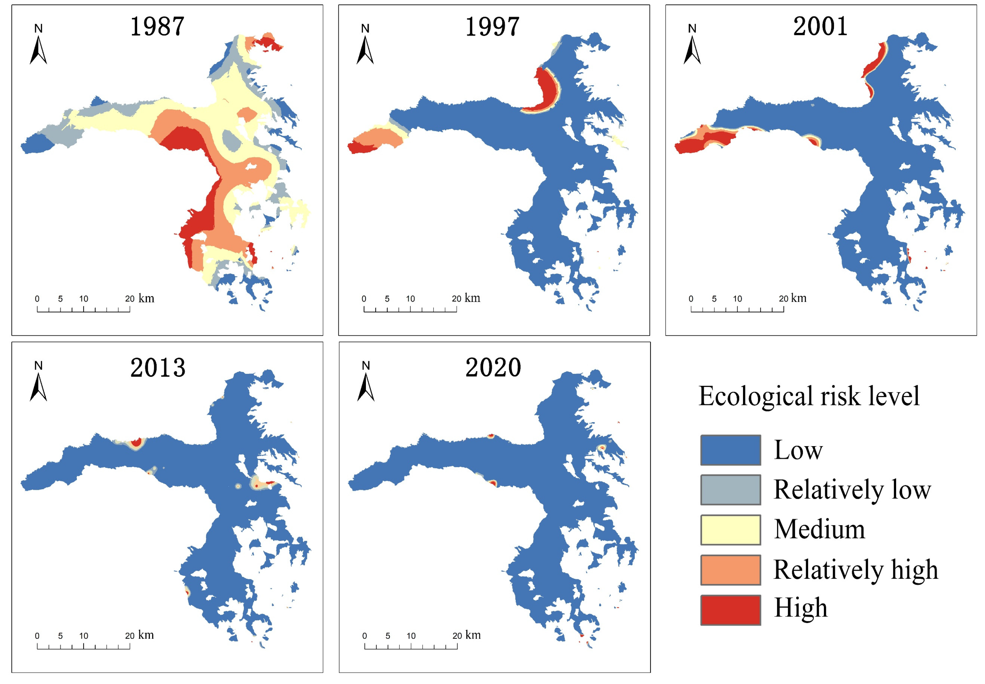
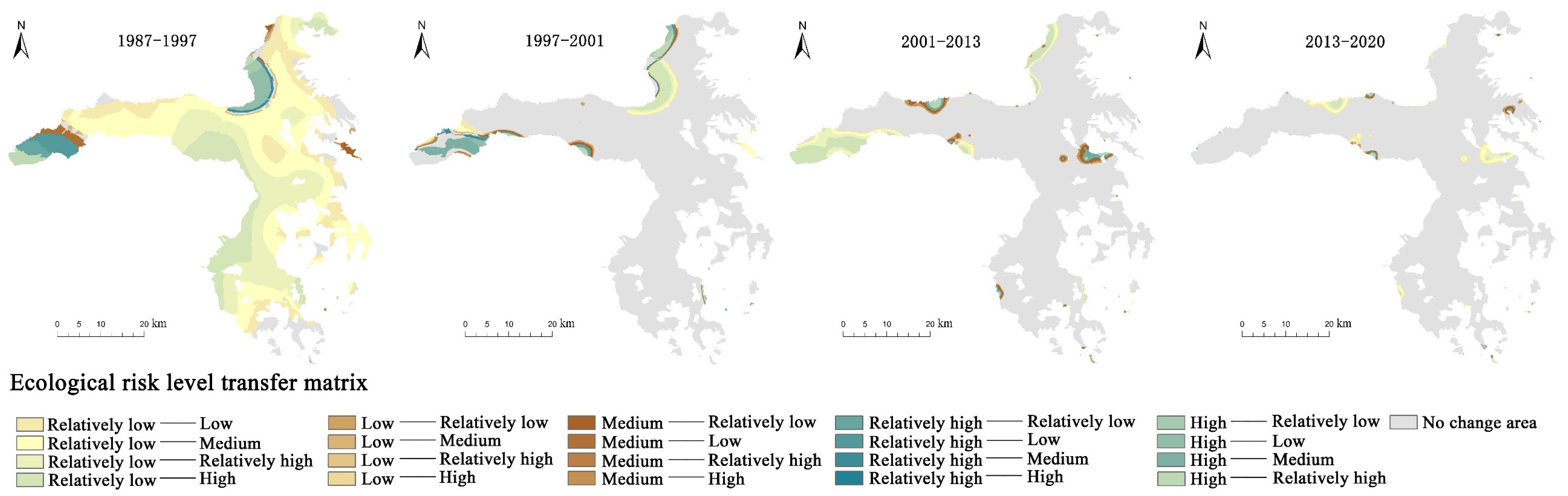
Between 1987 and 2020, the Saihanba area experienced a continuous reduction in the extent of medium-, mid-high-, and high-risk levels, coupled with a significant increase in the low-risk area. Spatially, the overall risk level was relatively high in 1987. In the period from 1997 to 2001, the risk level demonstrated a significant decrease, but there was a spatial shift in the risk areas. During this time, the high-risk area was limited to the border between the west and northwest, indicating an overall decreasing trend of landscape ecological risk. From 2013 to 2020, the landscape predominantly comprised low-risk areas. The medium-, mid-high-, and high-risk areas were confined to a small, aggregated distribution, without outward spread. The overall landscape ecological risk tended to stabilize during this period.
(3)
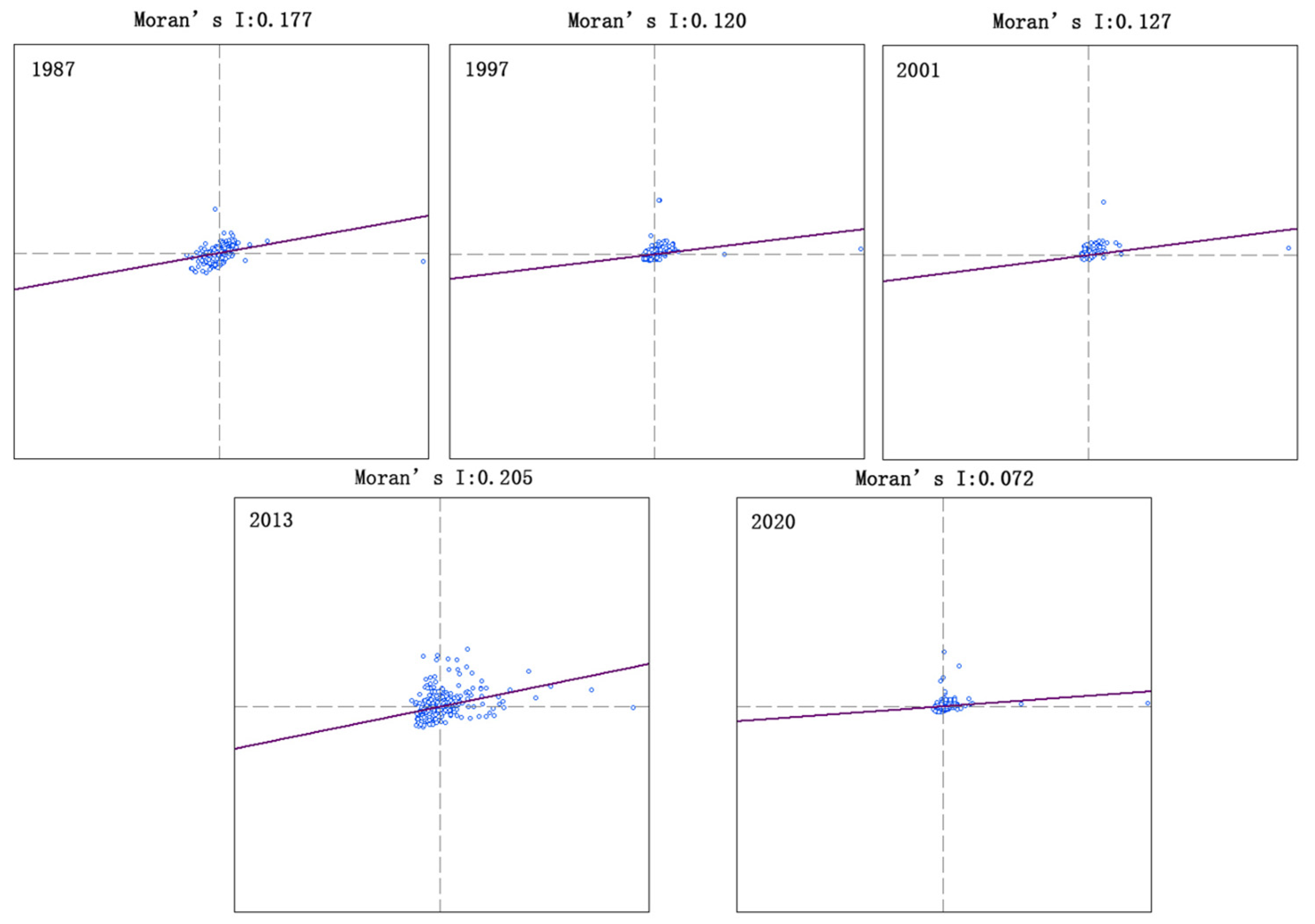
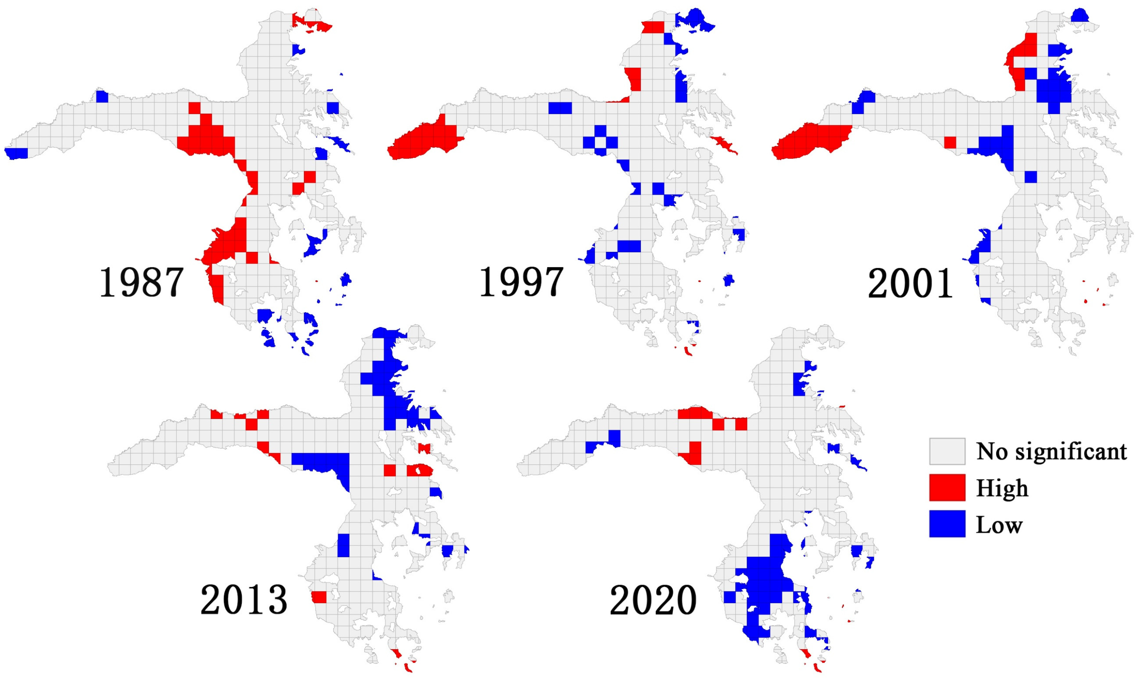
Throughout the study period, the global autocorrelation Moran’s I values of the watershed were 0.177, 0.120, 0.127, 0.205 and 0.072 respectively. The landscape ecological risks were positively correlated and tended to be clustered in spatial distribution. The landscape ecological risk level showed greater alignment with the high and low values of the local autocorrelation pattern.
(4)
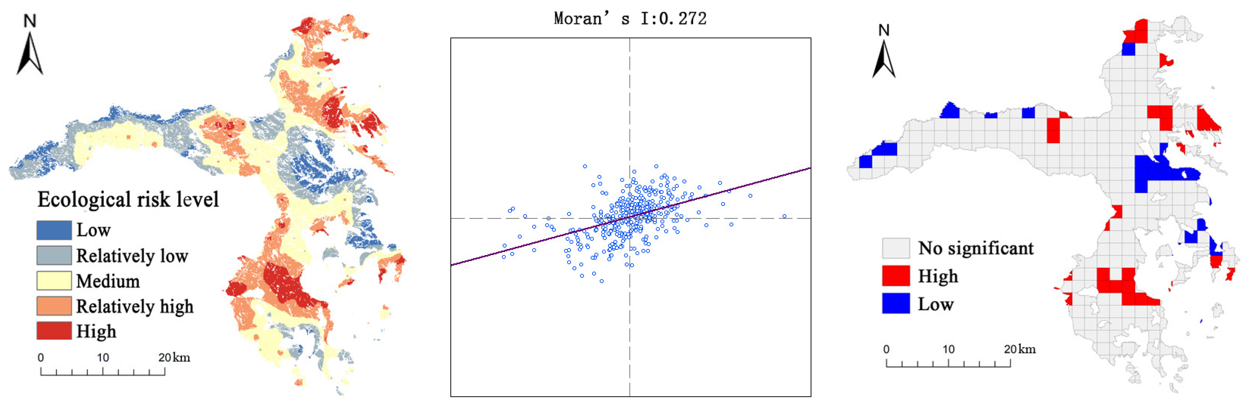
Analyzing the landscape ecological risk distribution map in 2020 enabled a detailed examination of the risk associated with various forest landscapes. The vulnerability was classified based on the risk value of each forest landscape. It was observed that the southern and northern regions exhibited higher risk levels, predominantly characterized by pure forests. Mitigating the risk of the forest landscape in these areas requires measures to enhance the stand structure.
(5)
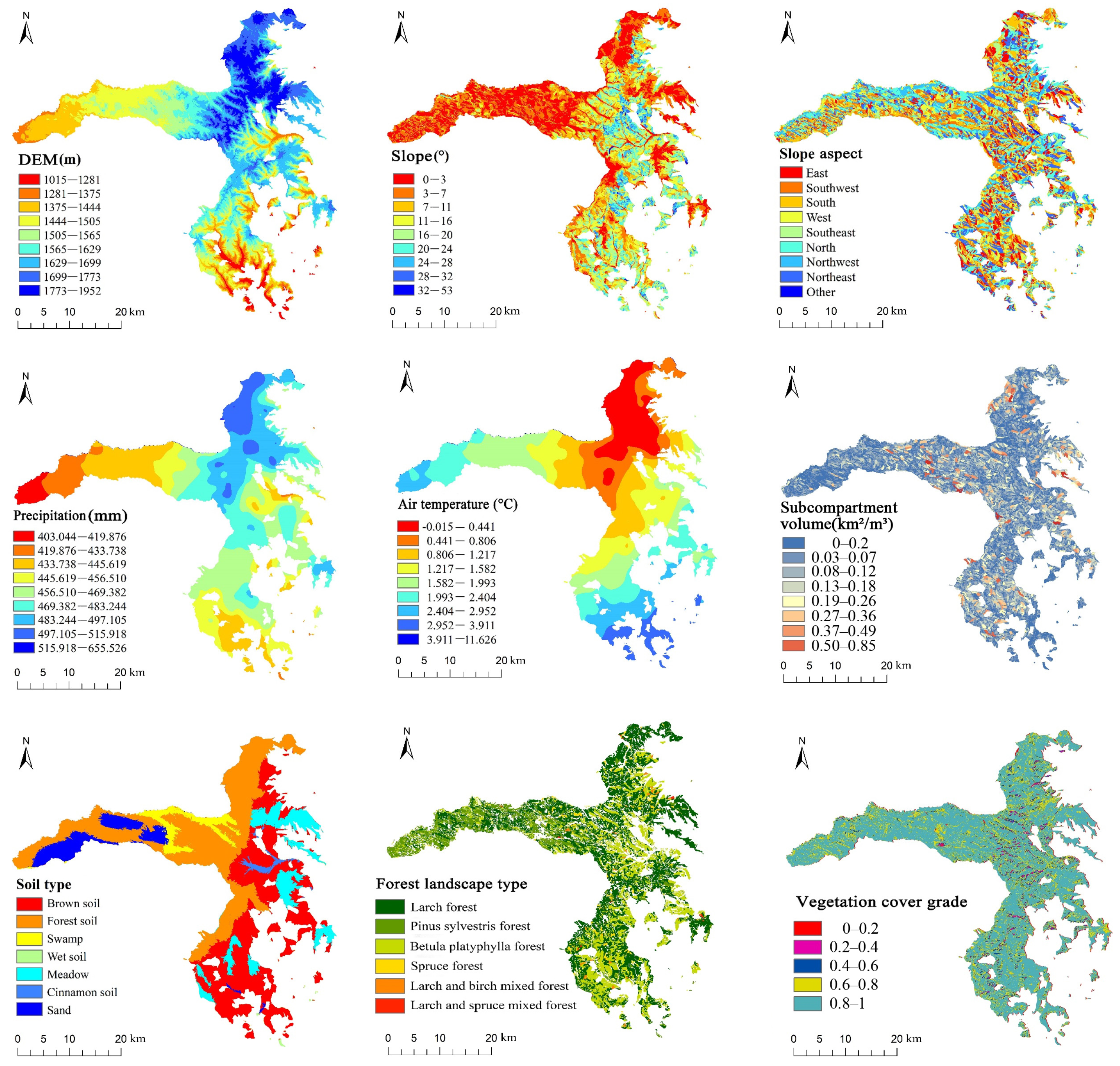
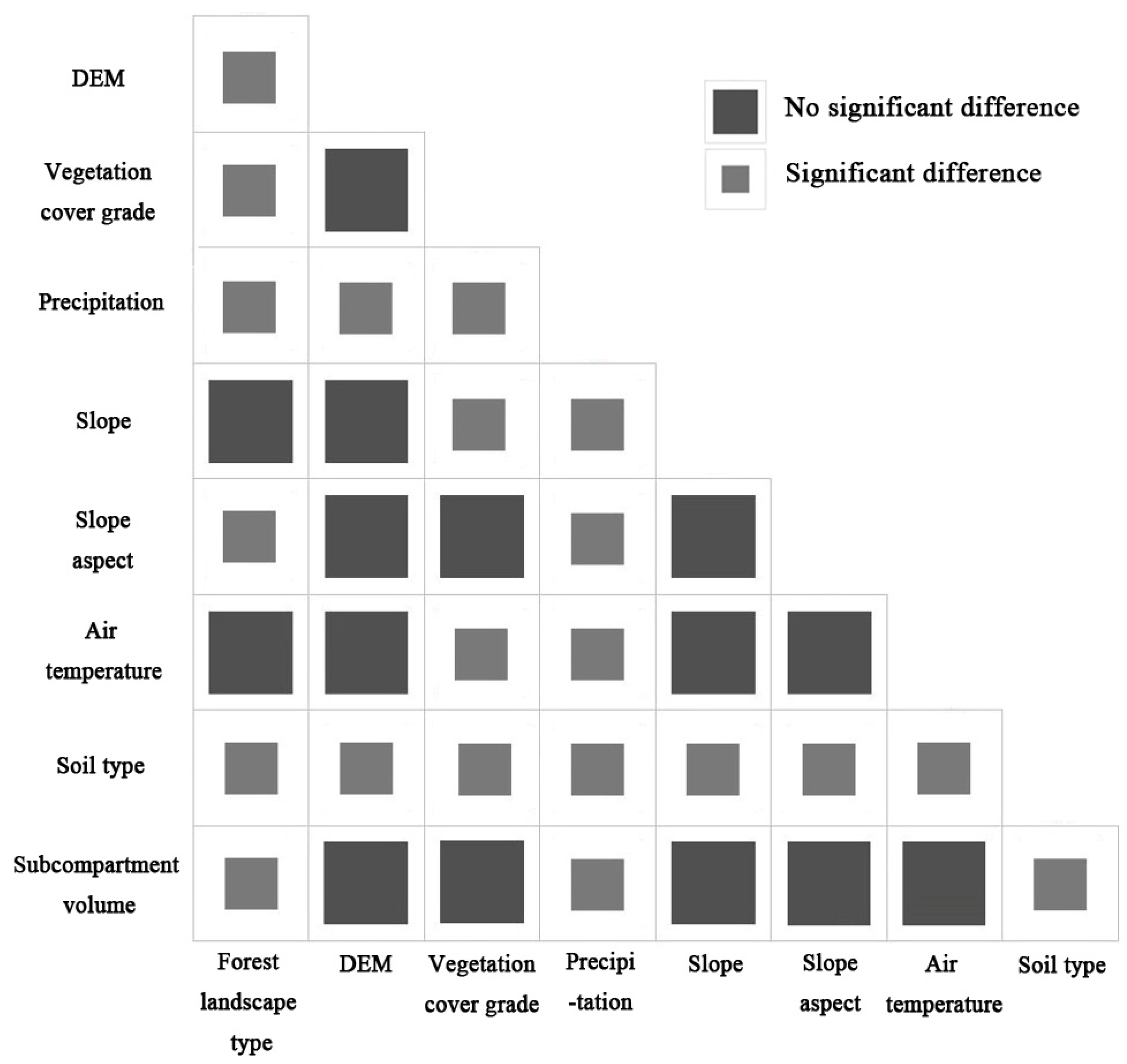
In the analysis of regional risk factors for each landscape risk level in 2020, it was determined that soil type, precipitation, forest landscape type, temperature, slope, DEM, and slope aspect exerted significant influence on forest landscape ecology risk. Among these factors, soil type had the most substantial impact, and its interaction with precipitation, as well as with other factors, played a crucial role. Notably, the interactions between forest landscape type and precipitation, forest landscape type and soil type, precipitation and soil type, and slope and soil type were considerably stronger than the influence of each factor in isolation.

Author Contributions

J.K. and W.L. conceived and designed this research, collected the data, processed the satellite images, and performed the experiments; J.K. conducted the analysis and drafted the manuscript; J.Y. and Y.Q. revised the manuscript. All authors have read and agreed to the published version of the manuscript.

Funding

This research was funded by the Key technological innovation and demonstration projects of Forestry and Grassland Bureau of Hebei Province (2406101), the National Natural Science Foundation of China (32201556), the Key R&D Program Projects of Hebei Province 22326807D, the National Natural Science Foundation of China (31700561), the Asia Pacific Network for Sustainable Forest Management and Rehabilitation (2021SP2-CHN),and the Fundamental Research Funds for the Hebei Provincial Universities (KY2022046).

Data Availability Statement

Restrictions apply to the availability of these data. Landsat remote sensing images are available from the United States Geological Survey (https://glovis.usgs.gov/). Non-remote sensing data was obtained from the Saihanba Mechanical Forest Farm and are available from the authors with the permission of the Saihanba Mechanical Forest Farm.

Acknowledgments

We thank the United States Geological Survey for sharing Landsat remote sensing images(https://glovis.usgs.gov/). We gratefully acknowledge the data support provided by Saihanba Forest Farm for sharing the second-class inventory data.

Conflicts of Interest

The authors declare no conflicts of interest.

References

  1. Zhang, S.; Shao, H.; Li, X.; Xian, W.; Shao, Q.; Yin, Z.; Lai, F.; Qi, J. Spatiotemporal Dynamics of Ecological Security Pattern of Urban Agglomerations in Yangtze River Delta Based on LUCC Simulation. Remote Sens. 2022, 14, 296. [Google Scholar] [CrossRef]
  2. Ding, Y.; Feng, H.; Zou, B.; Ye, S. Contribution Isolation of LUCC Impact on Regional PM2.5 Air Pollution: Implications for Sustainable Land and Environment Management. Front. Environ. Sci. 2022, 10, 825732. [Google Scholar] [CrossRef]
  3. Chu, X.-L.; Lu, Z.; Wei, D.; Lei, G.-P. Effects of land use/cover change (LUCC) on the spatiotemporal variability of precipitation and temperature in the Songnen Plain, China. J. Integr. Agric. 2022, 21, 235–248. [Google Scholar] [CrossRef]
  4. Zhang, L.; Jiang, Y.; Yang, M.; Wang, H.; Dong, N.; Wang, H.; Liu, X.; Chen, L.; Liu, K. Quantifying the Impacts of Land Use and Cover Change (LUCC) and Climate Change on Discharge and Sediment Load in the Hunhe River Basin, Liaoning Province, Northeast China. Water 2022, 14, 737. [Google Scholar] [CrossRef]
  5. Jiang, P.; Cheng, L.; Li, M.; Zhao, R.; Duan, Y. Impacts of LUCC on soil properties in the riparian zones of desert oasis with remote sensing data: A case study of the middle Heihe River basin, China. Sci. Total Environ. 2015, 506–507, 259–271. [Google Scholar] [CrossRef]
  6. Özşahin, E.; Eroğlu, I. Soil Erosion Risk Assessment due to Land Use/Cover Changes (LUCC) in Bulgaria from 1990 to 2015. Alinteri J. Agric. Sci. 2019, 34, 1–8. [Google Scholar] [CrossRef]
  7. Bi, W.; Weng, B.; Yuan, Z.; Ye, M.; Zhang, C.; Zhao, Y.; Yan, D.; Xu, T. Evolution Characteristics of Surface Water Quality Due to Climate Change and LUCC under Scenario Simulations: A Case Study in the Luanhe River Basin. Int. J. Environ. Res. Public Health 2018, 15, 1724. [Google Scholar] [CrossRef]
  8. Dou, X.; Huang, W.; Yi, Q.; Liu, X.; Zuo, H.; Li, M.; Li, Z. Impacts of LUCC and climate change on runoff in Lancang River Basin. Acta Ecol. Sin. 2019, 39, 4687–4696. [Google Scholar] [CrossRef]
  9. Zhang, X.; Shao, Y. LUCC impact on water quality change in Xingyun Lake basin. E3S Web Conf. 2020, 198, 04025. [Google Scholar] [CrossRef]
  10. Meng, L.; Dong, J. LUCC and Ecosystem Service Value Assessment for Wetlands: A Case Study in Nansi Lake, China. Water 2019, 11, 1597. [Google Scholar] [CrossRef]
  11. Zhou, R.; Lin, M.; Gong, J.; Wu, Z. Spatiotemporal heterogeneity and influencing mechanism of ecosystem services in the Pearl River Delta from the perspective of LUCC. J. Geogr. Sci. 2019, 29, 831–845. [Google Scholar] [CrossRef]
  12. Ji, Y.; Bai, Z.; Hui, J. Landscape Ecological Risk Assessment Based on LUCC—A Case Study of Chaoyang County, China. Forests 2021, 12, 1157. [Google Scholar] [CrossRef]
  13. Luo, K.; Zhang, X. Increasing urban flood risk in China over recent 40 years induced by LUCC. Landsc. Urban Plan. 2021, 219, 104317. [Google Scholar] [CrossRef]
  14. Dale, V.H.; Brown, S.; Haeuber, R.A.; Hobbs, N.T.; Huntly, N.; Naiman, R.J.; Riebsame, W.E.; Turner, M.G.; Valone, T.J. Ecological Principles and Guidelines for Managing the Use of Land. Ecol. Appl. 2000, 10, 639–670. [Google Scholar] [CrossRef]
  15. Walker, R.; Landis, W.; Brown, P. Developing A Regional Ecological Risk Assessment: A Case Study of a Tasmanian Agricultural Catchment. Hum. Ecol. Risk Assess. Int. J. 2001, 7, 417–439. [Google Scholar] [CrossRef]
  16. Ayre, K.K.; Landis, W.G. A Bayesian Approach to Landscape Ecological Risk Assessment Applied to the Upper Grande Ronde Watershed, Oregon. Hum. Ecol. Risk Assess. Int. J. 2012, 18, 946–970. [Google Scholar] [CrossRef]
  17. Yanes, A.; Botero, C.M.; Arrizabalaga, M.; Vásquez, J.G. Methodological proposal for ecological risk assessment of the coastal zone of Antioquia, Colombia. Ecol. Eng. 2019, 130, 242–251. [Google Scholar] [CrossRef]
  18. Mocaer, A.; Guillou, E.; Chouinard, O. The social construction of coastal risks in two different cultural contexts: A study of marine erosion and flooding in France and Canada. Int. J. Disaster Risk Reduct. 2021, 66, 102635. [Google Scholar] [CrossRef]
  19. Qi, Y.; Yao, Z.; Ma, X.; Ding, X.; Shangguan, K.; Zhang, M.; Xu, N. Ecological risk assessment for organophosphate esters in the surface water from the Bohai Sea of China using multimodal species sensitivity distributions. Sci. Total Environ. 2022, 820, 153172. [Google Scholar] [CrossRef]
  20. Nishitha, D.; Amrish, V.N.; Arun, K.; Warrier, A.K.; Udayashankar, H.N.; Balakrishna, K. Study of trace metal contamination and ecological risk assessment in the sediments of a tropical river estuary, Southwestern India. Environ. Monit. Assess. 2022, 194, 94. [Google Scholar] [CrossRef]
  21. Yousefpour, R.; Gray, D.R. Managing forest risks in uncertain times of climate change. Ann. For. Sci. 2022, 79, 16. [Google Scholar] [CrossRef]
  22. Heinonen, T.; Pukkala, T.; Ikonen, V.-P.; Peltola, H.; Gregow, H.; Venäläinen, A. Consideration of strong winds, their directional distribution and snow loading in wind risk assessment related to landscape level forest planning. For. Ecol. Manag. 2011, 261, 710–719. [Google Scholar] [CrossRef]
  23. Pricope, N.G.; Hidalgo, C.; Pippin, J.S.; Evans, J.M. Shifting landscapes of risk: Quantifying pluvial flood vulnerability beyond the regulated floodplain. J. Environ. Manag. 2022, 304, 114221. [Google Scholar] [CrossRef] [PubMed]
  24. Akçakaya, H. Linking population-level risk assessment with landscape and habitat models. Sci. Total Environ. 2001, 274, 283–291. [Google Scholar] [CrossRef] [PubMed]
  25. Qin, H.; Brenkert-Smith, H.; Sanders, C.; Vickery, J.; Bass, M. Explaining changes in perceived wildfire risk related to the mountain pine beetle outbreak in north central Colorado. Ecol. Indic. 2021, 130, 108080. [Google Scholar] [CrossRef]
  26. Naumann, T.; Bento, C.P.; Wittmann, A.; Gandrass, J.; Tang, J.; Zhen, X.; Liu, L.; Ebinghaus, R. Occurrence and ecological risk assessment of neonicotinoids and related insecticides in the Bohai Sea and its surrounding rivers, China. Water Res. 2021, 209, 117912. [Google Scholar] [CrossRef]
  27. Hossain, S.; Ramirez, J.A.; Haisch, T.; Speranza, C.I.; Martius, O.; Mayer, H.; Keiler, M. A coupled human and landscape conceptual model of risk and resilience in Swiss Alpine communities. Sci. Total Environ. 2020, 730, 138322. [Google Scholar] [CrossRef] [PubMed]
  28. Wang, Q.; Zhang, P.; Chang, Y.; Li, G.; Chen, Z.; Zhang, X.; Xing, G.; Lu, R.; Li, M.; Zhou, Z. Landscape pattern evolution and ecological risk assessment of the Yellow River Basin based on optimal scale. Ecol. Indic. 2024, 158, 111381. [Google Scholar] [CrossRef]
  29. Kong, J.; Ma, T.; Cao, X.; Li, W.; Zhu, F.; He, H.; Sun, C.; Yang, S.; Li, S.; Xian, Q. Occurrence, partition behavior, source and ecological risk assessment of nitro-PAHs in the sediment and water of Taige Canal, China. J. Environ. Sci. 2022, 124, 782–793. [Google Scholar] [CrossRef]
  30. Zhao, Y.; Li, J.; Qi, Y.; Guan, X.; Zhao, C.; Wang, H.; Zhu, S.; Fu, G.; Zhu, J.; He, J. Distribution, sources, and ecological risk assessment of polycyclic aromatic hydrocarbons (PAHs) in the tidal creek water of coastal tidal flats in the Yellow River Delta, China. Mar. Pollut. Bull. 2021, 173, 113110. [Google Scholar] [CrossRef]
  31. Hasan, M.; al Ahmed, A.; Islam, A.; Rahman, M. Heavy metal pollution and ecological risk assessment in the surface water from a marine protected area, Swatch of No Ground, north-western part of the Bay of Bengal. Reg. Stud. Mar. Sci. 2022, 52, 102278. [Google Scholar] [CrossRef]
  32. Xinge, W.; Jianchao, X.; Dongyang, Y.; Tian, C. Spatial Differentiation of Rural Touristization and Its Determinants in China: A Geo-Detector-Based Case Study of Yesanpo Scenic Area. J. Resour. Ecol. 2016, 7, 464–471. [Google Scholar] [CrossRef]
  33. Qian, X.; Wang, D.; Nie, R. Assessing urbanization efficiency and its influencing factors in China based on Super-SBM and geographical detector models. Environ. Sci. Pollut. Res. 2021, 28, 31312–31326. [Google Scholar] [CrossRef]
  34. Ge, K.; Zou, S.; Lu, X.; Ke, S.; Chen, D.; Liu, Z. Dynamic Evolution and the Mechanism behind the Coupling Coordination Relationship between Industrial Integration and Urban Land-Use Efficiency: A Case Study of the Yangtze River Economic Zone in China. Land 2022, 11, 261. [Google Scholar] [CrossRef]
  35. Xu, X.; Zhao, Y.; Zhang, X.; Xia, S. Identifying the Impacts of Social, Economic, and Environmental Factors on Population Aging in the Yangtze River Delta Using the Geographical Detector Technique. Sustainability 2018, 10, 1528. [Google Scholar] [CrossRef]
  36. Wang, J.; Ma, J.J.; Liu, J.; Zeng, D.D.; Song, C.; Cao, Z. Prevalence and Risk Factors of Comorbidities among Hypertensive Patients in China. Int. J. Med. Sci. 2017, 14, 201–212. [Google Scholar] [CrossRef]
  37. Liu, X.; Wang, H.; Wang, X.; Bai, M.; He, D. Driving factors and their interactions of carabid beetle distribution based on the geographical detector method. Ecol. Indic. 2021, 133, 108393. [Google Scholar] [CrossRef]
  38. Qiao, P.; Lei, M.; Guo, G.; Yang, J.; Zhou, X.; Chen, T. Quantitative Analysis of the Factors Influencing Soil Heavy Metal Lateral Migration in Rainfalls Based on Geographical Detector Software: A Case Study in Huanjiang County, China. Sustainability 2017, 9, 1227. [Google Scholar] [CrossRef]
  39. Dong, S.; Pan, Y.; Guo, H.; Gao, B.; Li, M. Identifying Influencing Factors of Agricultural Soil Heavy Metals Using a Geographical Detector: A Case Study in Shunyi District, China. Land 2021, 10, 1010. [Google Scholar] [CrossRef]
  40. Ju, H.; Zhang, Z.; Zuo, L.; Wang, J.; Zhang, S.; Wang, X.; Zhao, X. Driving forces and their interactions of built-up land expansion based on the geographical detector—A case study of Beijing, China. Int. J. Geogr. Inf. Sci. 2016, 30, 2188–2207. [Google Scholar] [CrossRef]
  41. Wang, Y.; Wang, S.; Li, G.; Zhang, H.; Jin, L.; Su, Y.; Wu, K. Identifying the determinants of housing prices in China using spatial regression and the geographical detector technique. Appl. Geogr. 2017, 79, 26–36. [Google Scholar] [CrossRef]
  42. Fan, Z.; Duan, J.; Lu, Y.; Zou, W.; Lan, W. A geographical detector study on factors influencing urban park use in Nanjing, China. Urban For. Urban Green. 2021, 59, 126996. [Google Scholar] [CrossRef]
  43. Xu, J.; Liu, H.; Li, B.; Gao, X.; Nie, P.; Sun, C.; Jin, Z.; Zhai, D. Identifying factors that affect environmental air quality using geographical detectors in the NKEFAs of China. Front. Earth Sci. 2021, 16, 499–512. [Google Scholar] [CrossRef]
  44. Li, M.; Abuduwaili, J.; Liu, W.; Feng, S.; Saparov, G.; Ma, L. Application of geographical detector and geographically weighted regression for assessing landscape ecological risk in the Irtysh River Basin, Central Asia. Ecol. Indic. 2024, 158, 111540. [Google Scholar] [CrossRef]
  45. Dong, Y.; Yin, D.; Li, X.; Huang, J.; Su, W.; Li, X.; Wang, H. Spatial–Temporal Evolution of Vegetation NDVI in Association with Climatic, Environmental and Anthropogenic Factors in the Loess Plateau, China during 2000–2015: Quantitative Analysis Based on Geographical Detector Model. Remote Sens. 2021, 13, 4380. [Google Scholar] [CrossRef]
  46. Liu, Y.; Tian, J.; Liu, R.; Ding, L. Influences of Climate Change and Human Activities on NDVI Changes in China. Remote Sens. 2021, 13, 4326. [Google Scholar] [CrossRef]
  47. Ogou, F.K.; Ojeh, V.N.; Naabil, E.; Mbah, C.I. Hydro-climatic and Water Availability Changes and its Relationship with NDVI in Northern Sub-Saharan Africa. Earth Syst. Environ. 2021, 6, 681–696. [Google Scholar] [CrossRef]
  48. Rangel-Buitrago, N.; Neal, W.J.; de Jonge, V.N. Risk assessment as tool for coastal erosion management. Ocean Coast. Manag. 2020, 186, 105099. [Google Scholar] [CrossRef]
  49. Ju, H.; Niu, C.; Zhang, S.; Jiang, W.; Zhang, Z.; Zhang, X.; Yang, Z.; Cui, Y. Spatiotemporal patterns and modifiable areal unit problems of the landscape ecological risk in coastal areas: A case study of the Shandong Peninsula, China. J. Clean. Prod. 2021, 310, 127522. [Google Scholar] [CrossRef]
  50. Ai, J.; Yu, K.; Zeng, Z.; Yang, L.; Liu, Y.; Liu, J. Assessing the dynamic landscape ecological risk and its driving forces in an island city based on optimal spatial scales: Haitan Island, China. Ecol. Indic. 2022, 137, 108771. [Google Scholar] [CrossRef]
  51. Lv, L.; Zhang, J.; Sun, C.Z.; Wang, X.R.; Zheng, D.F. Landscape ecological risk assessment of Xi river Basin based on land-use change. Acta Ecol. Sin. 2018, 38, 5952–5960. [Google Scholar] [CrossRef]
  52. Luo, Y.; Yan, J.; Li, F.; Li, B. Spatial Autocorrelation of Martian Surface Temperature and Its Spatio-Temporal Relationships with Near-Surface Environmental Factors across China’s Tianwen-1 Landing Zone. Remote Sens. 2021, 13, 2206. [Google Scholar] [CrossRef]
  53. Song, Y.; Wang, J.; Ge, Y.; Xu, C. An optimal parameters-based geographical detector model enhances geographic characteristics of explanatory variables for spatial heterogeneity analysis: Cases with different types of spatial data. GISci. Remote Sens. 2020, 57, 593–610. [Google Scholar] [CrossRef]
  54. Gao, S.; Dong, G.; Jiang, X.; Nie, T.; Yin, H.; Guo, X. Quantification of Natural and Anthropogenic Driving Forces of Vegetation Changes in the Three-River Headwater Region during 1982–2015 Based on Geographical Detector Model. Remote Sens. 2021, 13, 4175. [Google Scholar] [CrossRef]
  55. Liu, D.; Chen, H.; Zhang, H.; Geng, T.; Shi, Q. Spatiotemporal Evolution of Landscape Ecological Risk Based on Geomorphological Regionalization during 1980–2017: A Case Study of Shaanxi Province, China. Sustainability 2020, 12, 941. [Google Scholar] [CrossRef]
  56. Han, N.; Yu, M.; Jia, P. Multi-Scenario Landscape Ecological Risk Simulation for Sustainable Development Goals: A Case Study on the Central Mountainous Area of Hainan Island. Int. J. Environ. Res. Public Health 2022, 19, 4030. [Google Scholar] [CrossRef] [PubMed]
  57. Zhang, S.; Zhong, Q.; Cheng, D.; Xu, C.; Chang, Y.; Lin, Y.; Li, B. Coupling Coordination Analysis and Prediction of Landscape Ecological Risks and Ecosystem Services in the Min River Basin. Land 2022, 11, 222. [Google Scholar] [CrossRef]
  58. Li, X.; Li, S.; Zhang, Y.; O’Connor, P.J.; Zhang, L.; Yan, J. Landscape Ecological Risk Assessment under Multiple Indicators. Land 2021, 10, 739. [Google Scholar] [CrossRef]
  59. Ma, H.; Yang, W.; Liu, Z.; Xu, R. Ecological risk assessment of ecological landscape pattern in Qin’an County. IOP Conf. Ser. Earth Environ. Sci. 2021, 675, 012006. [Google Scholar] [CrossRef]
  60. Jia, Y.; Tang, X.; Liu, W. Spatial–Temporal Evolution and Correlation Analysis of Ecosystem Service Value and Landscape Ecological Risk in Wuhu City. Sustainability 2020, 12, 2803. [Google Scholar] [CrossRef]
  61. Gong, J.; Cao, E.; Xie, Y.; Xu, C.; Li, H.; Yan, L. Integrating ecosystem services and landscape ecological risk into adaptive management: Insights from a western mountain-basin area, China. J. Environ. Manag. 2021, 281, 111817. [Google Scholar] [CrossRef] [PubMed]
  62. Mitchell, J.C.; Kashian, D.M.; Chen, X.; Cousins, S.; Flaspohler, D.; Gruner, D.S.; Johnson, J.S.; Surasinghe, T.D.; Zambrano, J.; Buma, B. Forest ecosystem properties emerge from interactions of structure and disturbance. Front. Ecol. Environ. 2023, 21, 14–23. [Google Scholar] [CrossRef]
Figure 1. Geographical location of Saihanba, China.
Forests 15 00700 g001
Figure 2. Landscape composition of Saihanba in different stages in 1987, 1997, 2001, 2013 and 2020.
Forests 15 00700 g002
Figure 3. Changes in the proportion of landscape types in 1987, 1997, 2001, 2013 and 2020.
Forests 15 00700 g003
Figure 4. Spatial distribution of landscape ecological risk levels in 1987, 1997, 2001, 2013 and 2020.
Forests 15 00700 g004
Figure 5. Spatial distribution of landscape ecological risk level transfer matrix in 1987, 1997, 2001, 2013, 2020.
Forests 15 00700 g005
Figure 6. The Moran scatter plot of landscape ecological risk in 1987, 1997, 2001, 2013, 2020.
Forests 15 00700 g006
Figure 7. Local spatial autocorrelation cluster map of landscape ecological risk in 1987, 1997, 2001, 2013, 2020.
Forests 15 00700 g007
Figure 8. Ecological risk distribution map within forest landscape, Moran scatter plot, spatial autocorrelation cluster map in Saihanba, 2020.
Forests 15 00700 g008
Figure 9. Spatial distribution of nine risk factors in forest landscapes.
Forests 15 00700 g009
Figure 10. Forest risk ecological detection results.
Forests 15 00700 g010
Table 1. Landscape ecological risk index calculation method.
IndexFormulaMeaning
Landscape Fragmentation Index C i C i = n i A i A i is the total area of the landscape type i ; A is the total area of the landscape; n i is the number of patches of the landscape type i ; Q i = the number of squares in which the patches i appear/the total number of squares; M i = the number of patches i /the total number of patches and; L i = the area of the patches i /the total area of the quadrat.
Landscape Separation Index N i N i = A 2 A i n i A
Landscape Dominance Index D i D i = Q i + M i 4 + L i 2
Landscape Disturbance Index E i E i = a C i + b N i + c D i a, b, and c represent the weights of fragmentation, separation, and dominance indices. Referring to relevant studies [49,50], the assigned values are determined to be 0.5, 0.3, and 0.2.
Landscape Vulnerability Index F i Expert consultation method and normalized treatmentReferring to relevant research [51], the vulnerability assignments of various landscapes in the study area were determined as follows: 5 for sandy land, 4 for wetland, 3 for grassland, 2 for forest, and 1 for construction land. Forest secondary classification landscape assignment: 5 for larch, 4 for sycamore pine and birch, 3 for spruce, 2 for mixed birch forest, and 1 for mixed forest of fallen clouds.
Landscape Loss Index R i R i = E i × F i A k i is the area of type i landscape in landscape ecological risk assessment unit k ; A k is the total area of landscape ecological risk assessment unit k ; E R i i is the landscape ecological risk index of landscape ecological risk assessment unit k, and its value is positively correlated with the degree of ecological risk.
Landscape Ecological Risk Index E R i i E R i i = i = 1 N A k i A k × R i
Table 2. Table of transfer area by landscape type, 1987–2020.
Matrix Transfer Area1987
UnitLandscape TypeForestGrasslandWetlandSandyConstruction Land
2020km2Forest169.73397.425.32119.685.76
km2Grassland31.0164.381.5568.425.84
km2wetland13.1416.664.9114.650.29
km2Sandy2.127.430.073.050.41
km2Construction land0.140.220.011.160.39
Table 3. Table of transfer area by vegetation cover, 1987–2020.
Matrix Transfer Area1987
UnitVegetation Cover GradeVery LowLowMiddleHighVery High
2020km2Very low0.01170.03780.05490.20250.9927
km2Low0.0630.10980.24840.777610.5687
km2Middle0.37980.78751.95845.387444.6472
km2High2.45886.27314.948132.1633120.6054
km2Very high19.520147.546185.0806155.8125379.8135
Table 4. Area table of change in ecological risk level in 1987, 1997, 2001, 2013 and 2020.
UnitEcological Risk LevelsLowRelatively LowMiddleRelatively HighHigh
km2198788.47170.24358.25211.10105.65
km21997827.1213.0519.3436.8637.04
km22001852.567.6610.3619.1343.69
km22013901.7611.199.76.803.95
km22020922.013.552.271.531.55
Table 5. Forest risk factor detection results.
Risk FactorSoil TypePrecipitationForest Landscape TypeAir TemperatureSlopeDEMSlope AspectSubcompartment VolumeVegetation Cover Grade
q statistic0.2280.1330.0760.0560.0560.0250.0160.0140.001
p value0.0000.0000.0000.0000.0000.0000.0000.0390.999
Table 6. Forest risk interaction detector results.
Forest Landscape TypeDEMVegetation Cover GradePrecipitationSlopeSlope AspectAir TemperatureSoil TypeSubcompartment Volume
Forest landscape type0.076
DEM0.136 #0.025
Vegetation cover grade0.081 #0.035 #0.001
Precipitation0.204 *0.203 #0.143 #0.133
Slope0.139 #0.178 #0.067 #0.241 #0.056
Slope aspect0.113 #0.077 #0.030 #0.182 #0.109 #0.016
Air temperature0.219 #0.160 #0.077 #0.461 #0.209 #0.124 #0.056
Soil type0.265 *0.313 #0.237 #0.345 *0.265 *0.253 #0.451 #0.228
Subcompartment volume0.096 #0.059 #0.021 #0.161 #0.089 #0.051 #0.100 #0.246 #0.014
Note: * denotes double factor enhancement, # denotes nonlinear enhancement.
Disclaimer/Publisher’s Note: The statements, opinions and data contained in all publications are solely those of the individual author(s) and contributor(s) and not of MDPI and/or the editor(s). MDPI and/or the editor(s) disclaim responsibility for any injury to people or property resulting from any ideas, methods, instructions or products referred to in the content.

