Environmental Response of Tree Species Distribution in Northeast China with the Joint Species Distribution Model

Abstract

The composition, distribution, and growth of native natural forests are important references for the restoration, structural adjustment, and close-to-nature transformation of artificial forests. The joint species distribution model is a powerful tool for analyzing community structure and interspecific relationships. It has been widely used in biogeography, community ecology, and animal ecology, but it has not been extended to natural forest conservation and restoration in China. Therefore, based on the 9th National Forest Inventory data in Jilin Province, combined with environmental factors and functional traits of tree species, this study adopted the joint species distribution model—including a model with all variables (model FULL), a model with environmental factors (model ENV), and a model with spatial factors (model SPACE)—to examine the distribution of multiple tree species. The results show that, in models FULL and ENV, the environmental factors explaining the model variation were ranked as follows, climate > site > soil. The explanatory power was as follows: model FULL (AUC = 0.8325, Tjur R² = 0.2326) > model ENV (AUC = 0.7664, Tjur R² = 0.1454) > model SPACE (AUC = 0.7297, Tjur R² = 0.1346). Tree species niches in model ENV were similar to those in model FULL. Compared to predictive power, we found that the information transmitted by environmental and spatial predictors overlaps, so the choice between model FULL and ENV should be based on the purpose of the model, rather than the difference in predictive ability. Both models can be used to study the adaptive distribution of multiple tree species in northeast China.

1. Introduction

Natural forests are the most stable, diverse, and structurally complex terrestrial ecosystems in nature; they play an irreplaceable role in responding to climate change, protecting biodiversity, and maintaining ecological balance [1,2]. China’s natural forest area reaches 138.68 million hectares, accounting for 63.55% of national forest area [3], making it a crucial strategic resource. The stock volume per unit area of China’s natural forests is 113.36 m³/ha, which is significantly lower compared to European countries with similar site conditions (where the stock volume exceeds 200 m³/ha) [4]. In July 2019, the General Office of the Central Committee of the Communist Party of China and the General Office of the State Council issued the “Natural Forest Conservation and Restoration System Scheme”, proposing the conservation and improvement of natural forest structure, focusing on cultivating native tree species, and enhancing forest quality. Therefore, protecting natural forest resources and enhancing the quality of natural forests has become a focus of forest management now and in the future.

The structure of stands, especially tree species composition, is a critical factor to consider in the restoration of natural forests. For a long time, the selection of target tree species and the determination of target forests in natural forest management have been mainly based on expert experience, lacking quantitative research. The composition, distribution, and growth conditions of tree species in virgin natural forests are important references for natural forest restoration, structural adjustment, and the near-natural management of plantations [5]. Currently, species distribution studies in Jilin Province are mainly limited to a few tree species and forest types, such as Betula platyphylla, Betula ermanii, Quercus mongolica, Larix gmelinii, and the broad-leaved forests of Pinus koraiensis [6,7,8]. Liu et al. conducted more systematic research using the MaxEnt model, but these studies have overlooked the interactions between species and cannot meet the needs of natural forest restoration and quality improvement in the region [9]. Therefore, it is necessary to adopt new methods to study the potential distribution suitability of the main forest types in northeast China’s natural forests.

Species in nature do not exist independently in the environment but coexist and interact within communities, also influenced by surrounding environmental factors [10]. Thus, species distribution is determined by both abiotic environmental factors (such as climate, soil, and topography) and biotic interactions between different species (such as predation, competition, and mutualism) [11,12]. With the development of computer technology and statistical methods, a species distribution modeling approach that combines environmental variables with interactions among multiple species (i.e., joint species distribution models) has been used in studies on the simulation and prediction of multi-species distributions [13,14,15]. Joint species distribution models, by using species correlation information and latent variables to predict missing environmental factors, can clearly select models and assess the model’s performance within the model framework, thereby simulating multi-species species–environment relationships and predicting the intensity and type of interactions between different species [16]. Not only does this enhance the interpretative power over ecological questions, but it also improves the flexibility and effectiveness of predicting species’ distribution suitability. Therefore, joint species distribution models are powerful tools for analyzing the structure of biological communities and interspecific relationships, widely applied in biogeography, community ecology, and animal ecology [17,18,19,20,21,22], but these models have not yet been widely applied in the conservation and restoration of China’s natural forests. Thus, understanding the distribution of multiple tree species and their interrelationships in natural forests has significant theoretical and practical significance for forest restoration.

Jilin province is located in the temperate zone, which has various types of natural forests, including coniferous forest, broad-leaved forest, mixed forest, etc. The distribution and combination of different tree species in the forest form a unique forest ecosystem. By studying the natural distribution of tree species, we can reveal the structure, function, and succession law of the forest ecosystem, and provide a scientific basis for the protection, restoration, and management of forest ecology. Therefore, the objectives of this study were as follows: (1) to construct a hierarchical model of species communities (HMSC) in combination with environmental factors and species functional traits for the distribution of multiple species; (2) to interpret tree species niches through the establishment of the best fitting joint species distribution model; and (3) to analyze effects of tree species traits and phylogeny on the HMSC model.

2. Materials and Methods

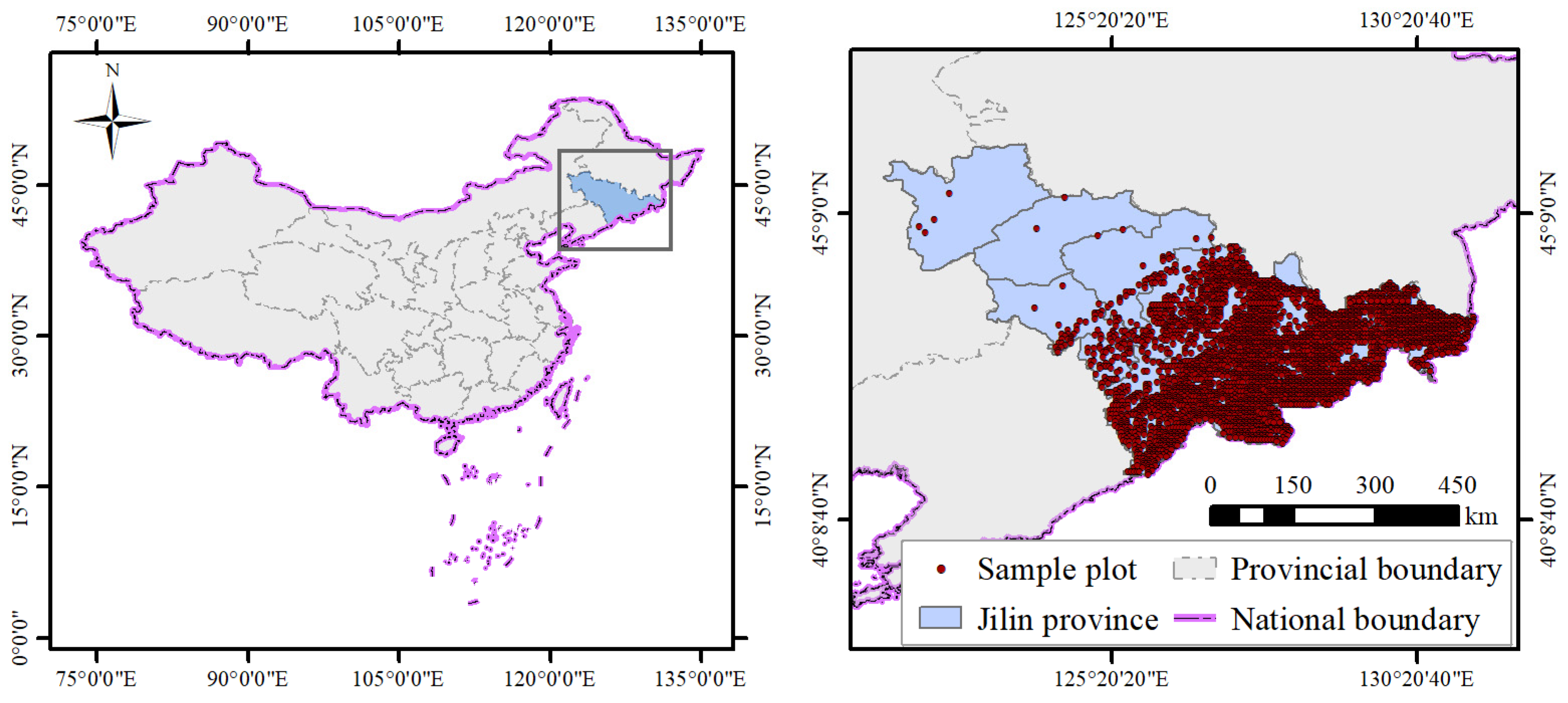
2.1. Study Area

The area involved in this study is the entirety of Jilin Province, located in the central part of northeast China, spanning from 121°38′ E to 131°19′ E longitude and 40°52′ N to 46°18′ N latitude. The terrain of Jilin Province exhibits a characteristic of being higher in the southeast and lower in the northwest, divided by the central Greater Khingan Range into eastern mountainous areas and central–western plains. There are 19 soil types within the province, with dark brown earth being predominant. The natural environment belongs to a temperate continental monsoon climate, with distinct seasonal changes and regional differences, forming a gradient of vegetation types from southeast to northwest characterized by moist, semi-moist, and semi-arid climates—from the moist forest climate in the east to the semi-moist forest-steppe climate in the center and the semi-arid steppe climate in the west. The average winter temperature does not exceed −11 °C, with summer temperatures generally above 23 °C. The annual average precipitation is between 400 and 600 mm, with annual average sunshine hours ranging from 2259 to 3016 h, and the frost-free period lasts between 100 and 160 days [9].

2.2. Data Collection

The data for the study area primarily revolve the ninth (2014) National Forest Inventory database in Jilin Province, encompassing five types of data needed: community data (species presence or abundance), environmental factors (site, soil, or climate), tree species functional traits (maximum tree height, wood density, and leaf area index, etc.), phylogenetic relationships of tree species, and plot spatial data.

2.2.1. Plot Data

The construction of the joint species distribution model primarily uses sample plot data on tree species composition by basal area, site factors, and latitude and longitude coordinates, focused on the central Changbai Mountain subregion. The species’ basal area compositions are extracted to form community data, with the basal area per hectare for each species calculated to form the community abundance data. Further, the basal area per hectare data are used to form presence–absence data for the community. Site factor data mainly include elevation, slope, aspect, position, soil (type and thickness), humus layer thickness, and litter thickness, from which site factor data in the environmental covariates can be obtained. Plot latitude and longitude coordinates form the spatial data. A total of 3309 permanent sample plot data points with each 600 m² from the ninth National Forest Inventory were collected for this study; their distributions are shown in Figure 1.

2.2.2. Climate Data

The climate data were sourced from the software ClimateAP V3.10, which is specifically designed for extracting climate factors in the East Asia–Pacific region (from https://web.climateap.net, accessed on 5 September 2023). ClimateAP allows users to extract and downscale gridded climate data to site-specific, scale-free climate data through a dynamic local downscaling method. ClimateAP calculates and exports many biologically relevant climate variables at monthly, seasonal, and annual timesteps [23]. The study area’s climate data were formed by registering and clipping with the basic geographic data of Jilin Province. For this study area, the climate data of 3309 sample plots were acquired, including 10 annual variables (MAT, MWMT, MCMT, TD, MAP, AHM, NFFD, EMT, Eref, and CMD), 8 seasonal variables (Tave_DJF, Tave_JJA, Tmax_DJF, Tmax_JJA, Tmin_DJF, Tmin_JJA, PPT_DJF, and PPT_JJA), and 48 monthly variables (Tave01–Tave12, Tmin01–Tmin12, Tmax01–Tmax12, and PPT01–PPT12). These abbreviations refer to Wang et al. [23].

2.2.3. Soil Data

Soil data were obtained from the SoilGrids system (version updated in June 2016), with a spatial resolution of 250 m. Based on the World Reference Base (WRB) and the United States Department of Agriculture (USDA) classification systems, totaling approximately 280 raster layers, the SoilGrids system provides global predictions of standard soil properties (organic carbon, bulk density, cation exchange capacity (CEC), pH value, soil structure ratio, and proportion of coarse fragments), bedrock depth, and soil type distributions at seven standard depths (0, 5, 15, 30, 60, 100, and 200 cm) [24]. Under the Open Database License (ODbL), the 250 m maps from SoilGrids V2.0 can be downloaded from www.SoilGrids.org (accessed on 15 September 2023). For this study area, 11 soil properties were acquired.

2.2.4. Tree Species Trait Factors Data

To assess the relationship between tree species niches and functional traits, it was necessary to collect functional trait data for the tree species appearing in the community data. Among the 3309 permanent sample plot data collected, a total of 75 tree species were involved. Due to the very low frequency of occurrence of many species, this study selected 31 tree species for further research, based on the criterion that the species appeared in more than 3% of all permanent sample plots. The species selected include the following: Pinus koraiensis Siebold et Zuccarini (sp1), Picea koraiensis Nakai (sp2), Picea jezoensis Carr. var. microsperma (Lindl.) Cheng et L.K.Fu (sp3), Abies nephrolepis (Trautv.) Maxim. (sp4), Abies holophylla Maxim. (sp5), Larix olgensis Henry (sp6), Pinus sylvestris Linn. var. mongolica Litv. (sp7), Quercus mongolica Fischer ex Ledebour (sp8), Tilia mandshurica Rmpr.et Maxim. (sp9), Tilia amurensis Rupr. (sp10), Ulmus davidiana Planch var. japonica (Rehd.) Nakai (sp11), Carpinus cordata Bl. (sp12), Ulmus laciniata (Trautv.) Mayr (sp13), Betula dahurica Pall. (sp14), Betula platyphylla Suk. (sp15), Betula costata Trautv. (sp16), Fraxinus mandschurica Rupr. (sp17), Juglans mandshurica Maxim. (sp18), Phellodendron amurense Rupr. (sp19), Acer mono Maxim. (sp20), Acer tegmentosum Maxim. (sp21), Acer mandshuricum Maxim. (sp22), Acer ukurunduense Trautv. et Mey. (sp23), Acer triflorum Komarov (sp24), Acer pseudo-sieboldianum (Pax) Komarov (sp25), Sorbus alnifolia (Sieb. et Zucc.) K. Koch (sp26), Fraxinus rhynchophylla Hance (sp27), Populus davidiana Dode (sp28), Populus ussuriensis Kom. (sp29), Populus simonii Carr. (sp30), and Salix matsudana Koidz. (sp31).

The trait factors for these tree species were obtained from the literature. Due to limitations in data acquisition, the trait factors compiled in this study include the following: wood density (WD), maximum height (H), leaf area (LA), specific leaf area (SLA), leaf dry matter density (LMA), leaf dry matter content (LDMC), leaf carbon concentration (Cmass), leaf nitrogen concentration (Nmass), leaf phosphorus concentration (Pmass), leaf potassium concentration (Kmass), area-based nitrogen content (Narea), area-based phosphorus content (Parea), and area-based potassium content (Karea).

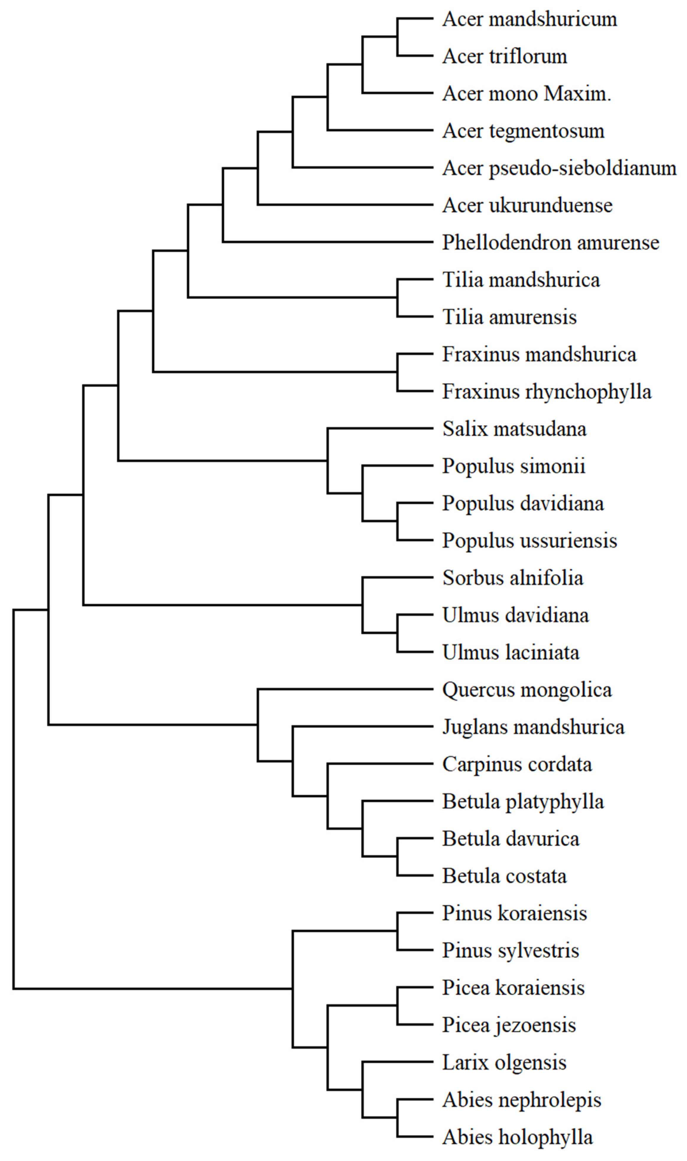
2.2.5. Tree Species Phylogenetic Data

To evaluate the extent to which tree species niches reflect phylogenetic relationships, phylogenetic data for the species were required. These data typically take the form of a phylogenetic tree, usually constructed by running genomic sequence data through phylogenetic analysis software and then generating a phylogenetic correlation matrix to describe the phylogenetic relationships among the species.

The procedure for generating the phylogenetic tree for the 31 tree species in this study began with obtaining protein molecular sequences for the species from the National Center for Biotechnology Information (www.ncbi.nlm.nih.gov, accessed on 12 December 2023). Due to the limitation of protein molecular sequence data for different organs of these 31 tree species, the chosen organ was the mature enzyme K (maturase K [chloroplast]) in tree leaves. Then, the Molecular Evolutionary Genetics Analysis software (MEGA_X_10.2.4) was used to perform phylogenetic analysis on the protein molecular sequence information of these tree species and generate usable phylogenetic tree files in NWK format. The finalized phylogenetic tree for these 31 tree species is shown in Figure 2.

2.3. Methods

A multivariate hierarchical generalized linear mixed model for 31 tree species in Jilin Province was constructed to study the relationship between environmental variables and the distribution of tree species, i.e., the niches of tree species, and further to elucidate the relationship between tree species niches, tree species traits, and phylogenetic trees.

2.3.1. Model Structure Setup and Fitting

Given that the structure of multiple tree species community data is of a presence–absence type, meaning the dependent variable is a 0–1 variable, the error distribution type of the model was chosen to use a probit link function, considering spatial random effects based on the geographic coordinates of the plots. To more comprehensively study the relationship between environmental covariates and spatial random effects, three types of model forms were considered. The first type is the full model (FULL), which includes both environmental covariates and spatial random effects of the plots. The second type is the environmental factor model (ENV), which includes only environmental covariates without the spatial random effects of the plots. The third type is the spatial factor model (SPACE), which includes only spatial random effects without environmental covariates. All three model structures introduced tree species traits and phylogenetic relationships.

After setting up the HMSC model structure, the parameter estimation phase requires fitting the data using the sampleMcmc function. Two MCMC chains were set, i.e., nChains = 2, with a sampling step size of 10 (thin = 10), and sampling 1000 times for each parameter (samples = 1000), discarding the first 5000 estimates (transient = 5000). Considering the spatial random effects and the sample size exceeding 1000, the computational complexity increased sharply, making the computation infeasible. Therefore, when dealing with the spatial structure, the Nearest Neighbor Gaussian Process (NNGP) was used. In this case, the parameter Method was set to “NNGP” and the corresponding parameter neighbors were set to the standard number, 10 according to the literature [25].

2.3.2. Variable Selection

In terms of variable selection, it is hypothesized that several typical predictive variables could influence the occurrence or abundance of species. Among these variables, some might have no impact, or some might be collinear with other predictive variables, thus carrying redundant information. Increasing the number of variables in the model raises the risk of over-parameterization, thereby increasing the risk of overfitting. Therefore, it is generally recommended to pre-select as few variables as possible, ensuring that the information content of these variables is maximized, and they are mutually independent [26]. In summary, at the first step, the most ecologically meaningful predictive variables should be selected, and predictive variables closely related to other predictors should be excluded to eliminate the multicollinearity among predictive variables.

In this study, environmental variables include 66 climatic factors (10 annual variables, 8 seasonal variables, and 48 monthly variables), 11 soil factors, and 7 site factors. Based on the principles analyzed above, using the results of previous work and considering ecological significance, along with the importance ranking in machine learning’s random forest algorithm, a selection is made. Liu found a significant response relationship between common tree species and forest types in Jilin Province and environmental factors, quantitatively measuring the impact of environmental variables on the distribution of tree species or forest types: climate > site > soil, indicating that climate is the most critical factor affecting vegetation distribution [4]. The specific environmental factors ranking (only top five selected) are as follows: the highest temperature of the hottest month, the average temperature of the hottest quarter, elevation, annual average temperature, and the average temperature of the coldest quarter. Soil factors have a smaller impact, but for conifer species, the significant ones are as follows: soil pH, bulk density, exchangeable hydrogen ions, exchangeable calcium ions, and available phosphorus. Machine learning with the data in the study is used to establish the relationship between tree species distribution and these environmental factors, employing the random forest algorithm. Based on the importance ranking, the top 10 influencing factors for each tree species are selected, and the frequency of each influencing factor is counted. The recommended results include climate factors NFFD, AHM, Eref, MCMT, TD, site factor ELE, soil factors bdod, soc, cfvo, and phh2o. Finally, to avoid variable collinearity, a correlation analysis is conducted for the shortlisted environmental variables, excluding variables with a correlation coefficient of 0.7 or above.

Therefore, from the environmental variables, seven climatic factors were selected: the average temperature of the hottest quarter (Tave_JJA), rainfall of the hottest quarter (PPT_JJA), number of frost-free days per year (NFFD), annual humidex (AHM), evapotranspiration (Eref), average temperature of the coldest month (MCMT), and the temperature difference between the hottest and coldest months (TD). One site factor was selected: elevation (ele). Four soil factors were selected: bulk density of soil particles (bdod), soil organic carbon content (soc), proportion of coarse fragments (cfvo), and soil pH value (phh2o). The specific value distributions are shown in

Table 1. Summary statistics of environmental variables and tree species functional traits in this study.

Variable	Unit	Mean	Standard Deviation	Min	Max
Tave_JJA	°C	19.01	1.38	12.60	22.80
PPT_JJA	mm	448.73	66.99	277.00	690.00
NFFD	/	172.10	10.37	129.00	202.00
AHM	/	19.18	3.76	7.90	44.00
Eref	/	688.20	32.97	401.00	839.00
MCMT	°C	−15.89	0.94	−19.10	−10.50
TD	°C	36.22	1.29	32.00	40.50
ele	m	666.38	261.69	90.00	1860.00
bdod	kg/dm3	132.57	3.43	118.84	144.05
soc	g/kg	269.52	56.43	65.96	516.38
cfvo	cm3/100 cm3	235.78	37.38	81.78	407.60
phh2o	pH	60.25	2.22	52.23	83.14
H	m	24.68	9.56	8.00	50.00
WD	g/cm3	0.50	0.11	0.32	0.71
LA	m2	0.00	0.01	0.00	0.04
LMA	kg/m2	0.08	0.08	0.02	0.38
Cmass	g/kg	407.84	82.73	240.20	512.77
Nmass	g/kg	17.67	7.01	2.20	30.86
Pmass	g/kg	1.65	0.65	0.67	3.86
Kmass	g/kg	12.42	6.31	5.02	30.25

.

This study includes thirteen tree species functional traits: wood density (WD), maximum tree height (H), leaf area (LA), specific leaf area (SLA), leaf dry matter density (LMA), leaf dry matter content (LDMC), leaf carbon concentration (Cmass), leaf nitrogen concentration (Nmass), leaf phosphorus concentration (Pmass), leaf potassium concentration (Kmass), area-based nitrogen content (Narea), area-based phosphorus content (Parea), and area-based potassium content (Karea). Based on pair scatter plots and correlation analysis, it was found that SLA and LMA are inversely related, LDMC is related to Cmass, Nmass, and Kmass, and the relationship between Nmass and Narea is related to LA. Considering the meanings of these indicators, there were eight tree species trait factors selected for this study: H, WD, LA, LMA, Cmass, Nmass, Pmass, and Kmass.

2.3.3. Model Evaluation Metrics

Changing the structure of the HMSC model will produce different joint species distribution models, requiring the evaluation of the fitting effectiveness and predictive capability of different HMSC models. The predictive capability can be assessed through cross-validation. The chosen evaluation metrics are the Area Under the Receiver Operating Characteristic (ROC) Curve (AUC) and Tjur R² [27].

AUC is a performance metric that measures the excellence of a learner, quantifying the classification capability expressed by the ROC curve. The larger the AUC, the better the classification capability, the more reasonable the output probabilities, and the more sensible the order of results. The AUC value has a range of [0, 1], with an AUC greater than 0.5 indicating that the model’s fit is superior to random guessing [28]. Tjur R² is primarily used to evaluate logistic regression models and is similar to the coefficient of determination R² used in ordinary regression models [29,30].

$$Tjur{R}^2=\frac{1}{2}(\frac{{\displaystyle \sum _{i=1}^n{({\widehat{\pi }}_i-\overline{y})}^2}-{\displaystyle \sum _{i=1}^n{(y_i-{\widehat{\pi }}_i)}^2}}{{\displaystyle \sum _{i=1}^n{(y_i-\overline{y})}^2}}+1)$$

In the formula, y_i represents a binary response variable, in which y_i = 1 means presence and y_i = 0 means absence. $\overline{y}$ represents the average value of y_i, and ${\widehat{\pi }}_i$ represents the predictive probability value of occurrence for species i. n represents the total number of data records.

2.3.4. Data Analysis Tools

The software or dataset used for data processing and analysis in this study includes R 4.3.2, ClimateAP V3.10, SoilGrids V2.0, and MEGA_X_10.2.4. Details are as follows: R packages, with dplyr for data processing [31], ggplot2 for plotting [32], Hmsc for analyzing joint species distribution data [33], ClimateAP for obtaining climate data for permanent sample plots, SoilGrids for obtaining soil data for permanent sample plots, and MEGA_X_10.2.4 for generating phylogenetic trees of tree species.

3. Results

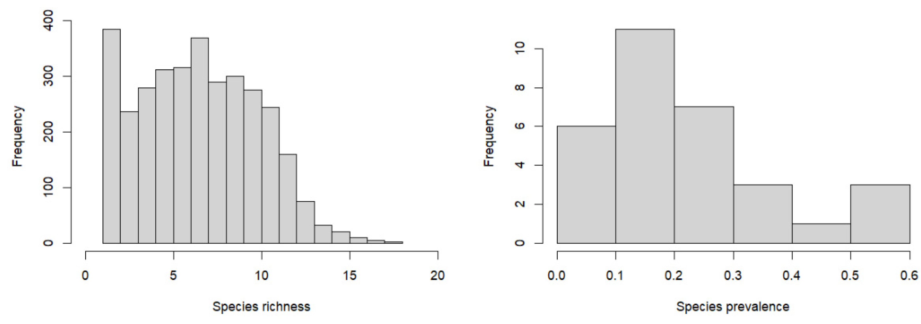
3.1. Tree Species Distribution Patterns

The richness (frequency of occurrence of tree species within permanent sample plots) and prevalence (proportion of plots in which a given tree species appears out of the total surveyed plots) distributions of these 31 tree species are shown in Figure 3. The richness of tree species varies significantly across plots, ranging from 1 to 18 (plots with ≤3 species account for 18.77%, and those with >10 species account for 16.50%). The prevalence of tree species ranges from 5% to 60%, reflecting that the tree species selected in this study include both common and rare species (top three prevalent common species—Acer mono 59.78%, Quercus mongolica 55.03%, Tilia amurensis 54.37%; top three prevalent rare species—Salix matsudana 3.35%, Populus tremula 3.93%, Pinus sibirica 4.08%).

3.2. Model Interpretability and Predictive Power

3.2.1. Overall Evaluation of Interpretability and Predictive Power of the Three Models

For the models FULL, ENV, and SPACE, their interpretability was evaluated by calculating two indicators, AUC and Tjur R². Cross-validation was conducted based on plot numbers using a two-fold sampling method, and both AUC and Tjur R² were calculated to evaluate the models’ predictive power (

Table 2. The evaluation of HMSC model.

Models	Fitting		Cross Validation
	AUC	Tjur R2	AUC	Tjur R2
Model FULL	0.8325	0.2326	0.6940	0.1412
Model ENV	0.7664	0.1454	0.7528	0.1399
Model SPACE	0.7297	0.1346	0.6719	0.0705

).

Table 2 indicates that, in terms of model fitting, the AUC and Tjur R² metrics show consistent results, reflecting that, in terms of interpretability, model FULL > model ENV > model SPACE. However, in the cross-validation, the performance of model SPACE was slightly worse than the other two models. The AUC metric shows that model ENV performed better than model FULL, but the Tjur R² metric shows that its performance was slightly worse than model FULL. By comparing the evaluation results of cross-validation and model fitting, it can be seen that spatial random effects significantly improve the model’s fitting effectiveness (AUC increased by 8.62%, Tjur R² increased by 60.04%), but its predictive effect is not ideal (AUC actually decreased by 7.81%, Tjur R² increased by 0.97%). The inclusion of spatial random effects in model FULL led to a significant drop in both AUC and Tjur R² metrics in cross-validation (AUC decreased by 16.64%, Tjur R² decreased by 39.30%). The cross-validation indicators for model ENV were close to those of the model fitting (AUC decreased by 1.78%, Tjur R² decreased by 3.79%), indicating that this model maintains consistency in both interpretability and predictive power. At first glance, the interpretability of model SPACE being greater than zero is questionable since it does not contain environmental covariates, but it does have a spatial random effects part, which contributes to its interpretability. However, the random effects part has limited help in predicting new plots (AUC decreased by 7.92%, Tjur R² decreased by 47.62%), as shown by the predictive power of model SPACE based on cross-validation (Tjur R² value is 0.0705), suggesting there is overlap in information between environmental covariates and spatial coordinates. In summary, whether considering interpretability or predictive power, and whether evaluated by AUC or Tjur R² for model fitting effectiveness, model FULL and ENV perform as expected without overfitting, while model SPACE might have overfitting issues.

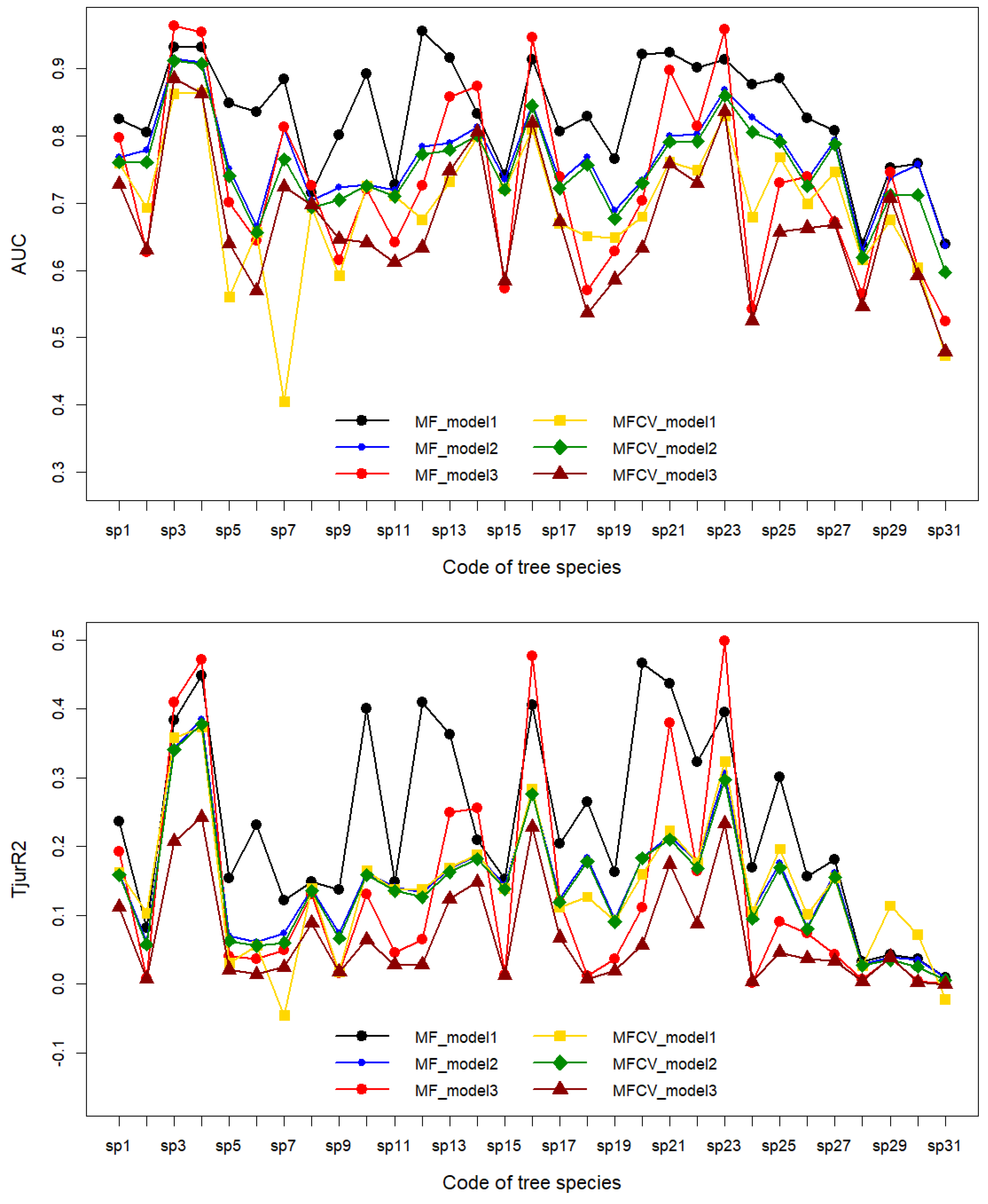
3.2.2. Evaluation of Interpretability and Predictive Power by Tree Species

Combining the model forms—model FULL (model 1), model ENV (model 2), and model SPACE (model 3)—with the type of model prediction, i.e., interpretability (MF) and predictive power (MFCV), six combination schemes are formed. The evaluation of these 31 tree species using AUC and Tjur R² metrics is displayed in Figure 4. The results reflected by the AUC and Tjur R² metrics for the distribution of the 31 tree species are consistent across all models, indicating that, within the same model, interpretability exceeds predictive power. This outcome is expected since interpretability uncovers all the information within the data. The interpretability and predictive power of the 31 tree species in model ENV are almost identical, resembling the predictive power of model FULL, suggesting that model ENV has stable extrapolation capabilities.

There are significant differences in the HMSC model fits among the 31 tree species in the study area, with AUC and Tjur R² metrics showing a consistent pattern of differences between interpretability and predictive power: model FULL > model SPACE > model ENV. For example, considering AUC values, the top three species with the largest difference in model FULL are as follows: Pinus sibirica (sp7, 0.48), Pinus sylvestris (sp5, 0.29), and Ulmus pumila (sp12, 0.28). The top three species with the largest difference in model SPACE are as follows: Acer ukurunduense (sp21, 0.14), Betula ermanii (sp16, 0.13), and Acer ginnala (sp23, 0.12). The top three species with the largest difference in model ENV are as follows: Populus tremula (sp30, 0.05), Pinus sibirica (sp7, 0.05), and Salix matsudana (sp31, 0.04). Furthermore, in terms of consistency and good fit between model interpretability and predictive power, the results for tree species in model FULL and ENV are consistent, including Picea jezoensis (sp3), Abies nephrolepis (sp4), and Acer ginnala (sp23). Notably, in model SPACE, Picea jezoensis (sp3), Abies nephrolepis (sp4), Betula ermanii (sp16), and Acer ginnala (sp23) all exhibit the best interpretability and predictive power, even exceeding model FULL. Among the more prevalent tree species, those with good interpretability and predictive power in model FULL include the following: Pinus koraiensis (sp1, MF: 0.83, MFCV: 0.76), Tilia amurensis (sp10, MF: 0.89, MFCV: 0.73), Ulmus laciniata (sp13, MF: 0.92, MFCV: 0.73), Betula ermanii (sp16, MF: 0.91, MFCV: 0.81), Acer ukurunduense (sp21, MF: 0.92, MFCV: 0.76), and Acer pseudosieboldianum (sp25, MF: 0.89, MFCV: 0.77).

3.3. Variance Contribution of Environmental Covariates

The study first investigates the variance contribution of environmental covariates to the models, i.e., variance partitioning for these three model types. Since model SPACE only contains spatial random effects, all explained variance is attributed to random effects. Therefore, comparisons between model FULL and ENV will more clearly demonstrate the importance of environmental covariates and spatial random effects in explaining community ecosystems.

The environmental covariates are grouped as follows: average temperature of the hottest quarter (Tave_JJA), rainfall of the hottest quarter (PPT_JJA), number of frost-free days per year (NFFD), annual humidex (AHM), evapotranspiration (Eref), average temperature of the coldest month (MCMT), and the temperature difference between the hottest and coldest months (TD) are grouped as climate variables; elevation (ELE) as a site variable; and bulk density of soil particles (bdod), soil organic carbon content (soc), proportion of coarse fragments (cfvo), and soil pH value (phh2o) as soil variables. For simplicity, the intercept is allocated to climate variables. The variance contribution rates of the model components are shown in

Table 3. The variance partition of models FULL, ENV, and SPACE.

Models	Climate	Site	Soil	Random
Model FULL	0.5742	0.1275	0.0914	0.2069
Model ENV	0.7322	0.1617	0.1061	0.0000
Model SPACE	0.0000	0.0000	0.0000	1.0000

. It is observed that the ranking of environmental factors explaining model variance is as follows: climate > site > soil. The two components of environmental change (climate and site) explain a significant portion of the model variance, with soil factors being the weakest. The variance contribution of spatial random effects is also significant, with the importance of specific environmental factors varying by tree species.

The variance contribution results of model ENV also indicate that the ranking of environmental factors explaining model variance is as follows: climate > site > soil, consistent with what is shown by model FULL. Two species are dominated by site factors, each with a variance contribution rate of over 45%, specifically Ulmus japonica (sp11, 0.62) and Tilia amurensis (sp9, 0.47), with the remaining 29 species being dominated by climate factors. The results of the variance partitioning indicate that model FULL has a substantial dependency on spatial random effects for some species, which also explains the performance differences between it and model ENV. Moreover, climate change explains nearly five times the model variability than site changes.

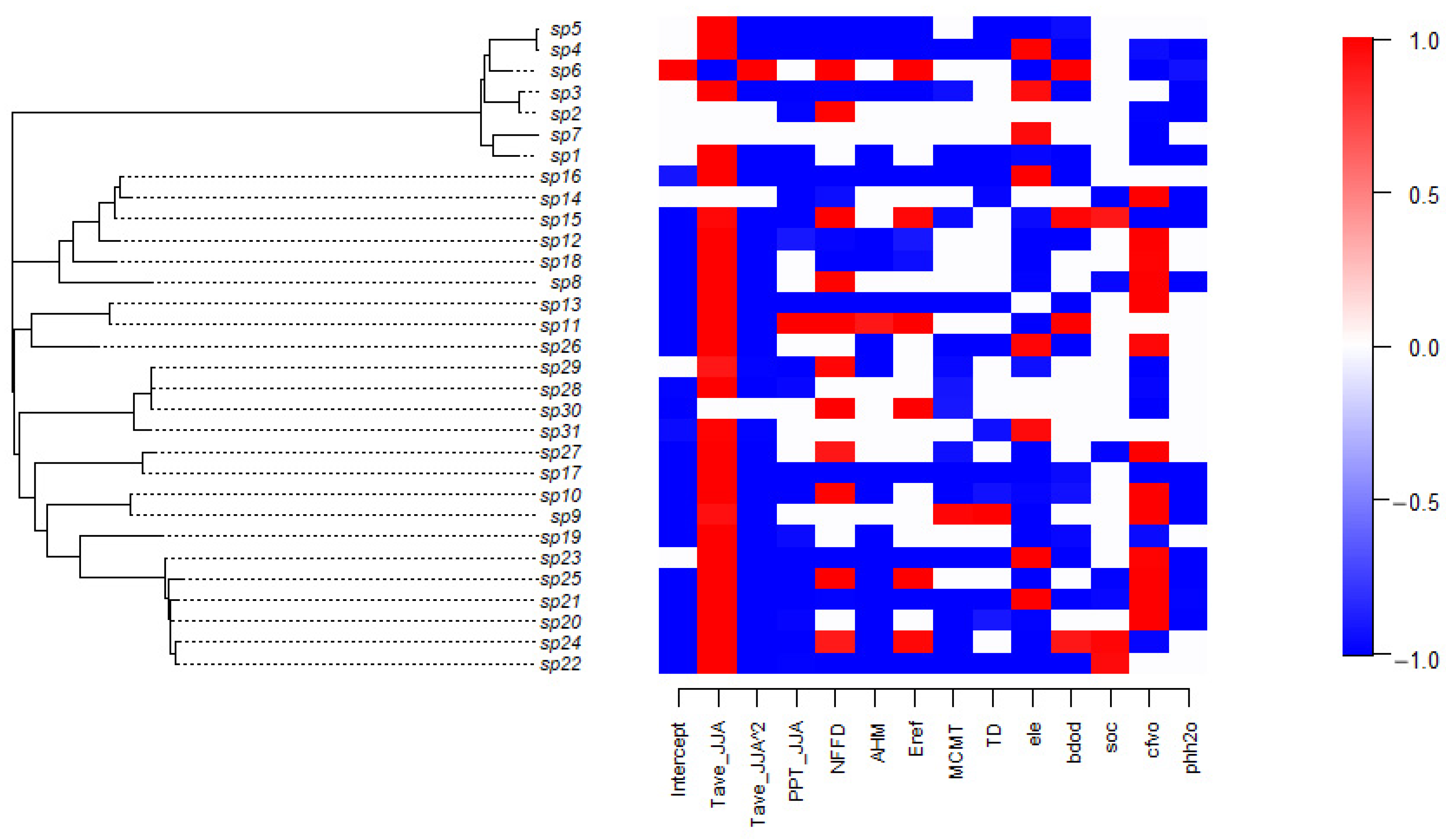
3.4. Tree Species Niches

To examine the differences between the niches of tree species, this study utilized a visualization method to display the response relationships of the 31 tree species to environmental covariates in model FULL, representing the niches of tree species (Figure 5). Figure 5 provides strong statistical support for the posterior distribution, showing either positive (red) or negative (blue) relationships, indicating clear environmental filtering signals. For most tree species, there is a significant parabolic relationship between their presence and the average temperature of the hottest quarter. Due to the negative coefficient of the quadratic term, there is an optimal temperature for their existence. Their responses to environmental factors (rainfall in the hottest quarter PPT_JJA, annual humidex AHM, average temperature of the coldest month MCMT, the temperature difference between the hottest and coldest months TD, and soil pH value phh2o) are negative, while their preferences for the number of frost-free days per year NFFD, evapotranspiration Eref, elevation ele, bulk density of soil particles bdod, soil organic carbon content soc, and the proportion of coarse fragments cfvo vary. In terms of the relationship between various tree species and environmental covariates, Larix olgensis (sp6), Ulmus japonica (sp11), Betula platyphylla (sp15), and Acer triflorum (sp24) show a more positive response.

The visualization results of tree species niches in model ENV are similar to those in model FULL, with the difference being that the response of some tree species to environmental covariates shifts from positive to non-correlated. For instance, in model ENV, the response relationship to the number of frost-free days per year (NFFD) for Tilia amurensis (sp10), Acer triflorum (sp24), and Fraxinus rhynchophylla (sp27) show non-correlation. Ulmus japonica (sp11)’s response to the annual humidex AHM and Acer triflorum (sp24)’s response to evapotranspiration Eref are non-correlated.

4. Discussion

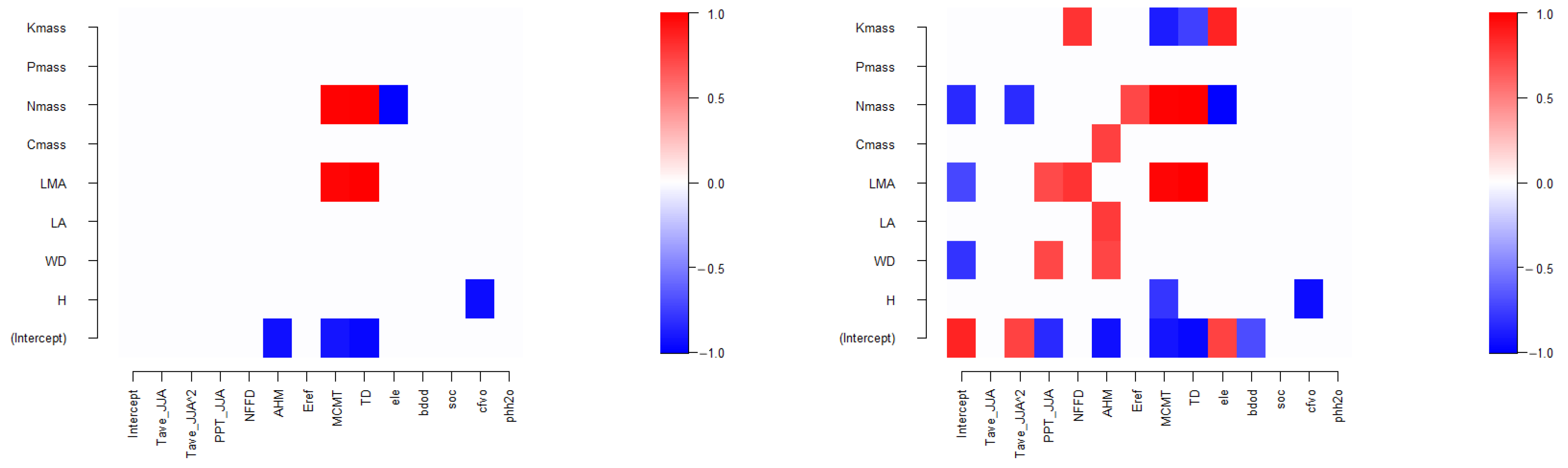
4.1. Relationship between Tree Species Niches and Traits—Phylogeny

The HMSC models tree species niches (parameters β) as a function of tree species traits (regression parameters γ) and phylogeny (phylogenetic signal parameters ρ); thus, these connections can be explored by plotting parameter estimates for tree species communities [16]. First, we investigate whether there is a correlated relationship between tree species niches and their traits and phylogeny in model FULL (Figure 6). At a posterior distribution statistical support level of 0.95, it indicates that the response of tree species to environmental covariates (average temperature of the coldest month MCMT and the temperature difference between the hottest and coldest months TD) is positively correlated with tree species traits (leaf dry matter density, LMA, and leaf nitrogen concentration, Nmass), while elevation, ele, is negatively correlated with leaf nitrogen concentration, Nmass, and the proportion of coarse fragments, cfvo, is negatively correlated with maximum tree height, H (Figure 6 left). When reducing the statistical support level to 0.85, a richer relationship between tree species niches and traits is observed (Figure 6 right). The relationships revealed by model ENV are mostly consistent, for example, at the 0.95 level, elevation, ele, is not correlated with leaf nitrogen concentration, Nmass.

Another method of examining the impact of tree species traits is to evaluate how much variation they explain in the response of tree species to their environmental covariates (

Table 4. The explanatory power of species traits.

Models		Model FULL	Model ENV
Environmental covariates	Intercept	0.3291	0.2521
	Tave_JJA	0.0881	0.0659
	Tave_JJA2	0.1521	0.0935
	PPT_JJA	0.1458	0.1254
	NFFD	0.0684	0.0839
	AHM	0.0541	0.0471
	Eref	0.0405	0.0494
	MCMT	0.4355	0.4569
	TD	0.4393	0.4522
	ele	0.3504	0.3229
	bdod	0.0418	0.0444
	soc	0.0394	0.0406
	cfvo	0.2119	0.1812
	phh2o	0.0677	0.0515
Species occurrence		0.1832	0.1797

). Leaf dry matter density, LMA, leaf nitrogen concentration, Nmass, and maximum tree height, H, explain a significant portion of the environmental covariate variation, while the remaining tree species traits only explain a small part of the environmental covariate variation; this is consistent with the patterns presented in Figure 5. Further quantification of the variance in the occurrence dependent variable of tree species explained by tree species traits reveals the same pattern, i.e., the contribution to explained variance is not high (0.1832 for model FULL and 0.1797 for model ENV). Comparing models FULL and ENV, the former shows a slight improvement in the degree to which tree species traits explain the variance of environmental covariates and the occurrence dependent variable, which may be due in part to the contribution of spatial random effects in model FULL.

Further, examining the strength of the phylogenetic signal in tree species niches, the percentiles of the parameter for the phylogenetic signal are statistically obtained from the posterior distribution. (Model FULL: 2.5%, 0.24; 50%, 0.48; 97.5%, 0.67. Model ENV, 2.5%, 0.31; 50%, 0.55; 97.5%, 0.71.) This clearly indicates the presence of a phylogenetic signal within the tree species niches. This suggests that the trait factors affecting tree species niches that are missing in the data have a phylogenetic structure [16,34]. Additionally, the average value of the parameter representing the strength of the phylogenetic signal in model FULL is 0.47, slightly lower than 0.54 in model ENV, indicating that spatial random effects reduce the impact of missing tree species trait factors on tree species niches to some extent [16].

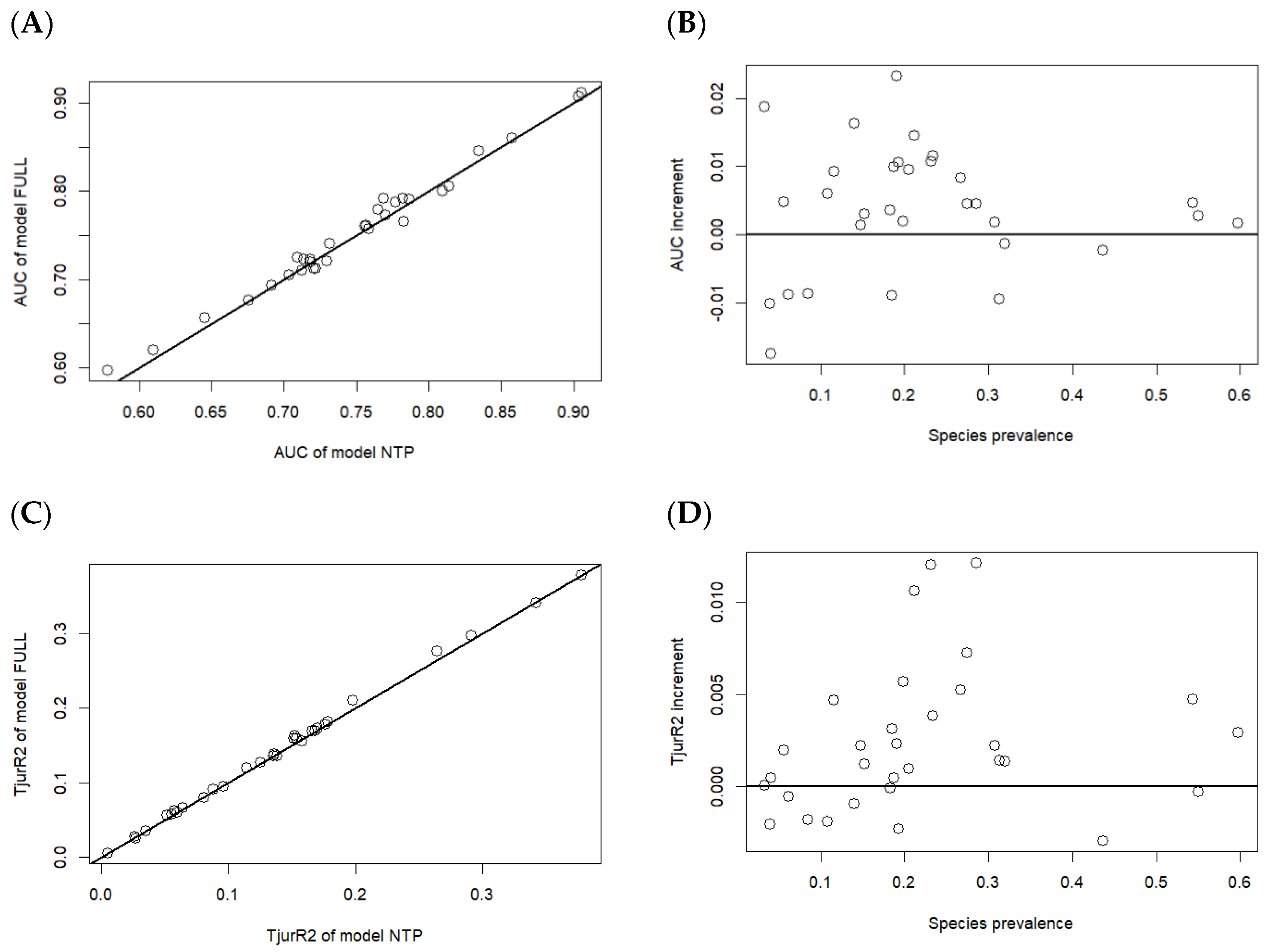
4.2. Impact of Introducing Tree Species Traits and Phylogenetic Trees on Prediction

The HMSC model uses tree species trait data to estimate parameters reflecting the response of tree species traits on their niches and uses tree species phylogenetic information to estimate parameters indicating the strength of the phylogenetic signal in tree species niches. These two parameters integrate tree-level information into community-level parameters, hence incorporating tree species traits and phylogeny into the model helps to synthesize information extracted from community data. However, whether the introduction of tree species traits and phylogeny can enhance the predictive ability of the HMSC model still needs to be assessed [16]. To this end, a new model, NTP, which does not include information on tree species traits and phylogeny, was set up on the basis of model FULL and applied to the same data. The predictive evaluation metrics AUC and Tjur R² of both models were then compared in cross-validation (Figure 7).

The comparison between model FULL and NTP (Figure 7) shows that the patterns reflected by the indicators AUC and Tjur R² are consistent. The predictive ability gap between model FULL and NTP is very small, and this difference diminishes as the prevalence of tree species increases. On average, the model including tree species traits and phylogeny performs better, especially for rare tree species that are typically difficult to predict accurately. This is because the introduction of traits and phylogeny allows the model to borrow information from other tree species, especially those with similar traits and closely related phylogenies. For tree species that occur infrequently in the data, this minor information can make a significant difference [34]. In contrast, tree species with sufficient data do not need to borrow information from others, which explains why the difference between the two models decreases when the species prevalence approaches 0.3.

As mentioned above, the introduction of tree species traits and phylogeny in the HMSC model can enhance the predictive ability for evaluating tree species occurrence. However, the contribution of tree species traits to explain the variation of tree species occurrence is not high, and there are phylogenetic signals in tree species niches, which means that the relevant tree species traits affecting tree species niches are missing in the data. Therefore, it is necessary to find suitable tree species traits for improving the prediction of tree species occurrence, especially for rare tree species in further study [34]. Additionally, we can use tree species traits and phylogeny in the HMSC model to study the biotic relationship between tree species in following research [22,35].

5. Conclusions

This study employed the widely used hierarchical modeling of species communities (HMSC) to fit the distribution data of multiple tree species in Jilin Province. The data types included the presence or abundance of tree species from the ninth National Forest Inventory in 2014, environmental factors corresponding to the plots (site, soil, or climate data), tree species functional traits (maximum tree height, wood density, and leaf area index, etc.), phylogenetic relationships of tree species, and the geographic coordinates of the plots. A joint species distribution model for multiple tree species was constructed, including model structure design, selection of predictive factors, MCMC convergence test of model parameters, and model evaluation and comparison. The HMSC fitting determined environmental factors or tree species trait factors, establishing the joint species distribution model with the best fitting effect. Finally, the application and extension of the constructed joint species distribution model included interpreting tree species niches, studying the relationship between tree species niches and tree species traits and phylogeny, and the results of model comparison indicating that the information conveyed by environmental and spatial predictors overlaps to some extent. Therefore, the choice between model FULL and ENV should be based on the purpose of the model’s use, not the difference in predictive ability.

References

1. Duan, G.; Lei, X.; Zhang, X.; Liu, X. Site index modeling of larch using a mixed-effects model across regional site types in northern China. Forests 2022, 13, 815. [Google Scholar] [CrossRef]
2. Hu, X.F.; Duan, G.S.; Zhang, H.R. Modelling individual tree diameter growth of Quercus mongolica secondary forest in the northeast of China. Sustainability 2021, 13, 4533. [Google Scholar] [CrossRef]
3. National Forestry and Grassland Administration. China Forest Resources Report 2014–2018; China Forestry Publishing House: Beijing, China, 2019. (In Chinese)
4. Liu, D. Research on Quantitative Place Suitability and Tree Suitability Based on Distribution Suitability and Potential Productivity; Chinese Academy of Forestry: Beijing, China, 2018. (In Chinese) [Google Scholar]
5. Lan, J.; Lei, X.; He, X.; Gao, W.; Guo, H. Stand density, climate and biodiversity jointly regulate the multifunctionality of natural forest ecosystems in northeast China. Eur. J. For. Res. 2023, 142, 493–507. [Google Scholar] [CrossRef]
6. Leng, W.; He, H.S.; Bu, R.; Dai, L.; Hu, Y.; Wang, X. Predicting the distributions of suitable habitat for three larch species under climate warming in northeastern China. For. Ecol. Manag. 2008, 254, 420–428. [Google Scholar] [CrossRef]
7. Wang, X.; Fang, J.; Sanders, N.J.; White, P.S.; Tang, Z. Relative importance of climate vs local factors in shaping the regional patterns of forest plant richness across northeast China. Ecography 2009, 32, 133–142. [Google Scholar] [CrossRef]
8. Yin, X.J.; Zhou, G.S.; Sui, X.H.; He, Q.J.; Li, R.P. Dominant climatic factors and their thresholds in the geographical distribution of Quercus mongolica. Acta Ecol. Sin. 2013, 33, 103–109. (In Chinese) [Google Scholar]
9. Liu, D.; Li, Y.T.; Hong, L.X.; Guo, H.; Xie, Y.S.; Zhang, Z.L.; Lei, X.D.; Tang, S.Z. Potential distribution suitability of major natural forests in Jilin Province based on maximum entropy model. Sci. Silvernica Sin. 2018, 54, 1–15. (In Chinese) [Google Scholar]
10. Pugnaire, F.I. Positive Plant Interactions and Community Dynamics; CRC Press: Boca Raton, FL, USA, 2010. [Google Scholar]
11. Wisz, M.S.; Pottier, J.; Kissling, W.D.; Pellissier, L.; Lenoir, J.; Damgaard, C.F.; Dormann, C.F.; Forchhammer, M.C.; Grytnes, J.-A.; Guisan, A.; et al. The role of biotic interactions in shaping distributions and realised assemblages of species: Implications for species distribution modelling. Biol. Rev. 2013, 88, 15–30. [Google Scholar] [CrossRef]
12. Barrero, A.; Ovaskainen, O.; Traba, J.; Gómez-Catasús, J. Co-occurrence patterns in a steppe bird community: Insights into the role of dominance and competition. Oikos 2023, 2023, e09780. [Google Scholar] [CrossRef]
13. Ovaskainen, O.; Soininen, J. Making more out of sparse data: Hierarchical modeling of species communities. Ecology 2011, 92, 289–295. [Google Scholar] [CrossRef]
14. Randin, C.F.; Ashcroft, M.B.; Bolliger, J.; Cavender-Bares, J.; Coops, N.C.; Dullinger, S.; Dirnböck, T.; Eckert, S.; Ellis, E.; Fernández, N.; et al. Monitoring biodiversity in the Anthropocene using remote sensing in species distribution models. Remote Sens. Environ. 2020, 239, 111626. [Google Scholar] [CrossRef]
15. Chardon, N.I.; Pironon, S.; Peterson, M.L.; Doak, D.F. Incorporating intraspecific variation into species distribution models improves distribution predictions, but cannot predict species traits for a wide-spread plant species. Ecography 2020, 43, 60–74. [Google Scholar] [CrossRef]
16. Ovaskainen, O.; Abrego, N. Joint Species Distribution Modelling with Applications in R; Cambridge University Press: Cambridge, UK, 2020. [Google Scholar]
17. Clark, J.S.; Gelfand, A.E.; Woodall, C.W.; Zhu, K. More than the sum of the parts: Forest climate response from joint species distribution models. Ecol. Appl. 2014, 24, 990–999. [Google Scholar] [CrossRef] [PubMed]
18. Warton, D.I.; Blanchet, F.G.; O’hara, R.B.; Ovaskainen, O.; Taskinen, S.; Walker, S.C.; Hui, F.K. So many variables: Joint modeling in community ecology. Trends Ecol. Evol. 2015, 30, 766–779. [Google Scholar] [CrossRef] [PubMed]
19. Harris, D.J. Generating realistic assemblages with a joint species distribution model. Methods Ecol. Evol. 2015, 6, 465–473. [Google Scholar] [CrossRef]
20. Hui, F.K.C. Boral-Bayesian ordination and regression analysis of multivariate abundance data in r. Methods Ecol. Evol. 2016, 7, 744–750. [Google Scholar] [CrossRef]
21. Ovaskainen, O.; Tikhonov, G.; Norberg, A.; Blanchet, F.G.; Duan, L.; Dunson, D.; Roslin, T.; Abrego, N. How to make more out of community data? A conceptual framework and its implementation as models and software. Ecol. Lett. 2017, 20, 561–576. [Google Scholar] [CrossRef] [PubMed]
22. Zurell, D.; Pollock, L.J.; Thuiller, W. Do joint species distribution models reliably detect interspecific interactions from co-occurrence data in homogenous environments. Ecography 2018, 41, 1812–1819. [Google Scholar] [CrossRef]
23. Wang, T.; Wang, G.; Innes, J.L.; Seely, B.; Chen, B. ClimateAP: An application for dynamic local downscaling of historical and future climate data in Asia Pacific. Front. Agric. Sci. Eng. 2017, 4, 448–458. [Google Scholar] [CrossRef]
24. Poggio, L.; de Sousa, L.M.; Batjes, N.H.; Heuvelink, G.B.M.; Kempen, B.; Ribeiro, E.; Rossiter, D. SoilGrids 2.0: Producing soil information for the globe with quantified spatial uncertainty. Soil 2021, 7, 217–240. [Google Scholar] [CrossRef]
25. Tikhonov, G.; Duan, L.; Abrego, N.; Newell, G.; White, M.; Dunson, D.; Ovaskainen, O. Computationally efficient joint species distribution modeling of big spatial data. Ecology 2019, 101, e02929. [Google Scholar] [CrossRef] [PubMed]
26. Norberg, A.; Abrego, N.; Blanchet, F.G.; Adler, F.R.; Anderson, B.J.; Anttila, J.; Araújo, M.B.; Dallas, T.; Dunson, D.; Elith, J.; et al. A comprehensive evaluation of predictive performance of 33 species distribution models at species and community levels. Ecol. Monogr. 2019, 89, e01370. [Google Scholar] [CrossRef]
27. Tjur, T. Coefficients of determination in logistic regression models a new proposal: The coefficient of discrimination. Am. Stat. 2009, 63, 366–372. [Google Scholar] [CrossRef]
28. Valavi, R.; Guillera-Arroita, G.; Lahoz-Monfort, J.J.; Elith, J. Predictive performance of presence-only species distribution models: A benchmark study with reproducible code. Ecol. Monogr. 2022, 92, e01486. [Google Scholar] [CrossRef]
29. Tikhonov, G.; Opedal, H.; Abrego, N.; Lehikoinen, A.; de Jonge, M.M.J.; Oksanen, J.; Ovaskainen, O. Joint species distribution modelling with the R-package Hmsc. Methods Ecol. Evol. 2020, 11, 442–447. [Google Scholar] [CrossRef] [PubMed]
30. Abrego, N.; Ovaskainen, O. Evaluating the predictive performance of presence–absence models: Why can the same model appear excellent or poor? Ecol. Evol. 2023, 13, e10784. [Google Scholar] [CrossRef] [PubMed]
31. Wickham, H.; François, R.; Henry, L.; Müller, K. dplyr: A Grammar of Data Manipulation. R Package Version 1.1.2. 2023. Available online: https://CRAN.R-project.org/package=dplyr (accessed on 15 October 2023).
32. Wickham, H. ggplot2: Elegant Graphics for Data Analysis; Springer: New York, NY, USA, 2016. [Google Scholar]
33. Tikhonov, G.; Ovaskainen, O.; Oksanen, J.; De Jonge, M.; Opedal, O.; Dallas, T. Hmsc: Hierarchical Model of Species Communities. R Package Version 3.0-13. 2022. Available online: https://CRAN.R-project.org/package=Hmsc (accessed on 15 October 2023).
34. Zhang, C.; Chen, Y.; Xu, B.; Xue, Y.; Ren, Y. Improving prediction of rare species’ distribution from community data. Sci. Rep. 2020, 10, 12230. [Google Scholar] [CrossRef]
35. Blanco-Cano, L.; Navarro-Cerrillo, R.M.; González-Moreno, P. Biotic and abiotic effects determining the resilience of conifer mountain forests: The case study of the endangered Spanish fir. For. Ecol. Manag. 2022, 520, 120356. [Google Scholar] [CrossRef]
Figure 1. The distribution map of permanent sample plots used in the study in Jilin province.
Forests 15 01026 g001
Figure 2. The phylogenetic tree of 31 tree species in this study.
Forests 15 01026 g002
Figure 3. Tree species distribution frequency of the community data (for species richness (left), the y-axis (frequency) corresponds to the number of sampling plots, and the x-axis to the number of species in each sampling plot; for species prevalence (right), the y-axis (frequency) corresponds to the number of species, and the x-axis to the fraction of sampling plots in which the species is present).
Forests 15 01026 g003
Figure 4. The evaluation of 31 tree species for HMSC model.
Forests 15 01026 g004
Figure 5. Heatmap of estimated parameters β of model FULL, i.e., species niches. Red and blue colors show parameters that are estimated to be positive and negative, respectively (with at least 0.95 posterior probability in Model FULL).
Forests 15 01026 g005
Figure 6. Heatmap of estimated parameters γ linking species traits to species niches of model FULL. Red and blue colors show parameters that are estimated to be positive and negative, respectively (with at least 0.95 posterior probability in the left, and 0.85 in the right).
Forests 15 01026 g006
Figure 7. Difference in predictive power between models that include traits and phylogeny versus those that do not. In four panels, each dot corresponds to one tree species. Panel (A) shows the AUC statistic for the models that do (y-axis) and do not (x-axis) include traits and phylogeny. Panel (B) shows the difference in AUC between the two models as a function of species prevalence. Positive values of AUC increment indicate that the model with traits and phylogeny performs better in cross-validation. The same as panels (C,D) for index Tjur R2, respectively.
Forests 15 01026 g007