Article

Characteristics and Driving Mechanisms of Understory Vegetation Diversity Patterns in Central and Southern China

1
Hunan Academy of Forestry, No. 658 Shaoshan Road, Changsha 410004, China
2
Hunan Cili Forest Ecosystem National Observation and Research Station, Cili 427200, China
*
Author to whom correspondence should be addressed.
Forests 2024, 15(6), 1056; https://doi.org/10.3390/f15061056
Submission received: 15 April 2024 / Revised: 11 June 2024 / Accepted: 14 June 2024 / Published: 18 June 2024
(This article belongs to the Section Forest Biodiversity)

Abstract

:
Large-scale forest restoration projects significantly reduce the net rates of forest loss. However, as a key component of forest restoration, planted forests have failed to restore biodiversity. China has implemented a large-scale afforestation program, which includes pure planted forests in particular, leading to various changes in ecosystem processes. Despite this, a comprehensive analysis of understory vegetation diversity patterns in these pure planted forests is still lacking. This study aimed to analyze the data on understory vegetation diversity from three typical pure and natural forest ecosystems of Hunan ecological forests to reveal their diversity patterns. The results revealed no significant difference in the understory diversity index between natural and pure forest types, although natural forests had a bigger species pool. The Zipf–Mandelbrot model was a better fit for species abundance distribution. The fitted results suggested that both environmental filtering and neutral processes affected the species abundance distribution and pure understory communities during restoration succession. Natural forests had the most stable understory diversity structure, whereas pure Phyllostachys heterocycla (Carr.) Mitford forests had the least stable structure. Multivariate regression tree analysis identified indicator species for each community. The gradient boosting model indicated that isothermality and slope direction were the most important factors affecting diversity. The β-diversity analysis showed that community establishment in the four forest types was affected via different mechanisms. The findings of this study have significant implications for understanding the impact of afforestation on the mechanisms for maintaining diversity.

1. Introduction

Biodiversity has always been the core issue of macro-ecology research. Understanding the patterns and mechanisms of diversity is crucial for developing sustainable and effective conservation strategies, but it also presents numerous challenges for ecologists [1,2]. Species richness is often used to identify species abundance distribution (SAD) [3]. SAD describes the proportional abundance of species within a community [4]. It has also been considered one of the most fundamental descriptors of a particular community. The SAD models can be categorized into empirical statistical models, niche models, and community-neutral theory models [5]. Comparing different SAD models is often useful for detecting disturbances in ecosystems, explaining resource allocation, and understanding interspecific associations [3,6,7].
Community assembly is a central topic in community ecology, with ecologists striving to explain its driving mechanisms. Hence, most theories can be broadly summarized into two conceptual frameworks: neutral and niche theories. The niche theory emphasizes the importance of deterministic processes, such as environmental factors [8,9]. In contrast, the neutral theory suggests that community assembly is a stochastic process, with dispersal limitations playing a dominant role [10]. β-diversity describes the variability among communities on temporal and spatial scales, which is crucial for understanding community assembly processes [11]. The effects of environmental factors and spatial distance on β-diversity are commonly used to assess ecological niches and neutral processes. The relationship between environmental variables, latitudes, and β-diversity reveals the assembly mechanisms of communities in the forests of northeastern China [12]. Tan et al. [13] found that dispersal limitation increased β-diversity in the Changbai Mountains. Turnover and nestedness are two different methods of illustrating the variation in species composition [14]. Turnover refers to replacing species along an ecological gradient, implying simultaneous species gain and losses due to environmental filtering, species competition, and historical events [15]. Nestedness occurs when one community includes a larger number of species than another, typically due to specific environmental processes [14]. Comparing turnover and nestedness has significant implications for biodiversity conservation [16].
Timber production has been the primary objective of forest management in recent decades. However, multiple ecosystem services (such as biodiversity as a whole) of forests have gained increasing attention. As a widely used strategy in forest management, afforestation can reduce atmospheric CO2 concentrations by increasing plant biomass and serving as a carbon sink [17,18]. China has implemented large-scale afforestation programs, leading to several ecological issues, such as reduced biodiversity, water loss, and changes in nutrient exchange processes [19]. Forests provide habitats for much of the world’s biodiversity, making biodiversity protection a critical task in forest management [20]. Previous studies have shown that an increase in forest area does not necessarily lead to the restoration of forest structure and function, which are often determined by biodiversity [21,22]. The current monitoring of planted forests remains coarse, primarily focusing on stand area and tree volume. A biodiversity-oriented target is needed, emphasizing the types and quantities of vegetation (trees, shrubs, and herbs), to more accurately assess the effectiveness of forest restoration [23]. Understory vegetation is a key component of forest ecosystems. It plays a crucial role in maintaining ecological functional stability [24] and revealing dynamic adaptive features to the environment [25,26]. Factors such as forest type [27], stand stage [19], and forest thinning [28] can significantly affect understory diversity.
The subtropical broad-leaved evergreen forest areas of Hunan Province, in central and south China, are considered the center of biodiversity in China. This region features a complex terrain dominated by mountains and hills, with an uneven distribution of hydrothermal resources. Among the planted pure forest types in the study area, forests dominated by pure forms Cunninghamia lanceolata (Lamb.) Hook., Pinus massoniana Lamb., and Phyllostachys heterocycla (Carr.) Mitford are the most widely distributed and typical. An in-depth understanding of the understory diversity patterns in these forests may help enhance forest management.
This study aimed to answer the following questions: (1) Did the patterns of understory vegetation diversity differ between pure forests and natural broadleaf forests? (2) What was the mechanism of community assembly? (3) What were the governing factors affecting the community assembly?

2. Materials and Methods

2.1. Data Sources

The study targeted an ecological forest, which is a forest that maintains ecosystem services functions and is situated in Hunan Province, China. It is the most significant forest resource in Hunan Province, covering 36.65% of the total forest area and is highly protected. The diversity data were extracted from 683 fixed sample plots distributed across Hunan ecological forests (updated in 2019). The plot size was 1000 m2 (with the edge parallel to the contour line). Five small shrub plots (2 × 2 m2) were also established within each plot for detailed investigations. The stand dynamics, including tree species composition, altitude, slope position, soil type, and canopy density, were also investigated. Based on these attributes, the plots were categorized according to tree species, origin, composition, and so forth. The present study focused on the understory vegetation diversity of the three pure forest types and natural broad-leaved forests, as mentioned earlier. Therefore, the plots of four forest types were extracted from the database (Figure 1): pure C. lanceolata (PCL, 56 plots), P. massoniana (PPM, 41 plots), P. heterocycla (PPH, 48 plots), and natural broad-leaved forests (NBL, 44 plots). The shrub species data and stand dynamics were extracted. In addition, 19 biologically meaningful variables (bioclimatic variables) for each plot were extracted from WorldClim (http://www.worldclim.org/, accessed on 3 April 2020, Table 1).

2.2. Detection and Comparison of Vegetation Diversity Patterns

The α-diversity index provides a visual snapshot of a community’s species count and their relative abundance. Therefore, three α-diversity indices (richness, Shannon, and Pielou’s evenness) were selected for intuitive comparison between four forest types (NBL, PCL, PPH, and PPM), between pure (PCL + PPH + PPM) and NBL forests. Then, regression analysis was performed between Pielou’s evenness and latitude/altitude to detect any vertical/horizontal distribution patterns. A regional species pool comprises all species available to inhabit a focal site, which is a crucial indicator reflecting the diversity structure and assembly mechanisms. The species pool consists of two complementary components, observed diversity and dark diversity (unobserved species), with the latter often being overlooked [29,30]. We used three models (jackknife, Chao, and bootstrap models) to predict the species pool in each community so as to compare the diversity potential between pure and natural broadleaf forests [31,32].
SAD models display logarithmic species abundance against species rank order, offering a means to elucidate abundance distribution types and compare multiple diversity patterns. We first used five widely used SAD models (broken stick, niche preemption, log-normal, Zipf, and Zipf–Mandelbrot) to fit the data so as to further compare the diversity patterns of pure and natural broadleaf forests [28,33,34,35,36]. Then, we selected the best-fitting model based on Bayesian Information Criterion (BIC) indices, where smaller values indicated a better fit. Parameters γ and β, derived from the chosen model, were used to characterize the diversity structure. A lower γ value indicated a highly organized community with complex species interactions. Higher values of β indicated a high degree of niche diversification [37]. The aforementioned analyses were conducted using the R package “vegan.”

2.3. Exploring Mechanisms of Community Assembly

Mantel and partial-Mantel analyses were performed to assess the correlation of environmental/geographic distance with variations in diversity, thereby testing the two main hypotheses driving community assembly. The geographic distance was calculated using the R package “geosphere” based on coordinates. The environmental matrix and geographic distance were standardized. The environmental/geographic distance was visualized through scatter plots with linear regression using the R package “ggplot2” [38]. Additionally, the matrices of β-diversity were divided into decomposed, replacement, and richness differences using Jaccard indices, representing the triple values of similarity, richness difference, and replacement [14]. These calculations were performed using the R package “adespatial” [39].

2.4. Driving Factors of Community Assembly

The gradient boosting model (GBM) was used to assess the relative impact of the aforementioned driving factors (soil type, altitude, landform, density, tree coverage, slope direction, and 19 bioclimatic variables) on the Shannon index, using the R package “gambin” [40]. This model could be used to continuously fit the nonlinear relationship between diversity and factors. Its explanatory variable-selection cross-validation approach, along with its flexibility, provides significant advantages in ecological studies [41]. The marginal analysis was conducted to elucidate the interplay between two or three predictor variables.

3. Results

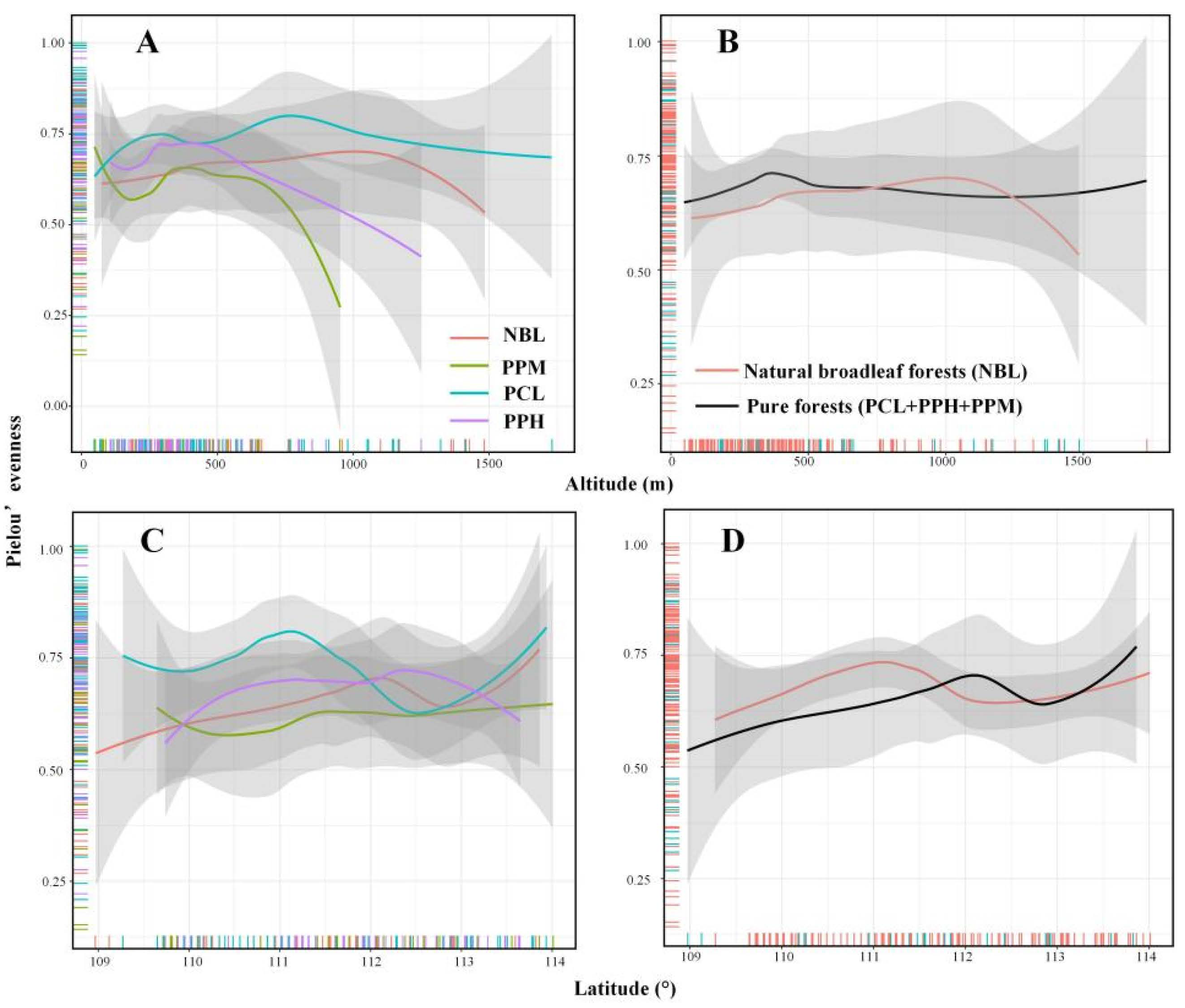
3.1. Vertical/Horizontal Diversity Distribution Pattern and Species Pool

The richness, Pielou’s evenness, and Shannon indices were calculated for the four populations, revealing no significant differences among them (Figure 2A–C, P = 0.05). Similarly, no significant differences were found in these indices between the pure (PCL + PPH + PPM) and natural broadleaf (NBL) forest populations (Figure 2D–F, P = 0.05). The regression analysis between the Pielou’s evenness index and latitude/altitude is shown in Figure 3. The diversity index of PCL, PPH, and NBL increased first and then decreased with the increase in altitude, exhibiting a single-peaked curve. Conversely, the diversity index of PPM initially decreased and then peaked below 500 m. The index of four communities exhibited a wavelike curve with the increase in latitude. The diversity index of pure forests showed different horizontal and vertical distribution patterns compared with NBL. Specifically, the peak value of pure forests occurred earlier than that of NBL with the increasing altitude (Figure 3B). The fitting curves between latitude and Pielou’s evenness for pure and natural broadleaf forests were similar, with the peak value of NBL occurring earlier than that of pure forests with increasing latitude (Figure 3D).
The species pools of the study area were estimated using three predicted models. The results (Table 2) indicated that the species pool predicted using the Chao model was the largest, followed by the jackknife and bootstrap models. For NBL, the predicted values were 528 (Chao), 346 (jackknife), and 263 (bootstrap). For PPM, PPH, and PCL, the predicted richness values were 456 (Chao), 266 (jackknife), and 204 (bootstrap); 375 (Chao), 312 (jackknife), and 245 (bootstrap); and 452 (Chao), 314 (jackknife), and 242 (bootstrap); respectively. Overall, the species pool of NBL was larger than those of pure forests.

3.2. Comparison of Multiple Diversity Patterns Based on SAD

The fitting results of the broken stick, log-normal, Zipf–Mandelbrot, and niche preemption models are shown in Table 3 and Figure 4. In the PCL forest, the species with the highest abundance exceeded 50 in numbers in PCL (Figure 3A), whereas in the other forest types, it was <30 in numbers (Figure 4B–D). The SAD curves for the Zipf and Zipf–Mandelbrot models overlapped in the PCL and NBL populations, indicating a similar fitting effect. The BIC values suggested that the Zipf–Mandelbrot and Zipf models were the optimal models for all communities. The Zipf–Mandelbrot model was the best fit for the PCL, PPM, and PPH populations, whereas the Zipf model best fit the NBL population. Therefore, the Zipf–Mandelbrot model was selected as the explanatory model. Hence, the γ values ranged from −0.86 (PPH) to −0.61 (NBL), indicating that the species organizational structure in the NBL population was the most balanced, followed by PPM (−0.71) and PCL (−0.80). PPH had the most unstable organizational structure. However, parameter β ranged from 2.08 × 10⁻⁵ (PCL) to 2.35 (PPH), suggesting that the dominance of the dominant species of PCL was much higher than that of the other three forest types.

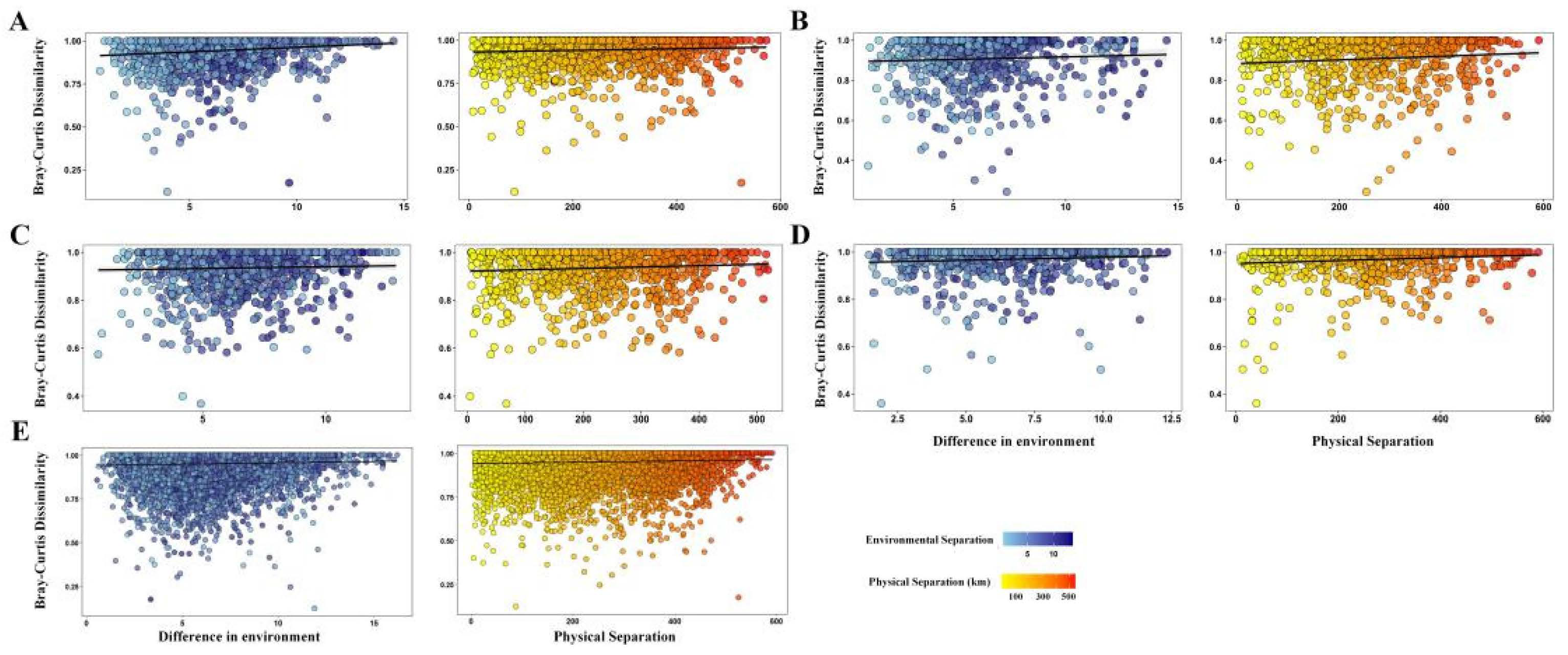
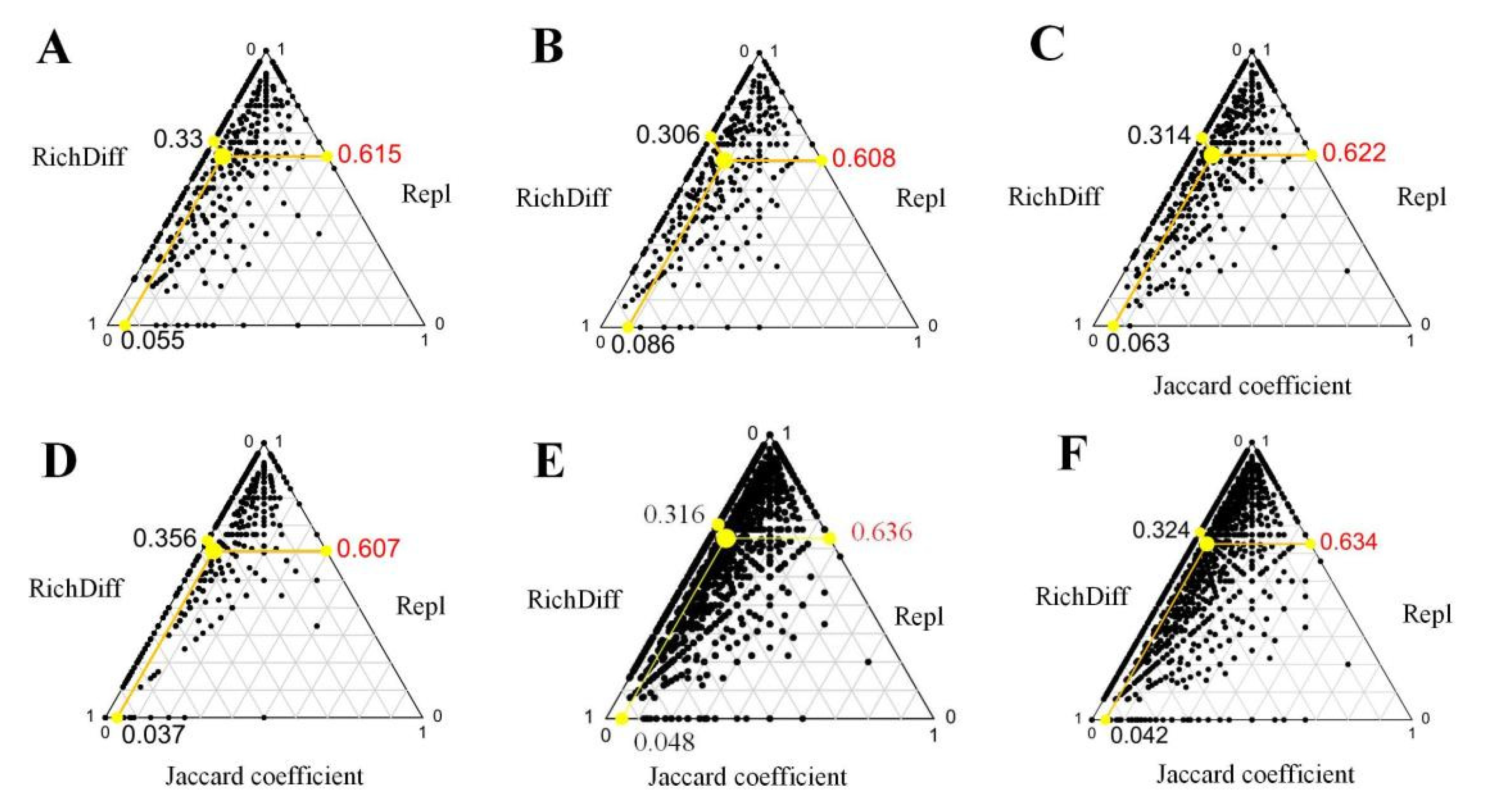
3.3. Mechanisms of Community Assembly

The linear regression showed an increasing trend between species composition and the environmental/geographic matrix (Figure 5A–E and Table 4). As revealed by the Mantel test, β-diversity showed a positive correlation with both the environmental and geographic data among NBL, PCL, and the whole community. The partial-Mantel test results indicated no significant difference between environmental factors and the establishment of the NBL community after controlling for geographic differences. A significant difference was found between the geographic distance and the establishment of the NBL community after controlling for environmental differences (P = 0.05). The partial-Mantel test indicated that the environmental factors significantly impacted the PCL community after controlling for geographical variations. However, the geographic distance exhibited no significant effect after controlling for environmental differences. The β-diversity of PPM and pure forests exhibited a significant positive correlation only with geographic differences, indicating that the community establishment was affected only by neutral effects. The results indicated that both neutral effects and habitat filtering influenced the establishment of NBL and PCL communities. However, the neutral effect manifested had a significant influence on NBL, whereas habitat filtering had a significant effect on the PCL community.
As a result of variance partitioning, all differences were captured by the replacement component of the dissimilarity. The plant communities of PCL, PPM, PPH, NBL, pure forest, and the whole community were dominated by species replacement, accounting for 65.09%, 66.47%, 66.45%, 63.06%, 66.79%, and 66.19%, respectively, of total β-diversity as measured using the Jaccard coefficient. In contrast, the richness difference accounted for 34.91%, 33.53%, 33.55%, 36.94%, 32.21%, and 33.81%, respectively. The triangular graphs of similarity, replacement, and richness difference matrices indicated similarity among the five communities (Figure 6). The graphs showed that the maximum points were distributed along the left edge, and the mean points along the replacement axis were more than 0.6. This indicated that the variation among sites was dominated by species replacement, confirming the aforementioned values.

3.4. Driving Factors of Diversity Construction

According to the calculated importance of 25 driving factors, the 4 most significant factors were bio3 (isothermality, 19.7%), slope direction (16.5%), altitude (11.0%), and canopy density (8.1%). The diversity sharply increased when isothermality and density reached about 25 and 50, respectively, and then decreased at about 28 and 420. The diversity sharply decreased when the altitude exceeded 480 m. The diversity was observed on the E, S-E, W, N, and NO slopes was higher (Figure 7A). The results of the two-way margin analysis (Figure 7B) showed that the diversity index peaked when the altitude was below about 480 m and the isothermality was between 25.5 and 28.0. The three-way margin analysis of density, slope direction, and altitude indicated that the diversity reached its maximum when density was below 400 and altitude was below 480 m across all slope directions (Figure 7C).

4. Discussion

Planted forests have come to represent significant approach to forest restoration globally [42]. However, the previous artificial afforestation methods often lacked consideration for biodiversity [43]. Despite proposals to enhance natural forest regeneration, less attention has been paid to policies to incentivize biodiversity improvement in planted forests [42]. In this study, we comprehensively analyzed and compared diversity patterns between pure and natural forests in Hunan Province. This analysis was essential for informing top–down biodiversity-oriented forest restoration policies.
The fitting results revealed that the SAD of the communities followed multiple patterns. The Zipf–Mandelbrot model emerged as the best explanatory model. Different SAD patterns indicated multiple, nonexclusive ecological processes. Thus, different models needed to be applied to determine the relative contribution of the SAD patterns [44]. The Zipf–Mandelbrot model usually elucidates the underlying processes related to the probability of different species encountering optimal growth conditions in the environment [45]. The results indicated that both environmental filtering and neutral processes affected SAD, irrespective of whether it was in the pure forest with strong artificial interference or in the natural forest. Environmental filtering was the main factor, possibly due to the heterogeneous habitat in the study area. Although no significant differences were found when comparing the four α-diversity indices, the natural forest exhibited a larger regional species pool than other pure forests. Compared with the natural forest community, the pure communities were less stable. Also, frequent immigration events resulted in a complex structure with many rare species. This indicated that the understory vegetation communities were in a stage of restoration, with frequent niche overlap. This was presumably because the pure forest type included fast-growing species with a simple species composition, leading to strong interspecies competition in the understory. Natural forests provided more resources than pure forest types, thereby reducing the competitive interactions among species that required similar resources [46]. Among the pure forest communities, the PPH forests were the most unstable, indicating difficulty for the immigrants to settle. This was followed by PPM and PCL. This instability might be attributed to the expanding underground rhizomes of P. heterocycla (bamboo) [47]. The clonal growth of rhizomes may play a key role in promoting bamboo invasion and negatively impacting biodiversity [48].
The altitudinal patterns in mountainous regions are characterized by short geographical distances but significant environmental variations, such as climate and anthropogenic activities, which can influence the two most common vertical diversity patterns: unimodal and monotone decreasing modes [49]. Harsher environments are typically associated with higher altitudes, leading to changes in community composition. The analysis of α-diversity showed that peak values for the four communities occurred at medium-altitude gradients (except for PCL, the others peaked below 500 m), a phenomenon consistent with the mid-domain effect hypothesis and niche assembly theory [50,51,52,53]. The IDH suggests that the species thriving in both initial and late successional stages can coexist at intermediate disturbance levels, promoting diversity. As a result, the peak diversity value in pure forests occurred in low-altitude areas in the eastern direction compared with the value in natural forests. This indicated that the niche overlap in pure forests occurred in areas with better hydrothermal conditions, implying more intense competition for resources in the understory of pure forests. The elevation values at which niche overlap occurred in our study were different from other area. For example, shrubs in the Himalayas reached the maximum value at the elevation of about 1600 m [54], and the plant species on Mount Kenya did so at the elevation of 3900 m [55]. The niche overlap elevation may have been caused by species characteristics, for example, the mid-domain effect of moss species which occurred at 1600 m [56], and climate change [57]. This hypothesis was based on three premises: (1) ecological disturbances had significant impacts on species richness; (2) interspecific competition led to the dominance of one species in the ecosystem; and (3) moderate ecological disturbances prevented interspecific competition [58,59]. Although the hypothesis is controversial due to the lack of a mechanism in the IDH [60], researchers still rely on its theoretical and empirical foundations [61].
Neutral processes and environmental filtering often occur simultaneously, with their roles varying depending on ecosystem type and different scales [62,63]. Neutral processes may dominate in species-rich communities, whereas environmental filtering may prevail in species-poor communities (e.g., temperate forests) [64,65]. Our findings revealed that species dissimilarity increased with increasing geographical distance for both pure and natural forest types, which was consistent with previous findings [66,67]. As a comparison, the β diversity of shrubs in deserts had stronger correlations with the environment [68], and the environmental variables accounted for larger proportion in plant community assembly in the alpine ecosystem [69]. The study on beta-diversity in temperate and tropical forests showed that the aggregation of temperate forest plants reflected stronger environmental correlations, whereas in the tropics, aggregation reflected stronger spatial correlations, more likely reflecting dispersal limitation [70]. The meta-analysis indicated that variation in species composition correlated most strongly with environmental variables at mid-latitudes (20–30°) [71]. On the one hand, our study area was at mid-latitudes, so favourable hydrothermal conditions led to neutral processes in communities, on the other hand, regional altitude and understory environmental differences may have caused the uneven distribution of resources, leading to environmental filtering in communities. The correlation coefficients between β-diversity and geographical differences, after eliminating environmental differences, ranged from 0.008 (PCL) to 0.098 (NBL). The values for pure forests were much lower than those of natural forests, indicating more frequent species diffusion events in pure forests. The natural forests were highly fragmented in the study area and experienced little anthropogenic disturbance due to China’s Natural Forest Protection Project. In contrast, pure forests faced significant human disturbance and diseases, such as the spread of Bursaphelenchus xylophilus in PPM and constant forest management activities in NBL and PPM. In this study, the turnover components contributed dominantly to β-diversity across all forest types, accounting for more than 60%, whereas the nestedness components made a smaller contribution. Previous studies suggested that turnover was usually the dominant process under natural conditions. In contrast, nestedness appeared to be more pronounced in habitats with high levels of anthropogenic disturbance or large differences in species richness (e.g., island habitats) [72]. In our study area, the ecological forest was protected and the forest management activities were strictly regulated, likely contributing to the dominance of turnover in β-diversity. Additionally, the relatively poor connectivity due to complex terrain might have favored allopatric speciation in isolated valleys and mountains [73].
Identifying the factors influencing biodiversity in an area is crucial for predicting the response of ecosystems to environmental changes [74]. Some previous meta-analyses revealed how forest thinning affected understory diversity, forest type, stand age, thinning intensity, temperature, and moisture conditions [75]. In this study, the GBM identified isothermality, slope direction, altitude, and canopy density as key factors. Numerous studies have indicated that temperature is a key climatic factor influencing diversity patterns, whereas slope direction influences diversity by impacting light, soil, moisture, and fertility [76,77]. Additionally, domain factors such as isothermality and canopy density exert significant marginal effects on understory diversity, offering valuable insights for effective forest management.

5. Conclusions

Our findings revealed no significant difference in understory diversity among the four forest types, although the size of the species pool varied. Nature forests exhibited a larger species pool compared with the other pure forest types. The Zipf–Mandelbrot model provided a better fit for the SAD of the communities. Our analysis suggested that both environmental filtering and neutral processes affected SAD, with natural forests exhibiting the most stable diversity structure. In contrast, the three pure forests displayed less stable diversity structures compared with NBL forests, indicating that these communities were undergoing a process of restoration. The dominant environmental factors and indicator species for each community were identified. These findings contributed to our understanding of the mechanisms behind understory vegetation diversity maintenance following afforestation and provided theoretical guidance for restoring diversity in pure forests. Although a large amount of information was obtained from this survey, it remains insufficient to cover the entire region. Therefore, supplementary surveys in uninvestigated areas should be continuously strengthened, considering the impacts of human activities, land use, and other factors on diversity.

Author Contributions

Research conceptualization: Y.T. and N.D.; methodology and analysis: N.D. and Q.S.; and writing and editing: N.D., Y.X. and Y.T. contributed equally to this study. All authors have read and agreed to the published version of the manuscript.

Funding

This study was supported by the Forestry Science and Technology Innovation Project of Hunan Province: Characteristics of spatial structure and effects on leaf functional traits in low-efficiency forests of Masson pine (Pinus massoniana) (Project number: XLKY202210).

Institutional Review Board Statement

Not applicable.

Informed Consent Statement

Not applicable.

Data Availability Statement

The data from the sample plots in this study are available upon request from the corresponding author. These data are not publicly available due to privacy and confidentiality.

Acknowledgments

The authors wish to thank the anonymous reviewers for their constructive reviews.

Conflicts of Interest

The authors declare no conflicts of interest.

References

  1. Reese, G.C.; Wilson, K.R.; Flather, C.H. Performance of species richness estimators across assemblage types and survey parameters. Global Ecol. Biogeogr. 2014, 23, 585–594. [Google Scholar] [CrossRef]
  2. Lewis, R.J.; de Bello, F.; Bennett, J.A.; Fibich, P.; Finerty, G.E.; Götzenberger, L.; Hiiesalu, I.; Kasari, L.; Lepš, J.; Májeková, M.; et al. Applying the dark diversity concept to nature conservation. Conserv. Biol. 2016, 31, 40–47. [Google Scholar] [CrossRef]
  3. Hill, M.J.; Biggs, J.; Thornhill, I.; Briers, R.A.; Ledger, M.; Gledhill, D.G.; Wood, P.J.; Hassall, C. Community heterogeneity of aquatic macroinvertebrates in urban ponds at a multi-city scale. Landscape Ecol. 2018, 33, 389–405. [Google Scholar] [CrossRef]
  4. Wang, X.Z.; Ellwood, M.D.F.; Ai, D.; Zhang, R.; Wang, G. Species abundance distributions as a proxy for the niche-neutrality continuum. J. Plant Ecol. 2018, 11, 445–452. [Google Scholar] [CrossRef]
  5. Poot, P.; Lambers, H. Are Trade-offs in allocation pattern and root morphology related to species abundance? A congeneric comparison between rare and common species in the south-western Australian flora. J. Ecol. 2003, 91, 58–67. [Google Scholar] [CrossRef]
  6. Sugihara, G.; Bersier, L.F.; Southwood, T.R.E.; Pimm, S.L.; May, R.M. Predicted correspondence between species abundances and dendrograms of niche similarities. Proc. Natl. Acad. Sci. USA 2003, 100, 5246–5251. [Google Scholar] [CrossRef]
  7. Chase, J.M. Towards a really unified theory for metacommunities. Funct. Ecol. 2005, 19, 182–186. [Google Scholar] [CrossRef]
  8. Ugland, K.I.; Lambshead, P.J.D.; McGill, B.; Gary, J.S.; O’Dea, N.; Ladle, R.J.; Whittaker, R.J. Modelling dimensionality in species abundance distributions: Description and evaluation of the Gambin model. Evol. Ecol. Res. 2007, 9, 313–324. [Google Scholar]
  9. Ulrich, W.; Soliveres, S.; Maestre, F.T.; Gotelli, N.J.; Quero, J.L.; Delgado-Baquerizo, M.; Bowker, M.A.; Eldridge, D.J.; Ochoa, V.; Gozalo, B.; et al. Climate and soil attributes determine plant species turnover in global drylands. J. Biogeogr. 2014, 41, 2307–2319. [Google Scholar] [CrossRef] [PubMed]
  10. Liu, Y.; Tang, Z.; Fang, J. Contribution of environmental filtering and dispersal limitation to species turnover of temperate deciduous broad-leaved forests in China. Appl. Veg. Sci. 2015, 18, 34–42. [Google Scholar] [CrossRef]
  11. Myers, J.A.; LaManna, J. The promise and pitfalls of beta diversity in ecology and conservation. J. Veg. Sci. 2016, 27, 1081–1083. [Google Scholar] [CrossRef]
  12. Zhang, C.; He, F.; Zhang, Z.; Zhao, X.; Godaw, K.V. Latitudinal gradients and ecological drivers of β-diversity vary across spatial scales in a temperate forest region. Glob. Ecol. Biogeogr. 2020, 29, 1257–1264. [Google Scholar] [CrossRef]
  13. Tan, L.; Fan, C.; Zhang, C.; Gadow, K.V.; Fan, X. How beta diversity and the underlying causes vary with sampling scales in the Changbai mountain forests. Ecol. Evol. 2017, 7, 10116–10123. [Google Scholar] [CrossRef] [PubMed]
  14. Legendre, P. Interpreting the replacement and richness difference components of beta diversity. Global Ecol. Biogeogr. 2014, 23, 1324–1334. [Google Scholar] [CrossRef]
  15. Leprieur, F.; Tedesco, P.; Hugueny, B.; Beauchard, O.; Dürr, H.; Brosse, S.; Oberdorff, T. Partitioning global patterns of freshwater fish beta diversity reveals contrasting signatures of past climate changes. Ecol. Lett. 2011, 14, 325–334. [Google Scholar] [CrossRef] [PubMed]
  16. Si, X.; Baselga, A.; Ding, P.; Machado, R.B. Revealing betadiversity patterns of breeding bird and lizard communities on inundated land-bridge islands by separating the turnover and nestedness components. PLoS ONE 2015, 10, e0127692. [Google Scholar] [CrossRef] [PubMed]
  17. Laganière, J.; Angers, D.A.; Paré, D. Carbon accumulation in agricultural soils after afforestation: A meta-analysis. Global Change Biol. 2010, 16, 439–453. [Google Scholar] [CrossRef]
  18. Feng, J.; Xu, X.; Wu, J.; Zhang, Q.; Zhang, D.; Li, Q.; Long, C.; Chen, Q.; Cheng, X. Inhibited enzyme activities in soil macroaggregates contribute to enhanced soil carbon sequestration under afforestation in central China. Sci. Total Environ. 2018, 640–641, 653–661. [Google Scholar] [CrossRef] [PubMed]
  19. Zhou, L.; Cai, L.; He, Z.; Wang, R.; Wu, P.; Ma, X. Thinning increases understory diversity and biomass, and improves soil properties without decreasing growth of Chinese fir in southern China. Environ. Sci. Pollut. Res. Int. 2016, 23, 24135–24150. [Google Scholar] [CrossRef] [PubMed]
  20. Janusz, C.; Radosaw, G.; Kamil, M.; Magdalena, J.; Jan, T.; Łukaszb, S. The influence of the forest management in the Biaowiea forest on the species structure of the forest community. Forest Ecol. Manag. 2021, 496, 119363. [Google Scholar] [CrossRef]
  21. Lamb, D.; Erskine, P.D.; Parrotta, J.A. restoration of degraded tropicalForest landscapes. Science 2005, 310, 1628–1632. [Google Scholar] [CrossRef] [PubMed]
  22. Suding, K.; Higgs, E.S.; Palmer, M.; Callicott, J.B.; Anderson, C.B.; Baker, M.E.; Gutrich, J.J.; Hondula, K.L.; LaFevor, M.C.; Larson, B.M.H.; et al. Committing to ecological restoration. Science 2015, 348, 638–640. [Google Scholar] [CrossRef] [PubMed]
  23. Zhang, J.; Fu, B.; Stafford-Smith, M.; Wang, S.; Zhao, W. Improve forest restoration initiatives to meet Sustainable Development Goal 15. Nat. Ecol. Evol. 2020, 5, 10–13. [Google Scholar] [CrossRef] [PubMed]
  24. Gamfeldt, L.; Snall, T.; Bagchi, R.; Jonsson, M.; Gustafsson, L.; Kjellander, P.; Ruiz-Jaen, M.C.; Froberg, M.; Stendahl, J.; Philipson, C.D.; et al. Higher levels of multiple ecosystem services are found in forests with more tree species. Nat. Commun. 2013, 4, 1340. [Google Scholar] [CrossRef] [PubMed]
  25. Ares, A.; Neill, A.R.; Puettmann, K.J. Understory abundance, species diversity and functional attribute response to thinning in coniferous stands. Forest Ecol. Manag. 2010, 260, 1104–1113. [Google Scholar] [CrossRef]
  26. Barbier, S.; Gosselin, F.; Balandier, P. Influence of tree species on understory vegetation diversity and mechanisms involved-A critical review for temperate and boreal forests. Forest Ecol. Manag. 2008, 254, 1–15. [Google Scholar] [CrossRef]
  27. Seiwa, K.; Eto, Y.; Hishita, M.; Masaka, K. Effects of thinning intensity on species diversity and timber production in a conifer (Cryptomeria japonica) plantation in Japan. J. Forest Res. 2012, 17, 468–478. [Google Scholar] [CrossRef]
  28. Preston, F.W. The commonness and rarity of species. Ecology 1984, 29, 254–283. [Google Scholar] [CrossRef]
  29. De Bello, F.; Fibich, P.; Zelený, D.; Kopecký, M.; Mudrák, O.R.; Chytrý, M.; Pyšek, P.; Wild, J.; Michalcová, D.; Sádlo, J.; et al. Measuring size and composition of species pools: A comparison of dark diversity estimates. Ecol. Evol. 2016, 6, 4088–4101. [Google Scholar] [CrossRef] [PubMed]
  30. Pärtel, M.; Szava-Kovats, R.; Zobel, M. Dark diversity: Shedding light on absent species. Trends Ecol. Evol. 2011, 26, 124–128. [Google Scholar] [CrossRef] [PubMed]
  31. Chiu, C.H.; Wang, Y.T.; Walther, B.A.; Chao, A. An improved nonparametric lower bound of species richness via a modified Good-Turing frequency formula. Biometrics 2014, 70, 671–682. [Google Scholar] [CrossRef] [PubMed]
  32. Smith, E.P.; Belle, G.V. Nonparametric estimation of species richness. Biometrics 1984, 40, 119–129. [Google Scholar] [CrossRef]
  33. Whittaker, R.H. Dominance and diversity in land plant communities. Science 1965, 147, 250–260. [Google Scholar] [CrossRef] [PubMed]
  34. Wilson, J.B. Methods for fitting dominance/diversity curves. J. Veg. Sci. 1991, 2, 35–46. [Google Scholar] [CrossRef]
  35. Matthews, T.J.; Sadler, J.P.; Kubota, Y.; Woodall, C.W.; Pugh, T.A.M. Systematic variation in North American tree species abundance distributions along macroecological climatic gradients. Global Ecol. Biogeogr. 2019, 28, 601–611. [Google Scholar] [CrossRef]
  36. Ulrich, W.; Kusumoto, B.; Shiono, T.; Kubota, Y. Climatic and geographic correlates of global forest tree species–abundance distributions and community evenness. J. Veg. Sci. 2015, 27, 295–305. [Google Scholar] [CrossRef]
  37. Boulangeat, I.; Lavergne, S.; Van Es, J.; Garraud, L.; Thuiller, W. Niche breadth, rarity and ecological characteristics within a regional flora spanning large environmental gradients. J. Biogeogr. 2012, 39, 204–214. [Google Scholar] [CrossRef]
  38. Wickham, H. ggplot2: Elegant Graphics for Data Analysis; Springer-Verlag: New York, NY, USA, 2016; ISBN 978-3-319-24277-4. [Google Scholar]
  39. Dray, S.; Pélissier, R.; Pierre, C.; Fortin, M.; Legendre, P.; Peres-Neto, P.; Bellier, E.; Bivand, R.; Blanchet, F.G.; Ceres, M.; et al. Community ecology in the age of multivariate multiscale spatial analysis. Ecol. Monogr. 2012, 82, 257–275. [Google Scholar] [CrossRef]
  40. Chen, S.; Jiang, G.; Ouyang, Z.; Xu, W.; Xiao, Y. Relative importance of water, energy, and heterogeneity in determining regional pteridophyte and seed plant richness in China. J. Syst. Evol. 2011, 49, 95–107. [Google Scholar] [CrossRef]
  41. Gu, Y.; Han, S.; Zhang, J.H.; Chen, Z.J.; Wang, W.J.; Feng, Y.; Jiang, Y.J.; Geng, S.C. Temperature-dominated driving mechanisms of the plant diversity in temperate forests, Northeast China. Forests. 2020, 11, 227. [Google Scholar] [CrossRef]
  42. Lewis, S.L.; Wheeler, C.E.; Mitchard, E.T.A.; Koch, A. Restoring natural forests is the best way to remove atmospheric carbon. Nature 2019, 568, 25–28. [Google Scholar] [CrossRef] [PubMed]
  43. Alexander, S.; Nelson, C.R.; Aronson, J.; Lamb, D.; Cliquet, A.; Erwin, K.L.; Finlayson, C.M.; Groot, R.S.; Harris, J.A.; Higgs, E.S.; et al. Opportunities and Challenges for Ecological Restoration within REDD+. Restor. Ecol. 2011, 19, 683–689. [Google Scholar] [CrossRef]
  44. Volkov, I.; Banavar, J.R.; Hubbell, S.P.; Maritan, A. Neutral theory and relative species abundance in ecology. Nature 2003, 424, 1035–1037. [Google Scholar] [CrossRef] [PubMed]
  45. Barange, M.; Campos, B. Models of species abundance: A critique of and an alternative to the dynamics model. Mar. Ecol. Prog. Ser. 1991, 69, 293–298. [Google Scholar] [CrossRef]
  46. Weiher, E.; Freund, D.; Bunton, T.; Stefanski, A.; Lee, T.; Bentivenga, S. Advances, challenges and a developing synthesis of ecological community assembly theory. Philos. T. R. Soc. B. 2011, 366, 2403–2413. [Google Scholar] [CrossRef] [PubMed]
  47. Gratani, L.; Crescente, M.F.; Varone, L.; Fabrini, G.; Digiulio, E. Growth pattern and photosynthetic activity of different bamboo species growing in the Botanical Garden of Rome. Flora 2008, 203, 77–84. [Google Scholar] [CrossRef]
  48. Xu, Q.; Liang, C.F.; Chen, J.H.; Li, Y.C.; Qin, H.; Fuhrmann, J. Rapid bamboo invasion (expansion) and its effects on biodiversity and soil processes. Glob. Ecol. Conserv. 2019, 21, e00787. [Google Scholar] [CrossRef]
  49. Rahbek, C. The role of spatial scale and the perception of large-scale speciesrichness patterns. Ecol. Lett. 2005, 8, 224–239. [Google Scholar] [CrossRef]
  50. Mayor, S.J.; Cahill, J.F., Jr.; He, F.; Solymos, P.; Boutin, S. Regional boreal biodiversity peaks at intermediate human disturbance. Nat. Commun. 2012, 3, 1142. [Google Scholar] [CrossRef] [PubMed]
  51. Grime, J. Competitive exclusion in herbaceous vegetation. Nature 1973, 242, 344–347. [Google Scholar] [CrossRef]
  52. Connell, J. Diversity in tropical rain forests and coral reefs-High diversity of trees and corals is maintained only in a non-equilibrium state. Science 1978, 199, 1302–1310. [Google Scholar] [CrossRef] [PubMed]
  53. Oommen, M.A.; Shanker, K. Elevational species richness patterns emerge from multiple local mechanisms in Himalayan woody plants. Ecology 2005, 86, 3039–3047. [Google Scholar] [CrossRef]
  54. Lu, Z.X.; Yang, M.; Li, B.; Hu, J.J.; Yu, H.B. Elevational patterns of seed plants and the driving mechanisms in the Himalaya. Ying Yong Sheng Tai Xue Bao 2023, 34, 1787–1796. [Google Scholar] [PubMed]
  55. Zhou, Y.; Ochola, A.C.; Njogu, A.W.; Boru, B.H.; Mwachala, G.; Hu, G.; Xin, H.; Wang, Q. The species richness pattern of vascular plants along a tropical elevational gradient and the test of elevational Rapoport’s rule depend on different life-forms and phytogeographic affinities. Ecol. Evol. 2019, 9, 4495–4503. [Google Scholar] [CrossRef]
  56. Gao, D.; Fu, L.; Sun, J.; Li, Y.; Cao, Z.; Liu, Y.; Xu, P.; Zhao, J. The mid-domain effect and habitat complexity applied to elevational gradients: Moss species richness in a temperate semihumid monsoon climate mountain of China. Ecol. Evol. 2021, 11, 7448–7460. [Google Scholar] [CrossRef] [PubMed]
  57. Zu, K.; Wang, Z.; Zhu, X.; Lenoir, J.; Shrestha, N.; Lyu, T.; Luo, A.; Li, Y.; Ji, C.; Peng, S.; et al. Upward shift and elevational range contractions of subtropical mountain plants in response to climate change. Sci. Total Environ. 2021, 783, 146896. [Google Scholar] [CrossRef] [PubMed]
  58. Wilkinson, D.M. The disturbing history of intermediate disturbance. Oikos 1999, 84, 145–147. [Google Scholar] [CrossRef]
  59. Catford, J.A.; Daehler, C.C.; Murphy, H.T.; Sheppard, A.W.; Hardesty, B.D.; Westcott, D.A.; Rejmánek, M.; Bellingham, P.J. Theintermediate disturbance hypothesis and plant invasions: Implications for species richness and management. Perspectives in Plant Ecology. Evol. Syst. 2012, 14, 231–241. [Google Scholar]
  60. Fox, J.W. The intermediate disturbance hypothesis should be abandoned. Trends Ecol. Evol. 2013, 28, 86–92. [Google Scholar] [CrossRef] [PubMed]
  61. Sheil, D.; Burslem, D.F.R.P. Defining and defending Connell’s intermediate disturbance hypothesis: A response to Fox. Trends Ecol. Evol. 2013, 28, 571–572. [Google Scholar] [CrossRef]
  62. Legendre, P.; Gallagher, E.D. Ecologically meaningful transformations for ordination of species data. Oecologia 2001, 129, 271–280. [Google Scholar] [CrossRef] [PubMed]
  63. Tuomisto, H.; Ruokolainen, K.; Yli-Halla, M. Dispersal, environment, and floristic variation of western Amazonian forests. Science 2003, 299, 241–244. [Google Scholar] [CrossRef] [PubMed]
  64. Tilman, D. Niche tradeoffs, neutrality, and community structure: A stochastic theory of resource competition, invasion, and community assembly. Proc. Natl. Acad. Sci. USA 2004, 101, 10854–10861. [Google Scholar] [CrossRef] [PubMed]
  65. Chave, J. Neutral theory and community ecology. Ecol. Lett. 2004, 7, 241–253. [Google Scholar] [CrossRef]
  66. Jiang, L.; Lv, G.; Gong, Y.; Li, Y.; Wang, H.; Wu, D. Characteristics and driving mechanisms of species beta diversity in desert plant communities. PLoS ONE 2021, 16, e0245249. [Google Scholar] [CrossRef] [PubMed]
  67. Jones, M.M.; Tuomisto, H.; Borcard, D.; Legendre, P.; Clark, D.B.; Olivas, P.C. Explaining variation in tropical plant community composition: Influence of environmental and spatial data quality. Oecologia 2008, 155, 593–604. [Google Scholar] [CrossRef] [PubMed]
  68. Gutiérrez-Cánovas, C.; Millán, A.; Velasco, J.; Vaughan, I.P.; Ormerod, S.J. Contrasting effects of natural and anthropogenic stressors on beta diversity in river organisms. Global Ecol. Biogeogr. 2013, 22, 796–805. [Google Scholar] [CrossRef]
  69. Yang, J.; Su, P.; Zhou, Z.; Shi, R.; Ding, X. Environmental filtering rather than dispersal limitation dominated plant community assembly in the Zoige Plateau. Ecol. Evol. 2022, 12, e9117. [Google Scholar] [CrossRef] [PubMed]
  70. Myers, J.A.; Chase, J.M.; Jiménez, I.; Jørgensen, P.M.; Araujo-Murakami, A.; Paniagua-Zambrana, N.; Seidel, R. Beta-diversity in temperate and tropical forests reflects dissimilar mechanisms of community assembly. Ecol. Lett. 2013, 16, 151–157. [Google Scholar] [CrossRef] [PubMed]
  71. Nishizawa, K.; Shinohara, N.; Cadotte, M.W.; Mori, A.S. The latitudinal gradient in plant community assembly processes: A meta-analysis. Ecol. Lett. 2022, 25, 1711–1724. [Google Scholar] [CrossRef]
  72. Qian, H.; Chen, S.B.; Mao, L.F.; Ouyang, Z.Y. Drivers of β-diversity along latitudinal gradients revisited. Global Ecol. Biogeogr. 2013, 22, 659–670. [Google Scholar] [CrossRef]
  73. Sanitha, K.S.; Dharmendra, P.S.; Rajeev, S. Functional and taxonomic (α and β) diversity patterns of macrobenthic communities along a depth gradient (19-2639 m): A case study from the southern Indian continental margin. Deep. Sea Res. Part I Oceanogr. Res. Pap. 2020, 159, 103250. [Google Scholar]
  74. Li, X.; Li, Y.; Zhang, J.; Peng, S.; Chen, Y.; Cao, Y. The effects of forest thinning on understory diversity in China: A meta-analysis. Land. Degrad. Dev. 2020, 31, 1225–1240. [Google Scholar] [CrossRef]
  75. Zilliox, C.; Gosselin, F. Tree species diversity and abundance as indicators of understory diversity in French mountain forests: Variations of the relationship in geographical and ecological space. For. Ecol. Manag. 2014, 321, 105–116. [Google Scholar] [CrossRef]
  76. Zellweger, F.; Braunisch, V.; Morsdorf, F.; Baltensweiler, A.; Abegg, M.; Roth, T.; Bugmann, H.; Bollmann, K. Disentangling the effects of climate, topography, soil and vegetation on stand-scale species richness in temperate forests. For. Ecol. Manag. 2015, 349, 36–44. [Google Scholar] [CrossRef]
  77. Jocque, M.; Field, R.; Brendonck, L.; De Meester, L. Climatic control of dispersal-ecological specialization trade-offs: A metacommunity process at the heart of the latitudinal diversity gradient? Glob. Ecol. Biogeogr. 2010, 19, 244–252. [Google Scholar] [CrossRef]
Figure 1. Distribution of the sampled plots. The plots were arranged in a randomized manner. Statistical analyses were conducted after surveying all the plots. Different-colored circles represent different types of sample plots. NBL, natural broad-leaved; PCL, Cunninghamia lanceolata; PPH, Phyllostachys heterocycla; PPM, Pinus massoniana.
Forests 15 01056 g001
Figure 2. Diversity index among difference forest communities. (AC) Diversity index comparison between NBL, PCL, PPH, and PPM. (DF) Diversity index comparison between pure forests (PCL + PPH + PPM) and NBL. NBL, natural broad-leaved; PCL, Cunninghamia lanceolata; PPH, Phyllostachys heterocycla; PPM, Pinus massoniana.
Forests 15 01056 g002
Figure 3. Vertical/horizontal distribution pattern of different forest communities. (A,C) Pielou’s evenness index of NBL, PCL, PPH, and PPM along altitude and latitude. (B,D) Pielou’s evenness index of pure forests (PCL + PPH + PPM) and NBL. NBL, natural broad-leaved; PCL, Cunninghamia lanceolata; PPH, Phyllostachys heterocycla; PPM, Pinus massoniana.
Forests 15 01056 g003
Figure 4. Species abundance distribution model fitting of plant species in the plot: (A) PCL, Cunninghamia lanceolata; (B) PPM, Pinus massoniana; (C) PPH, Phyllostachys heterocycla; and (D) NBL, natural broad-leaved.
Forests 15 01056 g004
Figure 5. Correlation of β-diversity and environmental (blue)/geographical distance (yellow). (AE) PCL, PPM, PPH, NBL, and pure forest plots. NBL, Natural broad-leaved; PCL, Cunninghamia lanceolata; PPH, Phyllostachys heterocycla; PPM, Pinus massoniana.
Forests 15 01056 g005
Figure 6. Triangular plots (simplices) of the relationships among pairs of plots for each community. (AF) PCL, PPM, PPH, NBL, pure forest, and whole-community plots. The position of the plots was determined by a triplet of values from richness difference (RichDiff) matrices on the left, replacement (Repl) on the right, and similarity. The large central dot in each graph (yellow) represents the centroid of the points, whereas the smaller dots (yellow) represent the mean values of the RichDiff, Repl, and similarity components. NBL, natural broad-leaved; PCL, Cunninghamia lanceolata; PPH, Phyllostachys heterocycla; PPM, Pinus massoniana.
Forests 15 01056 g006
Figure 7. Results of GBM. (A) Impact of top four driving factors. (B) Marginal effect of altitude and isothermality. (C) Three-way (density, slope direction, and altitude) marginal analysis.
Forests 15 01056 g007
Table 1. Nineteen bioclimatic variables.
CodeDescription
Bio1Annual mean temperature
Bio2Mean diurnal range [mean of monthly (max temp.–min temp.)]
Bio3Isothermality (Bio2/Bio7) (×100)
Bio4Temperature seasonality (standard deviation × 100)
Bio5Max temperature of the warmest month
Bio6Min temperature of the coldest month
Bio7Temperature annual range (Bio5-Bio6)
Bio8Mean temperature of the wettest quarter
Bio9Mean temperature of the driest quarter
Bio10Mean temperature of the warmest quarter
Bio11Mean temperature of the coldest quarter
Bio12Annual precipitation
Bio13Precipitation of the wettest month
Bio14Precipitation of the driest month
Bio15Precipitation seasonality (coefficient of variation)
Bio16Precipitation of the wettest quarter
Bio17Precipitation of the driest quarter
Bio18Precipitation of the warmest quarter
Bio19Precipitation of the coldest quarter
Table 2. Prediction results of species pool.
ModelPCLPPMPPHNBL
ValueVarianceValueVarianceValueVarianceValueVariance
Observed species192/162/196/206/
Chao model45269.1745689.8437546.0152881.12
Jackknife model31423.6626623.7531223.9434629.12
Bootstrap model24211.4920411.2424511.9726313.29
NBL, Natural broad-leaved; PCL, Cunninghamia lanceolata; PPH, Phyllostachys heterocycla; PPM, Pinus massoniana.
Table 3. Fitting results of the abundance distribution models of five species in four forest types.
TypePCL: Cunninghamia lanceolata
Distribution modelM1M2M3M4M5
Parameter 1 (c)/0.0190630.320790.101580.10158
Parameter 2 (γ)//1.0937−0.80123−0.80123
Parameter 3 (β)////2.08 × 10−5
Deviance197.348225.30184.68610.12310.123
BIC660.96694.17558.81484.25489.51
TypePPM: Pinus massoniana
Distribution modelM1M2M3M4M5
Parameter 1 (c)/0.0201380.402190.0830820.14684
Parameter 2 (γ)//0.93738−0.7145−0.85093
Parameter 3 (β)////1.674
Deviance105.22298.30145.214.95211.101
BIC496.59494.76446.74416.49417.73
TypePPH: Phyllostachys heterocycla
Distribution modelM1M2M3M4M5
Parameter 1 (c)/0.0164460.421980.073390.1477
Parameter 2 (γ)//0.92587−0.69644−0.85728
Parameter 3 (β)////2.352
Deviance125.6891118.544453.43617.95769.6419
BIC603.15601.29541.46505.98502.94
TypeNBL: natural broad-leaved
Distribution modelM1M2M3M4M5
Parameter 1 (c)/0.0119860.308380.0523340.053539
Parameter 2 (γ)//0.7301−0.60032−0.60554
Parameter 3 (β)/// 0.07024
Deviance131.626690.118745.91778.74988.7383
BIC605.83569.65530.78493.61498.93
Models 1 to 5 (M1 to M5) represent broken stick, niche preemption, log-normal, Zipf, and Zipf–Mandelbrot, respectively. BIC, Bayesian Information Criterion.
Table 4. Results of Mantel and partial-Mantel tests.
Type M1M2M3M4
NBLStatistic r0.13250.040060.10050.09754
Significance0.0173 *0.1840.0217 *0.011 *
PPMStatistic r0.084930.0013710.14670.08907
Significance0.12430.4810.0038 *0.059
PCLStatistic r0.15780.098420.11720.008024
Significance0.0023 *0.0072 *0.009 *0.385
PPHStatistic r−0.023150.0090010.06110.06377
Significance0.64290.4330.12320.109
Pure forestStatistic r0.043330.042380.07460.05378
Significance0.07480.06184.00 × 10−4 *0.0031 *
NBL, natural broad-leaved; PCL, Cunninghamia lanceolata; PPH, Phyllostachys heterocycla; PPM, Pinus massoniana. M1–M4 represent environmental distance, environmental distance eliminating geographical distance, geographical distance, and geographical distance eliminating environment distance, respectively. The asterisks indicate significant differences at 0.05 level.
Disclaimer/Publisher’s Note: The statements, opinions and data contained in all publications are solely those of the individual author(s) and contributor(s) and not of MDPI and/or the editor(s). MDPI and/or the editor(s) disclaim responsibility for any injury to people or property resulting from any ideas, methods, instructions or products referred to in the content.

