Coastal Forest Change and Shoreline Erosion across a Salinity Gradient in a Micro-Tidal Estuary System

Abstract

Coastal Zone Soil Survey mapping provides interpretive information that can be used to increase coastal resiliency and quantify how coastal ecosystems are changing over time. North Carolina has approximately 400,500 ha of land within 500 m of the tidal coastline that is expected to undergo some degree of salinization in the next century. This study examined 33 tidal wetlands in the Albemarle–Pamlico Sound along a salinity gradient to provide a coastal zone mapping framework to quantify shoreline change rates. The primary ecosystems evaluated include intact tidal forested wetlands (average water salinity, 0.15–1.61 ppt), degraded “ghost forest” wetlands (3.51–8.28 ppt), and established mesohaline marshes (11.73–15.47 ppt). The average shoreline rate of change (m/yr) was significantly different among estuary ecosystems (p = 0.004), soil type (organic or mineral) (p < 0.001), and shore fetch category (open or protected) (p < 0.001). From 1984 to 2020, a total of 2833 ha of land has been submerged due to sea level rise in the Albemarle–Pamlico Sound with the majority (91.6%) of this loss coming from tidal marsh and ghost forest ecosystems. The results from this study highlight the importance of maintaining healthy coastal forests, which have higher net accretion rates compared to other estuarine ecosystems.

1. Introduction

Coastal areas provide numerous ecosystem services including carbon sequestration, flood and storm protection, nutrient filtering, and wildlife habitat [1,2]. Over 40% of the U.S. population live in coastal counties, and these areas provide $9.5 trillion in goods and services annually [3]. North Carolina has thousands of kilometers of oceanic, estuarine, and riverine shorelines designated as “coastal” and falling under the North Carolina Coastal Area Management Act (CAMA) across twenty counties [4]. Although oceanfront shoreline erosion has received significant attention, estuarine submergence has more recently been identified as a significant concern. North Carolina has approximately 20,000 km of estuarine shoreline including tidal swamp forests, marshes, and sediment banks, compared to only 520 km of oceanfront shoreline [5]. Previous studies have indicated that rates of erosion along estuarine shorelines can exceed that of oceanfront shores [6,7,8]. North Carolina estuarine shorelines have been documented to have rates of accretion and erosion as high as 7 m per year [6,7,9,10].

In the Albemarle and Pamlico Estuarine System (APES), relative sea level rise is greater than the global average (mean 5.56 mm/yr from 1977–2023) due primarily to post-glacial isostatic rebound causing land subsidence within the region [10]. Wind is the dominant mechanism that drives changes in water levels and water circulation due to the Outer Banks inlets restricting astronomic tidal exchange, the large estuary surface area, and the alignment of the long axis of the Pamlico Sound with the prevailing wind direction [11]. In this wind-driven micro-tidal system, wave energy (determined by fetch and water depth) has been identified as an important factor for shoreline change, where areas with the most exposure (greater fetch) have larger wave heights [12]. In addition, the shoreline morphology, vegetation, nearshore littoral processes, and sediment supply can affect the shoreline rate of change [6,8,9,10].

In coastal areas around the world, climate change is impacting coastal and estuarine ecosystems through accelerated sea level rise, increased temperatures, changes in rainfall patterns and freshwater inputs, and in the frequency and intensity of storm events [13]. In recent decades, coastal–forested landscapes have been transforming into “ghost forests” characterized by large stands of dead and dying trees. Commonly seen along the North Atlantic Coast and Gulf of Mexico, ghost forests are a visible indication of rapid tree mortality as a response to climate change [14]. Ghost forests are transitional ecosystems between stable tidal freshwater forests and brackish marshes. Studies of these landscapes have indicated that the hydrology, soil properties, microbial community, and vegetation are significantly different from other estuarine wetlands [15,16]. Smart et al. [17] reported that between 2001 and 2014, 15% of unmanaged public land in coastal North Carolina changed from freshwater forest to ghost forest characterized by more salt-tolerant shrubs and herbaceous plants with ecosystem salinity and proximity to estuarine shoreline being significant drivers of these changes. The salinity gradients throughout the APES are controlled by the freshwater inflows from the rivers and the salt exchanges across inlets to the Atlantic Ocean, although local precipitation and evaporation also have an influence [18]. Salinity is generally lowest in March when the runoff from rivers is greatest and highest in December when freshwater inflows are at their lowest [19]. The Albemarle Sound is generally less saline and has less seasonal variability than the Pamlico Sound [19].

The Albemarle–Pamlico Peninsula is also unique in that the elevation and hydrology result in the formation of over 1500 km² of peat deposits [20,21]. Organic soils (Histosols) have the highest C content of all the soil orders and form within wetland environments. Within 500 m of the North Carolina tidal coastline, Histosols make up a majority (32%) of the land area, which is followed by high clay mineral soils (Ultisols, 28%) and sandy mineral soils (Entisols, 25%). Histosols in this region are mapped as Terric Haplosaprists (defined as shallow organic soils, less than 130 cm of organic material) or Typic Haplosaprists (deep organic soils ≥ 130 of organic material). Histosols in their natural state as wetlands are disproportionately understudied compared to the other coastal soil types that are used for agriculture.

The Natural Resources Conservation Service (NRCS) has mapped soils across the majority of the United States to provide soil properties, potential hazards, and guidance on best uses and limitations [22]. Although nearly 95% of the U.S. is mapped, the coastal zone (dunes, marshes, beaches, and shallow sub-tidal lands) was often not a priority area, and soil surveys provide limited interpretative data for coastal land managers to use. Given that coastal ecosystems provide highly valued ecosystem functions and are under threat due to climate change, it is critical that accurate updated soil surveys are completed and used for a wide array of management interpretations including but not limited to blue carbon accounting, aquaculture, and restoration projects [23]. Given the increased recognition of the importance of coastal landscapes that are under threat of submersion from sea level rise, the goal of this research is to quantify erosion and accretion rates for common estuarine soil and ecosystem types within the region.

2. Area of Interest

The Albemarle and Pamlico Estuarine System (APES) is the second largest estuary complex and largest lagoonal system in the United States, including over 14,000 km of freshwater rivers and streams and 1.5 million hectares of brackish estuarine waters [10,11]. The Outer Banks barrier islands semi-isolate the APES from the astronomic tides and high salinity levels of the Atlantic Ocean, although the APES wetlands can be exposed to acute and chronic saltwater intrusion from hurricane storm surge or lack of freshwater inputs during periods of drought [24,25]. Wind direction, intensity, and duration determine the currents and tide levels in the APES with normal wind tides less than 1 m and storm tides commonly 1.0–1.5 m.

The drowned-river estuary system consists of sequences of shorelines with varying plant species composition, salinities, sediment inputs, and tidal processes, influencing coastal soil physical and chemical properties. The Soil Survey Geographic Database (SSURGO) data indicate that Histosols make up the majority (32%) of the land area within 500 m of the North Carolina tidal coastline; therefore, we focused our sampling efforts on these wetland types. This study examined 12 wetlands based on mapped soil type (Haplosaprists), average water salinity levels, and ecosystem condition in the APES using longitudinal sites extending from the eastern edge of the Pamlico Peninsula to the western-most microtidal reaches of the Chowan, Roanoke, and Tar Rivers (Figure 1). Four sites were selected for each microtidal ecosystem (freshwater forest, ghost forest, tidal marsh), and one quantitative transect was completed at each site with the exception of Palmetto–Peartree (PP-GF), where two transects were used due to highly variable soil characteristics.

The freshwater forest sites, located in the Chowan, Roanoke, and Tar Rivers, ranged in average water salinity from 0.15 to 1.61 ppt and spanned the tidal fresh water and oligohaline zones of the estuary. The ghost forest sites, located in the Albemarle Sound, Alligator River, and Tar River, ranged in average water salinity from 3.51 to 8.32 ppt and spanned the oligohaline and mesohaline zones. The marsh sites, located in the Longshoal River, Swanquarter Bay, Juniper Bay, and on the west edge of the Albemarle–Pamlico Peninsula, ranged in average salinity from 11.73 to 15.47 ppt and were all in the mesohaline range [26]. In addition to the 12 sites where soil physical and chemical data were collected in the field, we examined 33 additional soil map units for additional GIS analysis based on ecosystem, soil type, and fetch throughout the APES (Figure 1).

3. Materials and Methods

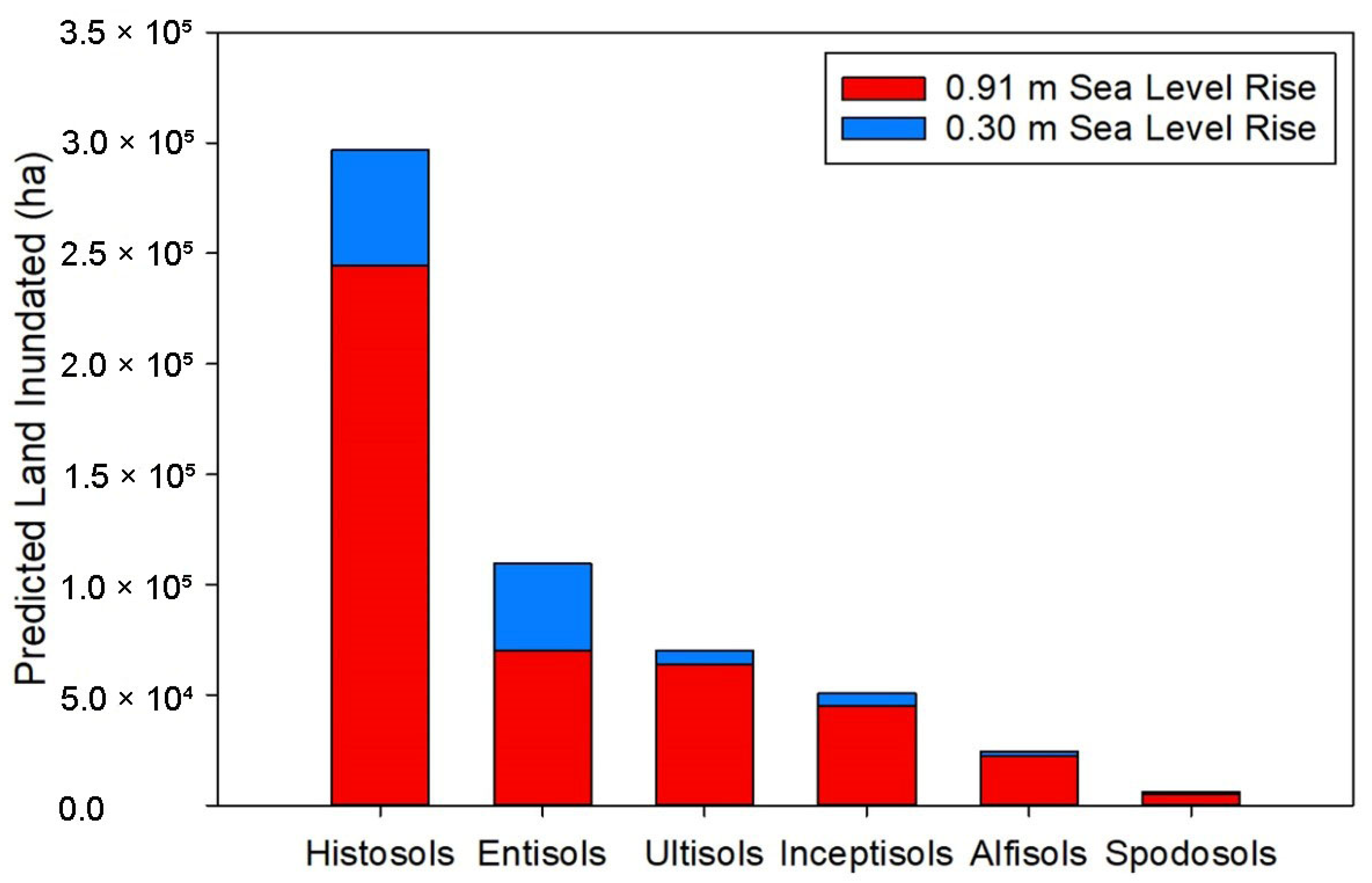
3.1. NRCS Pedon Data and Sea Level Rise

Soil data were obtained from the Soil Survey Geographic Database (SSURGO), and the North Carolina shoreline was obtained from the National Oceanic and Atmospheric Administration (NOAA) Continually Updated Shoreline Product (CUSP). The CUSP was buffered 500 m to represent the estuarine shoreline study area. Soil physical and chemical pedon data of the soil series mapped (n = 147) within this area were obtained from the National Cooperative Soil Survey (NCSS) Soil Characterization Database [27].

Under an intermediate global mean sea level rise scenario, the National Oceanic Atmospheric Administration (NOAA) technical report predicts sea levels to rise 0.30 m by 2050 and 0.91 m by 2100 [28]. Sea level rise projections were downloaded from the NOAA Office for Coastal Management web mapping tool for 0.30 and 0.91 m of sea level rise [3]. The SSURGO soils data were intersected with each sea level rise scenario and then dissolved to the taxonomic soil order to calculate hectares of each soil order covered by 0.30 (1 ft.) and 0.91 (3 ft.) meters of sea level rise.

3.2. GIS Mapping of Salinity

An average water salinity gradient was created for the APES using the Water Quality Portal (WGP), a cooperative service sponsored by the United States Geological Survey (USGS), the Environmental Protection Agency (EPA), and the National Water Quality Monitoring Council (NWQMC). We acquired the mean, maximum, and minimum salinity levels for individual water quality monitoring stations across a 10-year period from 2010 to 2019. To fill large spatial data gaps existing in the Pamlico Sound, surface water salinity was obtained in Hyde County using a handheld YSI Professional Series meter (n = 4) in 2019–2020. These salinity metrics were added to ArcGIS Pro (version 3.2, ESRI, Redlands, CA, USA) and used with the Radial Basis Functions tool. A spline with tension was applied to the water quality monitoring station points (n = 59) to create a continuous raster for the APES. The interpolated salinity values were grouped into four classes after [26]: tidal fresh (<0.5 ppt), oligohaline (0.5–5 ppt), mesohaline (5–18 ppt), and polyhaline (18–30 ppt).

3.3. Calculating Fetch

Wind data were downloaded from the NOAA Local Climatological Data Map and used to calculate fetch in the APES. Wind direction frequency was summarized in 36 directions, starting at 0 degrees (north) and proceeding clockwise in 10-degree increments for the years 2000–2019 for 8 different wind stations (Figure 1). To process the wind data in GIS, a land–water mask was created, and theissen polygons were built around each wind station to guide the delineation of fetch regions in the water. The theissen polygons were used as a guideline but modified to fit the unique geometry of the APES.

Effective fetch (EF) was then calculated for each region of the APES and 36 wind directions using tools developed by Finlayson, which implements methods from the Shore Protection Manual (SPM) and ESRI ArcGIS [29,30]. The USGS Upper Midwest Environmental Sciences Center updated these tools to operate with ArcGIS 10.x [31]. The SPM method estimates EF by calculating the arithmetic mean of nine radial measurements around the desired wind direction at 3-degree increments. This step resulted in multiple raster files for each wind direction bin and APES region, which were then weighted by the frequency that wind blew in that direction. Each region raster was merged to create a continuous layer where each grid cell value was the sum of the distance in meters to shore along each input direction weighted by the percent frequency that the wind blew from that direction.

3.4. Calculating Shoreline Erosion Rates

The USGS Earth Explorer engine was utilized to download Landsat images for the years 2000 and 2020. The shoreline for each year was traced to create a polyline to measure the shoreline change over 20 years. Using SSURGO data, 33 representative wetland map units were selected (11 Typic (deep) Histosols, 11 Terric (shallow) Histosols, and 11 mineral soils). The distance between historical and 2020 shorelines was measured in ArcGIS 5 times per soil map unit for a total of 165 measurements within the APES. The ecological state of each soil map unit was also determined (freshwater forest, ghost forest, or marsh) along with classifying the map unit as either “Open” or “Protected” from wind-driven waves. Based on the landscape position of each site, a fetch of 1500 m was chosen as the cutoff between the categories of “open” or “protected” shoreline [19].

To calculate total land loss due to erosion, Landsat images (1984, 1990, 1995, 2005, 2011, 2016, 2020) were extracted from the USGS Earth Explorer interface. The images were taken from May to September to capture peak vegetation. The bands of the satellite images were manipulated to create the greatest contrast between the land and water interface with the most common band setting with Red: Band 1, Green: Band 2, and Blue being Band 3 or 4. Once an ideal contrast was generated, a Normalized Difference Vegetation Index (NDVI) was used in ESRI ArcGIS Pro to differentiate between water and land. Manual corrections and corresponding masking of interchangeable raster values were necessary for exposed agricultural land and waterfowl impoundments.

Once the NDVI was generated for land versus water, the difference in raster area was calculated for each image regarding total land loss across the peninsula. Sequentially, the total difference between land in 1984 and 2020 was calculated using the Clip tool in ESRI ArcGIS Pro. The Clip tool was used to calculate the hectarage of each soil series lost to submergence as well as its corresponding ecosystem type (tidal forest, ghost forest, tidal marsh). Quality control was performed manually by pinpointing failed NDVI differentiations and recalculating imagery and raster values at those locations.

3.5. Field and Laboratory Data Collection

Sampling occurred in the summer of 2020. Sampling points were located in the field using a handheld Garmin GPSMap 78s. Twelve sites were sampled consisting of one transect per site with the exception of Palmetto–Peartreee (PP-GF) where two transects were completed due to site soil variability. The 20 m transect began at the open water edge and was flagged every 5 m moving inland. Five measurements of peat and sediment overwash thickness was recorded every 5 m along each transect (n = 260) using a hand-held peat probe. At the end of the 20 m transect, a MaCaulay peat auger (5 cm diameter) was used to describe and sample soils by horizon to 2 m. Soils were described using standard methods [32] and classified using the Keys to Soil Taxonomy 12th edition [33]. The von Post Humification scale was used to determine the degree of decomposition in organic horizons [34]. Bulk density samples of known volume were collected for each horizon from the MaCaulay auger (5 cm half core) or bulk density ring (5 × 5 cylinder). Bulk horizon samples were collected and placed on ice in a cooler for transport to the laboratory.

Samples from each soil horizon were analyzed for pH using 1:1 deionized (DI) water solution and 1:2 calcium chloride (CaCl₂) solution as well as 16-week aerobic incubation pH for the determination of sulfidic materials. Electrical conductivity (EC) was also analyzed for each horizon using 1:1 and 1:5 volumetric soil to deionized water solution ratios [33]. Bulk density was determined using the soil core method, and the soil texture of mineral horizons was determined via hydrometer and wet sieved sand fractionations [35,36].

Standing live and dead trees (defined as diameter at breast height (DBH) > 7.6 cm) were quantified as stems/ha within a 20 × 20 m (0.04 ha) plot around the soil sampling location. Abundance by areal cover of shrubs/saplings (<7.6 cm DBH) and herbaceous vegetation was estimated on a smaller 3 × 3 m plot adjacent to the soil sampling location [37]. All live plants were classified to the species level where possible.

3.6. Statistical Analysis

All statistical analyses were conducted in SAS (version 9.4, SAS Institute, Cary, NC, USA). Regressions were used to evaluate relationships between rates of shoreline change and fetch and between soil EC, soil pH, soil salinity, and water salinity. A one-way ANOVA was used to test the differences in shoreline change rates between ecosystems (fresh forest, ghost forest, marsh), soil types (Typic/Terric Histosols, and mineral soils), and fetch categories (open or protected). A two-way 3 × 3 ANOVA was used to test significant differences in shoreline change rates between ecosystems and soil types. A one-way ANOVA was also used to test differences between soil EC and soil porewater salinity values between ecosystems. Tukey’s HSD was used for post hoc analysis when ANOVA was significant. Significance level was set to α = 0.05 for all tests.

4. Results

4.1. Coastal Soil Survey Mapping and Study Wetland Ecosystems

There are 147 mapped soil series within 500 m of the tidal coastline of North Carolina, covering 400,635 ha. The soil orders from most hectares mapped to least are Histosols, Ultisols, Entisols, Inceptisols, Alfisols, and Spodosols, covering 32%, 28%, 25%, 7.5% 4.5%, and 3%, respectively. Of the 147 mapped series, 12 were Histosols (organic soils), 71 were aquic mineral (wetland) soils, and 64 were udic mineral (upland) soils. Major land uses of the upland mineral classes were cultivated cropland and forestry. Major land uses of the aquic mineral classes were mostly woodland with some cultivated crops or wetland wildlife habitat. Undrained coastal Histosols were all wetland wildlife habitat with the majority being Typic Haplosaprists (77% deep organic deposits > 130 cm thickness), and the remaining were Terric Haplosaprists (23% shallow organic deposits 40–130 cm thickness).

In North Carolina, NOAA sea level rise projections show Histosols will be disproportionately affected, with 244,404 ha being inundated with 0.91 m of sea level rise. Even 0.30 m of sea level rise will inundate 106,268 ha of land in North Carolina with 49.3% of that land area being Histosols (52,394 ha) (Figure 2). In our study, we quantified the ecosystem parameters for 12 representative coastal wetlands mapped as Histosols (cumulative peat thickness > 40 cm). There were four coastal tidal forests, four ghost forests, and four tidal marshes along a longitudinal salinity gradient (

Table 1. Table showing each field study site, ecosystem salinity level, peat depth, and dominant plant species.

Site	Mean Salinity (ppt)	Mean Peat Thickness (cm)	Live Trees (Stems/ha)	Dead Trees (Stems/ha)	Dominant Trees a	Dominant Shrubs/Saplings b	Dominant Emergents b
Tidal Forest Sites
CR-CF	0.15	250+	550	25	Nyssa biflora (73.7%) Taxodium distichum (10.5%)	Carpinus caroliniana (15%) Clethra alnifolia (10%)	Polygonum spp. (30%) Osmunda regalis (10%)
TR-CF	0.22	250+	675	25	Nyssa aquatica (85.2%) T. distichum (7.4%)	Fraxinus pennsylvanica (20%) Acer rubrum (10%)	Persicaria arifolia (20%) O. regalis (10%)
BN-CF	1.10	206	675	25	N. aquatica (81.5%) T. distichum (7.4%)	Morella cerifera (35%) Persea borbonia (10%)	Pontederia cordata (20%) O. regalis (15%)
RR-CF	1.61	250+	700	25	N. aquatica (60.7%) N. biflora (17.9%)	F. pennsylaniva (15%) A. rubrum (10%)	Carex spp. (30%) Cicuta maculate (5%)
Ghost Forest Sites
AR-GF	3.51	230	275	325	N. aquatica (90.9%) Pinus taeda (9.1%)	P. borbonia (10%) Pinus taeda (10%)	Cladium jamaicense (60%) Phragmites australis (10%)
PP-GF	4.38	69	63	238	P. taeda (40.0%) N. aquatica (40.0%)	M. cerifera (10%) A. rubrum (5%)	P. australis (95%) Toxicodendron radicans (5%)
BH-GF	5.36	116	0	350	N/A	Chamaecyparis thyoides (15%) P. taeda (5%)	C. jamaicense (75%) Juncus roemerianus (10%)
GC-GF	8.28	112	0	100	N/A	N/A	Bolboschoenus robustus (90%) Spartina cynosuroides (5%)
Tidal Marsh Sites
LR-TM	11.73	116	0	0	N/A	N/A	S. cynosuroides (50%) J. roemerianus (40%)
SQ-TM	13.67	201	0	0	N/A	N/A	J. roemerianus (80%) B. robustus (10%)
JB-TM	15.39	172	0	0	N/A	N/A	J. roemerianus (85%) Spartina alterniflora (5%)
PP-TM	15.47	194	0	0	N/A	N/A	C. jamaicense (70%) P. australis (5%)

^a Measured as a percent of total stems/ha within study plots. ^b Measured as areal abundance within study plots.

). Tidal forests ranged from 0.15 to 1.61 ppt salinity and were dominated by water tupelo (Nyssa aquatica L.) and swamp tupelo (Nyssa biflora Walter) with baldcypress (Taxodium distichum L. (Rich.)) present at most sites. Tree density ranged from 550 to 700 stems/ha, and site soils were deep Histosols (>200 cm peat thickness).

As site salinity increased, we observed overstory tree mortality within ghost forests at 3.51 ppt, and no live trees were observed at sites >5.36 ppt. Ghost forests with live trees were dominated by water tupelo and loblolly pine (Pinus taeda L.), but density was <275 stems/ha. Standing dead trees increased to 100–350 stems/ha within ghost forests, and the areal abundance of emergent plants increased significantly. Salt-tolerant oligohaline species like sawgrass (Cladium mariscus (L.) Pohl ssp. jamaicense (Crantz) Kük.), invasive common reed (Phragmites australis (Cav.) Trin. ex Steud.), and sturdy bulrush (Bolboschoenus robustus (Pursh) Soják) were present in the understory of our study plots. Peat thickness was highly variable in ghost forests but was shallower than tidal forests ranging from 69 to 230 cm (Table 1).

Tidal marshes in this study were all mesohaline, ranging from 11.73 to 15.47 ppt. The dominant emergent species were salt-tolerant black needlerush (Juncus roemerianus Scheele) and big cordgrass (Spartina cynosuroides (L.) Roth). The PP-TM site was dominated by sawgrass because of the extensive freshwater influx from groundwater seeps around the study plots, which prevented more salt-tolerant species like black needlerush from dominating this mesohaline marsh site. There were no standing trees or woody shrubs present within any of the study site marshes, and the soil peat thickness was less variable than ghost forests, ranging from 116 to 201 cm (Table 1).

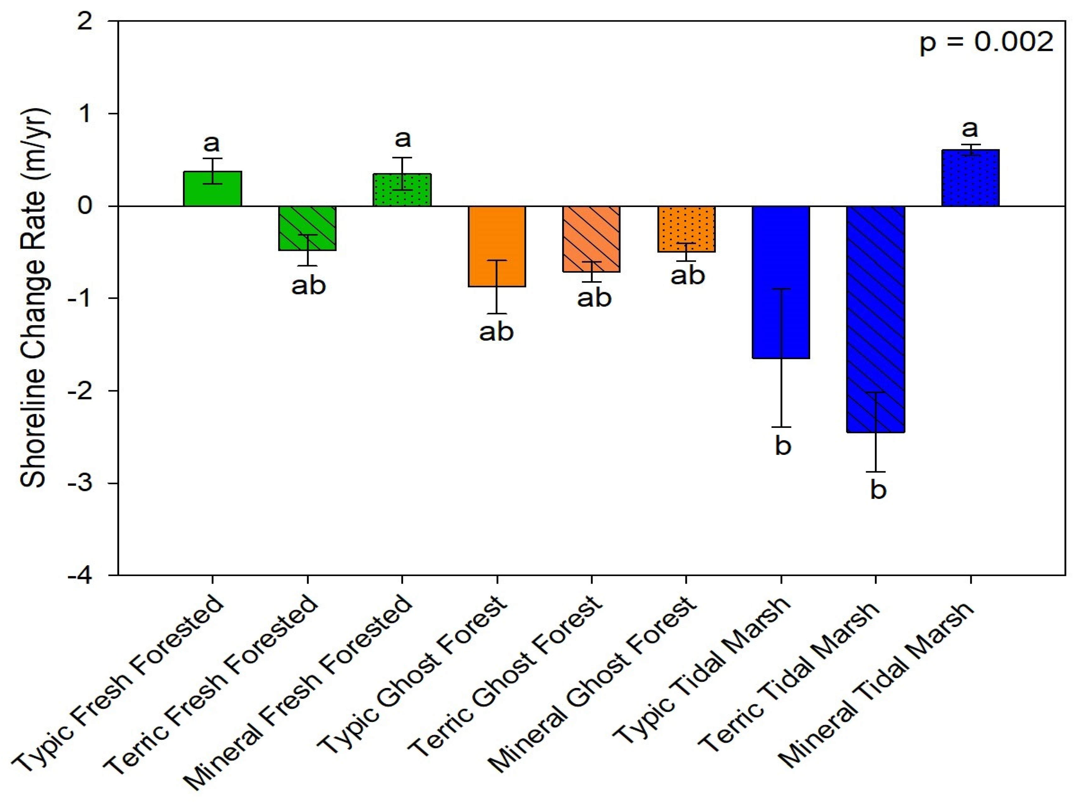
4.2. Fetch and Ecosystem Erosion Rates

Fetch was the highest along the long axis of the Pamlico Sound and lowest in the Chowan and Tar Rivers (Figure 1). The PP-GF site had the highest fetch at 14,430 m, and BH-GF had the lowest fetch at 424 m. The four sites considered protected with a fetch less than 1500 m were BH-GF, TR-CF, JB-TM, and CR-CF. All other research sites were considered open shorelines with fetches larger than 1500 m. The fetch and shoreline change rate for 33 representative soil map units selected are significantly related (r² = 0.15, p = 0.02, Figure 3).

The shoreline change rate of the APES ranged from accretion of +1.04 m/yr to erosion of −7.18 m/yr. The average shoreline rate of change (m/yr) was significantly different among ecosystems (p = 0.004), soil type (p < 0.001), and fetch category (p < 0.001) (

Table 2. ANOVA table for the main effect of ecosystem, soil type, and fetch and their interactions on the average m/yr shoreline change. Different letters indicate significant differences within the ecosystem, type, and fetch category (α = 0.05).

Ecosystem × Soil Type		p = 0.002
Ecosystem × Fetch		p = 0.001
Soil Type × Fetch		p = 0.26
Ecosystem	n	Average m/yr	Significance (p = 0.004)
Freshwater	40	0.26	a
Ghost Forest	70	−0.65	b
Marsh	55	−1.60	c
Soil Type	n	Average m/yr	Significance (p < 0.001)
Typic	55	−0.70	a
Terric	55	−1.48	b
Mineral	55	−0.07	a
Fetch	n	Average m/yr	Significance (p < 0.001)
Open	115	−1.18	a
Protected	50	0.23	b

). Freshwater tidal forested wetlands were the only ecosystem to be net accreting (mean 0.26 ± 0.11 m/yr), while ghost forests (−0.65 ± 0.08) and marshes (−1.60 ± 0.36) were net eroding. Terric Histosol map units had an average −1.48 ± 0.20 m/yr shoreline change rate, which was significantly higher than the mean shoreline change rate of Typic Histosol map units (0.70 ± 0.10 m/yr) and mineral hydric soil map units (0.07 ± 0.01 m/yr). Sites considered to have an open fetch also had an average shoreline change rate of −0.17 ± 0.19 m/yr, which was significantly different from protected sites that were net accreting (0.23 ± 0.10 m/yr).

The interaction between ecosystem and fetch category was significant (p = 0.001) (Figure 4). Open tidal marshes were eroding at a significantly higher rate than all other shoreline variations. The interaction between ecosystem and soil type was also significant (p = 0.002). Regardless of soil type, ghost forests were eroding at a similar rate. Terric soil map units across all three ecosystems were eroding, while mineral and Typic soil map units in freshwater forested wetlands were accreting. In marshes, the mineral soil map units were accreting, but Terric and Typic soil map units were eroding (Figure 5).

Landsat and NDVI data analysis from 1984 to 2020 indicated a total of 2833 ha of land has been submerged in the Albemarle–Pamlico Sound due to sea level rise with the majority (91.6%) of this loss coming from tidal marsh and ghost forest ecosystems (Figure 6). Net land loss was similar to rates calculated among coastal ecosystems, showing that lower estuary ecosystems are net erosional compared to upper estuary forested ecosystems that promote accretion and low net shoreline erosion rates over time regardless of fetch or soil type (Figure 4 and Figure 5).

5. Discussion

Soil Survey Histosol Mapping and Erosion Rates

Although nearly 95% of the soils in the U.S. are mapped and available on the Web Soil Survey, many coastal zone areas have not been mapped sufficiently to provide the interpretive data necessary for effective coastal land management. The knowledge and accurate mapping of coastal zone soils is extremely important, considering 40% of the United States’ population live in coastal counties [3]. Soils mapped in coastal wetlands have always provided valuable wildlife habitat, but we now recognize additional ecosystem services such as carbon sequestration, flood and storm surge protection, and nutrient filtering in these landscapes [2]. For example, coastal wetlands accumulate C at rates 1 to 2 orders of magnitude greater than terrestrial systems and are important components within the global C budget [38,39]. Improved understanding of these “blue carbon” ecosystems is critical to managing coastal wetlands in the face of climate change and predicted sea level rise [39].

In the APES, several factors including fetch, nearshore bathymetry, shoreline morphology and vegetation community have all been shown to influence shoreline rates of change [7]. Shorelines were found to have variable rates of change dependent on fetch, shoreline ecosystem, or soil map unit type. The 20-year average rate of shoreline change for all of the soil map units measured throughout the APES was −0.75 m/yr. This is comparable with previous studies of estuarine shorelines in North Carolina [7,10,40,41]. We found the tidal freshwater forested wetlands (Chowan, Roanoke, Tar Rivers) were on average accreting, while the ghost forests and marshes in the APES were net eroding. Most alluvial sediment enters the estuary through the freshwater tributary rivers and is deposited in these areas of the upper estuary. In addition, the lower Chowan and Roanoke Rivers consist of organic deposits that have been accumulating for the last 5000 years at mean rates of 0.15 cm/yr [42]. Natural accretion in the fluvial deltaic landscape positions helps offset shoreline erosion within the upper estuary, but the lack of alluvial sediment entering tidal marshes throughout most of the eastern APES results in sediment-starved shorelines [19]. The eastern APES is also generally characterized by larger fetches, higher energy waves, and more frequent storm tide conditions resulting in higher net erosion rates [7,10].

Ghost forests were all found to be eroding at similar rates regardless of soil type. This is likely due to the unstable shoreline as trees die off and the vegetation shifts to a more salt-tolerant marsh community. Before salt-tolerant plants become established, the soil is more vulnerable to physical erosion because plant roots can reduce erosion by stabilizing sediments and exposed banks [43,44]. This conversion from freshwater forested wetland to marsh can take over a decade or more, resulting in increased erosion throughout the transition period [1,45].

We found marshes to have the highest net erosion rate between the three ecosystems, even though marshes are known to be relatively difficult to erode due to their cohesive sediments, binding roots, and ability to vertically accrete through sediment and organic matter accumulation [46,47]. However, the limited sediment supply in much of the APES requires high organic matter production as the dominant mechanism of vertical accretion [48]. Between marsh types, mineral tidal marshes were found to be net accreting, while both Terric and Typic Histosol marshes were eroding. This is consistent with previous findings that indicate the higher bulk density in mineral soils decreases wave-driven erodibility when compared to low bulk density organic soils [49,50].

Of our 33 soil map units measured in our study, the linear relationship between shoreline change rates and fetch explains only 15% of the variation in the data, although low fetch values generally have net accretion, and high fetch values are correlated to more net erosion (p = 0.02). The fetch data range used to calculate this relationship was from <100 to 15,000 m which represents the range of all shorelines within the greater APES. Although the data used in our study are heterogeneous and represent mostly fetch values < 5000 m, other regional studies have shown similar relationships between fetch and shoreline change. For example, [40] found that the linear relationship between shoreline change rates and fetch only explained 15% of the variation in their APES data as well. In their study, the majority of shoreline points (95%) with a mean fetch value greater than 1500 m were eroding, while we found 72% at sites with similar conditions [40]. In the micro-tidal APES, waves have been identified as an important mechanism for shoreline change. Although we did not simulate waves in this study, shoreline orientation, wind speed and direction, as well as local bathymetry are important in determining wave energy with wave heights being greatest in areas where shoreline orientation and wind direction resulted in the most exposure [51]. Future wave modeling research within the APES is needed to improve our current understanding of how spatially complex bathymetry, wind, and shoreline factors that influence shoreline change.

6. Conclusions

The results from this work investigate soils of the North Carolina coastal zone providing information on erosion and accretion rates for different soils and ecosystems. Our data show that tidal marsh and ghost forest landscapes within the APES have been eroding at higher rates than freshwater forested ecosystems. Net accretion is the greatest in tidal forests that are protected from wind and wave action at the shoreline edge. This study provides a framework to update and create new, more accurate, soil surveys of coastal zone wetlands that will allow for collaborative research efforts across disciplines. However, more effort is needed to reevaluate ghost forest and marsh landscapes within the APES for targeted mitigation activities to slow shoreline erosion (e.g., thin layer deposition, living shorelines). In the future, combined soil and ecosystem-level predictions of shoreline change will improve our ability to respond to complex coastal issues, as these areas impacted by sea level rise undergo rapid transformations.

References

1. White, E.; Kaplan, D. Restore or Retreat? Saltwater Intrusion and Water Management in Coastal Wetlands. Ecosyst. Health Sustain. 2017, 3, e01258. [Google Scholar] [CrossRef]
2. Barbier, E.B.; Hacker, S.D.; Kennedy, C.; Koch, E.W.; Stier, A.C.; Silliman, B.R. The Value of Estuarine and Coastal Ecosystem Services. Ecol. Monogr. 2011, 81, 169–193. [Google Scholar] [CrossRef]
3. National Oceanic and Atmospheric Administration (NOAA) Office for Coastal Management. Sea Level Rise Viewer. 2021. Available online: https://maps.coast.noaa.gov/digitalcoast/tools/slr.html (accessed on 1 May 2021).
4. Deaton, A.S.; Chappell, W.S.; Hart, K.; O’Neal, J.; Boutin, B. North Carolina Coastal Habitat Protection Plan; North Carolina Department of Environment and Natural Resources, Division of Marin Fisheries: Morehead City, NC, USA, 2010. [Google Scholar]
5. McVerry, K. North Carolina Estuarine Shoreline Mapping Project: Statewide and County Statistics; North Carolina Division of Coastal Management: Morehead City, NC, USA, 2012; pp. 1–145. [Google Scholar]
6. Corbett, D.R.; Walsh, J.P.; Cowart, L.; Riggs, S.R.; Ames, D.V.; Culver, S.J. Shoreline Change within the Albe-Marle-Pamlico Estuarine System, North Carolina; East Carolina University: Greenville, NC, USA, 2008. [Google Scholar]
7. Cowart, L.; Corbett, D.R.; Walsh, J.P. Shoreline Change along Sheltered Coastlines: Insights from the Neuse River Estuary, NC, USA. J. Remote Sens. 2011, 3, 1516–1534. [Google Scholar] [CrossRef]
8. National Research Council. Mitigating Shore Erosion along Sheltered Coasts; The National Academies Press: Washington, DC, USA, 2007. [Google Scholar]
9. Bellis, V.; O’Conner, M.P.; Riggs, S.R. Estuarine Shoreline Erosion in the Albemarle Pamlico Region of North Carolina; UNC Sea Grant Publication, North Carolina State University: Raleigh, NC, USA, 1975. [Google Scholar]
10. Riggs, S.R.; Ames, D.P. Drowning the North Carolina Coast: Sea-Level Rise and Estuarine Dynamics; North Carolina Sea Grant: Raleigh, NC, USA, 2003. [Google Scholar]
11. Luettich, R.A.; Carr, S.D.; Reynolds-Fleming, J.V.; Fulcher, C.W.; McNinch, J.E. Semi-Diurnal Seiching in a Shallow, Micro-Tidal Lagoonal Estuary. Cont. Shelf Res. 2002, 22, 1669–1681. [Google Scholar] [CrossRef]
12. Eulie, D.O. Examination of Estuarine Sediment Dynamics: Insights from the Large, Shallow, Albemarle-Pamlico Estu-Arine System, NC, U.S.A. Ph.D. Thesis, East Carolina University, Greenville, NC, USA, 2014. [Google Scholar]
13. Day, J.W.; Christian, R.R.; Boesch, D.M.; Yáñez-Arancibia, A.; Morris, J.; Twilley, R.R.; Naylor, L.; Schaffner, L.; Stevenson, C. Consequences of Climate Change on the Ecogeomorphology of Coastal Wetlands. Estuaries Coasts 2008, 31, 477–491. [Google Scholar] [CrossRef]
14. Ury, E.A.; Yang, X.; Wright, J.P.; Bernhardt, E.S. Rapid Deforestation of a Coastal Landscape Driven by Sea-Level Rise and Extreme Events. Ecol. Appl. 2021, 31, e02339. [Google Scholar] [CrossRef] [PubMed]
15. Helton, A.M.; Ardon, M.; Bernhardt, E.S. Hydrologic context alters greenhouse gas feedbacks of coastal wetland salinization. Ecosystems 2019, 22, 1108–1125. [Google Scholar] [CrossRef]
16. Kirwan, M.L.; Gedan, K.B. Sea-Level Driven Land Conversion and the Formation of Ghost Forests. Nat. Clim. Chang. 2019, 9, 450–457. [Google Scholar] [CrossRef]
17. Smart, L.S.; Taillie, P.J.; Poulter, B.; Vukomanovic, J.; Singh, K.K.; Swenson, J.J.; Mitasova, H.; Smith, J.W.; Meentemeyer, R.K. Aboveground Carbon Loss Associated with the Spread of Ghost Forests as Sea Levels Rise. Environ. Res. Lett. 2020, 15, 104028. [Google Scholar] [CrossRef]
18. Jia, P.; Li, M. Circulation Dynamics and Salt Balance in a Lagoonal Estuary. J. Geophys. Res. 2012, 117, 1–16. [Google Scholar] [CrossRef]
19. Giese, G.L.; Wider, H.B.; Parker, G.G., Jr. Hydrology of Major Estuaries and Sounds of North Carolina. In US Geological Survey Water Supply Paper; USGS: Reston, VA, USA, 1985; Volume 108. [Google Scholar]
20. Ingram, R.L. Peat Deposits of North Carolina, Bulletin 88; North Carolina Department of Natural Resources and Community Development: Raleigh, NC, USA, 1987; pp. 1–84. [Google Scholar]
21. Henman, J.; Poulter, B. Inundation of Freshwater Peatlands by Sea Level Rise: Uncertainty and Potential Carbon Cycle Feedbacks. J. Geophys. Res. Biogeosci. 2008, 113, 1–11. [Google Scholar] [CrossRef]
22. Soil Survey Staff. Web Soil Survey; USDA-NRCS: Washington, DC, USA, 2019. [Google Scholar]
23. Rabenhorst, M.C.; Stolt, M.H. Chapter 6—Subaqueous Soils: Pedogenesis, Mapping, and Applications. In Hydropedology; Academic Press: Cambridge, MA, USA, 2012. [Google Scholar]
24. Ardon, M.; Morse, J.L.; Colman, B.P.; Bernhardt, E.S. Drought-Induced Saltwater Incursion Leads to Increased Wetland Nitrogen Export. Glob. Chang. Biol. 2013, 19, 2976–2985. [Google Scholar] [CrossRef] [PubMed]
25. Manda, A.K.; Giuliano, A.S.; Allen, T.R. Influence of Artificial Channels on the Source and Extent of Saline Water Intrusion in the Wind Tide Dominated Wetlands of the Southern Albemarle Estuarine System. Environ. Earth Sci. 2014, 71, 4409–4419. [Google Scholar] [CrossRef]
26. Cowardin, L.M.; Carter, V.; Golet, F.C.; LaRoe, E.T. Classification of Wetlands and Deepwater Habitats of the United States; U.S. Government Printing Office: Washington, DC, USA, 1979. [Google Scholar]
27. National Cooperative Soil Survey, National Cooperative Soil Characterization Database 2023. Available online: http://ncsslabdatamart.sc.egov.usda.gov/ (accessed on 1 August 2023).
28. Sweet, W.V.; Hamlington, B.D.; Kopp, R.E.; Weaver, C.P.; Barnard, P.L.; Bekaert, D.; Brooks, W.; Craghan, M.; Dusek, G.; Frederikse, T.; et al. Global and Regional Sea Level Rise Scenarios for the United States: Updated Mean Projections and Extreme Water Level Probabilities Along U.S. Coastlines; National Oceanic and Atmospheric Administration, National Ocean Service: Silver Spring, MD, USA, 2022; p. 111. [Google Scholar]
29. Finlayson, D. Puget Sound Fetch: Seattle, Washington; University of Washington, School of Oceanography: Seattle, WA, USA, 2005. [Google Scholar]
30. USACE. Shore Protection Manual; Coastal Engineering Research Center: Fort Belvoir, VA, USA, 1984. [Google Scholar]
31. Rohweder, J.; Rogala, J.T.; Johnson, B.L.; Anderson, D.; Clark, S.; Chamberlin, F.; Potter, D.; Runyon, K. Application of Wind Fetch and Wave Models for Habitat Rehabilitation and Enhancement Projects—2012 Update; United States Geological Survey: Reston, VA, USA, 2012. [Google Scholar]
32. Schoeneberger, P.J.; Wysocki, D.A.; Benham, E.C.; Staff, S.S. Field Book for Describing and Sampling Soils, Version 3.0; Natural Resources Conservation Service, National Soil Survey Center: Lincoln, NE, USA, 2012. [Google Scholar]
33. Soil Survey Staff. Keys to Soil Taxonomy, 12th ed.; U.S. Government Printing Office: Washington, DC, USA, 2014. [Google Scholar]
34. Von Post, L.; Granlund, E. Peat resources in southern Sweden. Sver. Geol. Undersökning Yearb. 1926, 335, 1–127. [Google Scholar]
35. Blake, G.R.; Hartge, K.H. Bulk Density, 2nd ed.; Klute, A., Ed.; American Society of Agronomy/Soil Science Society of America: Madison, WI, USA, 1986. [Google Scholar]
36. Gee, G.W.; Bauder, J.W. Particle Size Analysis, 2nd ed.; Klute, A., Ed.; American Society of Agronomy/Soil Science Society of America: Madison, WI, USA, 1986. [Google Scholar]
37. USACE; Wakeley, J.S.; Lichvar, R.W.; Noble, C.V. Regional Supplement to the Corps of Engineers Wetland Delineation Manual: Atlantic and Gulf Coastal Plain Region. U.S. Army Engineer Research and Development Center: Vicksburg, MS, USA, 2010. [Google Scholar]
38. Chmura, G.L.; Anisfeld, S.C.; Cahoon, D.R.; Lynch, J.C. Global carbon sequestration in tidal, saline wetland soils. Glob. Biogeochem. Cycles 2003, 17. [Google Scholar] [CrossRef]
39. McLeod, E.; Chmura, G.L.; Bouillon, S.; Salm, R.; Björk, M.; Duarte, C.M.; Lovelock, C.E.; Schlesinger, W.H.; Silliman, B.R. A Blueprint for Blue Carbon: Toward an Improved Understanding of the Role of Vegetated Coastal Habitats in Sequestering CO2. Front. Ecol. Environ. 2011, 9, 552–560. [Google Scholar] [CrossRef] [PubMed]
40. Cowart, L.; Walsh, J.P.; Corbett, D.R. Analyzing estuarine shoreline change: A case study of Cedar Island, North Carolina. J. Coast. Res. 2010, 26, 817–830. [Google Scholar] [CrossRef]
41. Eulie, D.O.; Walsh, J.P.; Corbett, D.R.; Mulligan, R.P. Temporal and Spatial Dynamics of Estuarine Shoreline Change in the Albemarle-Pamlico Estuarine System, North Carolina, USA. Estuaries Coasts 2017, 40, 741–757. [Google Scholar] [CrossRef]
42. Wells, J.T.; Kim, S.Y. Sedimentation in the Albemarle-Pamlico Lagoonal System: Synthesis and Hypotheses. Mar. Geol. 1989, 88, 263–284. [Google Scholar] [CrossRef]
43. Le Hir, P.; Monbet, Y.; Orvain, F. Sediment Erodibility in Sediment Transport Modelling: Can We Account for Biota Effects? Cont. Shelf Res. 2007, 27, 1116–1142. [Google Scholar] [CrossRef]
44. Turner, R.E. Beneath the Salt Marsh Canopy: Loss of Soil Strength with Increasing Nutrient Loads. Estuaries Coasts 2011, 34, 1084–1093. [Google Scholar] [CrossRef]
45. Craft, C.B. Tidal Freshwater Forest Accretion Does Not Keep Pace with Sea Level Rise. Glob. Chang. Biol. 2012, 18, 3615–3623. [Google Scholar] [CrossRef]
46. Craft, C.B.; Seneca, E.D.; Broome, S. Vertical Accretion in Microtidal Regularly and Irregularly Flooded Estuarine Marshes. Estuar. Coast. Shelf Sci. 1993, 37, 371–386. [Google Scholar] [CrossRef]
47. Pierfelice, K.N.; Graeme Lockaby, B.; Krauss, K.W.; Conner, W.H.; Noe, G.B.; Ricker, M.C. Salinity Influences on Aboveground and Belowground Net Primary Productivity in Tidal Wetlands. J. Hydrol. Eng. 2017, 22, D5015002. [Google Scholar] [CrossRef]
48. Moorhead, K.K.; M, B.M. Response of Wetlands to Rising Sea Level in the Lower Coastal Plain of North Carolina. Ecol. Appl. 1995, 5, 26–71. [Google Scholar] [CrossRef]
49. Wang, H.; Wal, D.; Li, X.; Belzen, J.; Herman, P.M.J.; Hu, Z.; Ge, Z.; Zhang, L.; Bouma, T.J. Zooming in and out: Scale Dependence of Extrinsic and Intrinsic Factors Affecting Salt Marsh Erosion. J. Geophys. Res. Earth Surf. 2017, 122, 1455–1470. [Google Scholar] [CrossRef]
50. Feagin, R.A.; Lozada-Bernard, S.M.; Ravens, T.M.; Möller, I.; Yeager, K.M.; Baird, A.H. Does Vegetation Prevent Wave Erosion of Salt Marsh Edges? National Academy of Sciences of the United States of America: Washington, DC, USA, 2009; pp. 10109–10113. [Google Scholar] [CrossRef] [PubMed]
51. Eulie, D.O.; Walsh, J.P.; Corbett, D.R. High-Resolution Analysis of Shoreline Change and Application of Balloon-Based Aerial Photography, Albemarle-Pamlico Estuarine System, North Carolina, USA. Limnol. Oceanogr. 2013, 11, 151–160. [Google Scholar] [CrossRef]
Figure 1. Map of the 33 map units where shoreline change rates were calculated (field site labels correspond to Table 1) with wind stations and weighted wind fetch in meters. Prevailing winds come from the southwest or northeast, aligning with the long axis of the Pamlico Sound generating a large fetch. Fetch decreases in the Albemarle Sound and up the microtidal rivers.
Forests 15 01069 g001
Figure 2. Graph showing hectares inundated in North Carolina of different soil orders for 0.30 and 0.91 m of sea level rise scenarios [3,28].
Forests 15 01069 g002
Figure 3. Linear regression (red line) between shoreline change rates and fetch for the 33 soil map units selected. Gray lines represent 95% confidence interval. Positive values represent net accretion versus negative values that represent net shoreline erosion. Outlier data points with the greatest net erosion rates are from Point Peter, which is a low-elevation tidal marsh that has been anthropogenically modified via ditching which contributes to increased shoreline erosion in this area [10].
Forests 15 01069 g003
Figure 4. Graph showing average rate of shoreline change in the three ecosystems and fetch categories with standard error bars. Different letters indicate significant differences (α = 0.05).
Forests 15 01069 g004
Figure 5. Graph showing average rate of shoreline change for the three ecosystems and soil types with standard error bars. Typic are deep organic soils (≥130 cm peat depth) and Terric are shallow organic soils (40–130 cm peat depth). Different letters indicate significant differences (α = 0.05).
Forests 15 01069 g005
Figure 6. Graph showing total hectares submerged in the APES from 1984 to 2020 by ecosystem type.
Forests 15 01069 g006