Article

Use of a Consumer-Grade UAV Laser Scanner to Identify Trees and Estimate Key Tree Attributes across a Point Density Range

by
Michael S. Watt
1,*,
Sadeepa Jayathunga
2,
Robin J. L. Hartley
2,
Grant D. Pearse
3,
Peter D. Massam
2,
David Cajes
2,
Benjamin S. C. Steer
2 and
Honey Jane C. Estarija
2
1
Scion, 10 Kyle Street, Christchurch 8011, New Zealand
2
Scion, 49 Sala Street, Rotorua 3046, New Zealand
3
College of Science and Engineering, Flinders University, Sturt Road, Bedford Park 5042, Australia
*
Author to whom correspondence should be addressed.
Forests 2024, 15(6), 899; https://doi.org/10.3390/f15060899
Submission received: 3 May 2024 / Revised: 17 May 2024 / Accepted: 17 May 2024 / Published: 22 May 2024
(This article belongs to the Section Forest Inventory, Modeling and Remote Sensing)

Abstract

:
The management of plantation forests using precision forestry requires advanced inventory methods. Unmanned aerial vehicle laser scanning (ULS) offers a cost-effective approach to accurately estimate forest structural attributes at both plot and individual tree levels. We examined the utility of ULS data collected from a radiata pine stand for tree detection and prediction of diameter at breast height (DBH) and stem volume, using data thinned to 13-point densities (ranging from 10–12,200 points/m2). These datasets were created using a DTM with the highest pulse density and DTMs that used the native decimated point clouds. Models of DBH were constructed using partial least squares (PLS) and random forest (RF) from seven classes of metrics that characterized the horizontal and vertical structure of the canopy. Individual tree segmentation was consistently accurate across the 13-point densities and was insensitive to DTM type (F1 scores > 0.96). Predictions of DBH using PLS models were consistently more accurate than RF models and accuracy was insensitive to the DTM type. Using data from the native DTMs, DBH estimation using PLS had the lowest RMSE of 1.624 cm (R2 of 0.756) at a point density of 12,200 points/m2. Stem volume predictions made using PLS predictions of DBH and height from the ULS had the lowest RMSE of 0.0418 m3 (R2 of 0.792) at 12,200 points/m2. The RMSE values for DBH and volume remained relatively stable from 12,200 to between 750 and 400 points/m2, with reductions in accuracy occurring as point density declined below this threshold. Overall, these findings have significant implications, particularly for the precise estimation of DBH and stem volume at the individual tree level. They demonstrate the potential of cost-effective ULS sensors for rapid and frequent plantation forest assessment, thereby enhancing the application of light detection and ranging (LiDAR) technology in plantation forest management.

1. Introduction

Plantation forests cover approximately 131 million ha, constituting 3 percent of the global forest area [1]. They play a pivotal role in meeting demands for wood, fuel material, and various forest products. Additionally, they provide ecological and environmental services such as carbon sequestration [2]. Currently, New Zealand has a plantation forest area of about 1.8 million ha [3], equivalent to approximately 21 percent of its total forest cover.
These plantation areas require frequent inventory and assessment to ensure sustainable long-term management [4,5,6]. Therefore, the precise estimation of tree structural attributes is of paramount importance for forest managers, given their strong correlation with site productivity, tree growth, and commercial timber volume [7,8,9,10]. Using a plot-based system, typically Diameter at Breast Height (DBH) is measured from all trees, while height is measured from a sub-sample, and both metrics are used via volume functions to estimate total stem volume.
Traditional methods for measuring DBH and height are laborious, time-intensive, costly, subjective, and error-prone, thereby limiting scalability. In contrast, remote sensing (RS), particularly Light Detection and Ranging (LiDAR) technology, provides a convenient toolkit for in situ tree inventories. LiDAR facilitates the acquisition of detailed three-dimensional (3D) information around important structural metrics such as crown diameter, volume, height, and shape [11]. These metrics exhibit strong correlations with individual tree size [12] and can be used to accurately predict stem and tree volume at scale [13].
The adoption of LiDAR for forest inventories has increased markedly over the past few decades, which has been attributed to declining acquisition costs. However, airborne laser scanning (ALS) remains operationally complex and relatively expensive for smaller-scale applications such as stand-level assessments [14]. ALS produces relatively low-density point clouds and can be expensive to capture in small stands. Static terrestrial laser scanning (TLS) is often impractical in forestry settings due to the need for unimpeded forest access and line of sight to all trees. Using this method there are often occlusions above the canopy, resulting in inaccurate height measurements. Mobile laser scanning (MLS) backpack systems also face similar limitations to TLS, as they require users to navigate through forests and this method is prone to occlusions. Both TLS and MLS datasets captured from young, dense plantation stands are often noisy due to excessive needle leaf cover that prevents laser pulses from penetrating the stem. This makes it challenging to accurately reconstruct tree stems for direct measurements of tree attributes such as DBH.
An attractive alternative to these methods is unmanned aerial vehicle laser scanning (ULS), offering a more budget-friendly means of capturing high-density point clouds across forested areas of small to medium scale [15,16]. Recent advances in miniaturization and commercialization of low-cost, solid-state ULS have made entry costs for this technology even more affordable [17]. Consumer-grade ULS sensors, such as the DJI-Zenmuse L1 (DJI, Shenzhen, China; hereafter referred to as DJI-L1), have emerged as appealing choices for stand assessment when acquisitions need to be cost effective, rapid, and/or frequent.
Previous research has extensively investigated the use of area-averaged LiDAR variables to predict forest attributes across a wide range of ALS pulse densities [18,19,20,21]. For example, distributional metrics determined using reduced point density can provide a relatively stable level of accuracy in estimating important forest structural attributes including above-ground biomass (AGB) in tropical forests [22]. Similarly, in mixed conifer forests, the associations between ALS-derived metrics and tree attributes such as height, DBH, and basal area remained largely unaffected until the point density was reduced to very low values, i.e., below 1 point/m2 [23].
Considerable research has utilized expensive LiDAR sensors for mainly research-based applications. However, the development of commercial applications within plantation settings will largely rely on the use of inexpensive commercial-grade LiDAR sensors, such as the recently released DJI L1 sensor. Developing an understanding of the accuracy of such sensors for predicting key attributes within forests is a critical step before such sensors can be commercially deployed. It is unclear if data from these types of sensors require more intensive processing and whether the high point density provided by these sensors can be usefully utilized in the description of key forest metrics. Further research is also required to identify the parameter combinations that yield the most accurate tree characterization. In addition, little research has examined how variation in point cloud densities of data collected from commercial-grade ULS affects the accuracy of structural attribute estimation in planted forests [24].
This study collected field measurements and high-density ULS data from the commercial-grade DJI L1 sensor over a nine-year-old radiata pine (Pinus radiata D. Don) plantation. These data were used to detect and segment individual trees and estimate DBH and stem volume using decimated ULS data with 13 point densities, ranging from 10–12,200 points/m2. Datasets were created using a DTM with the highest point density (24,450 points/m2) and DTMs that used the 13 native decimated point cloud densities to examine the impact of DTM quality on detection and predictions. Two contrasting modeling approaches, that included partial least squares (PLS) and random forest (RF), were used to predict DBH from seven classes of metrics that characterized horizontal and vertical canopy structure. The most accurate predictions of DBH were then combined with height from the ULS to estimate stem volume.
Using these combinations of factors, the objectives of this study were to (i) quantify the influence of point density and DTM type on the accuracy of tree segmentation, (ii) determine the impact of model approach, point density, and DTM type on prediction accuracy for DBH, (iii) identify the most important metric class for predictions of DBH, and (iv) determine the influence of point density on the accuracy of stem volume predictions.

2. Materials and Methods
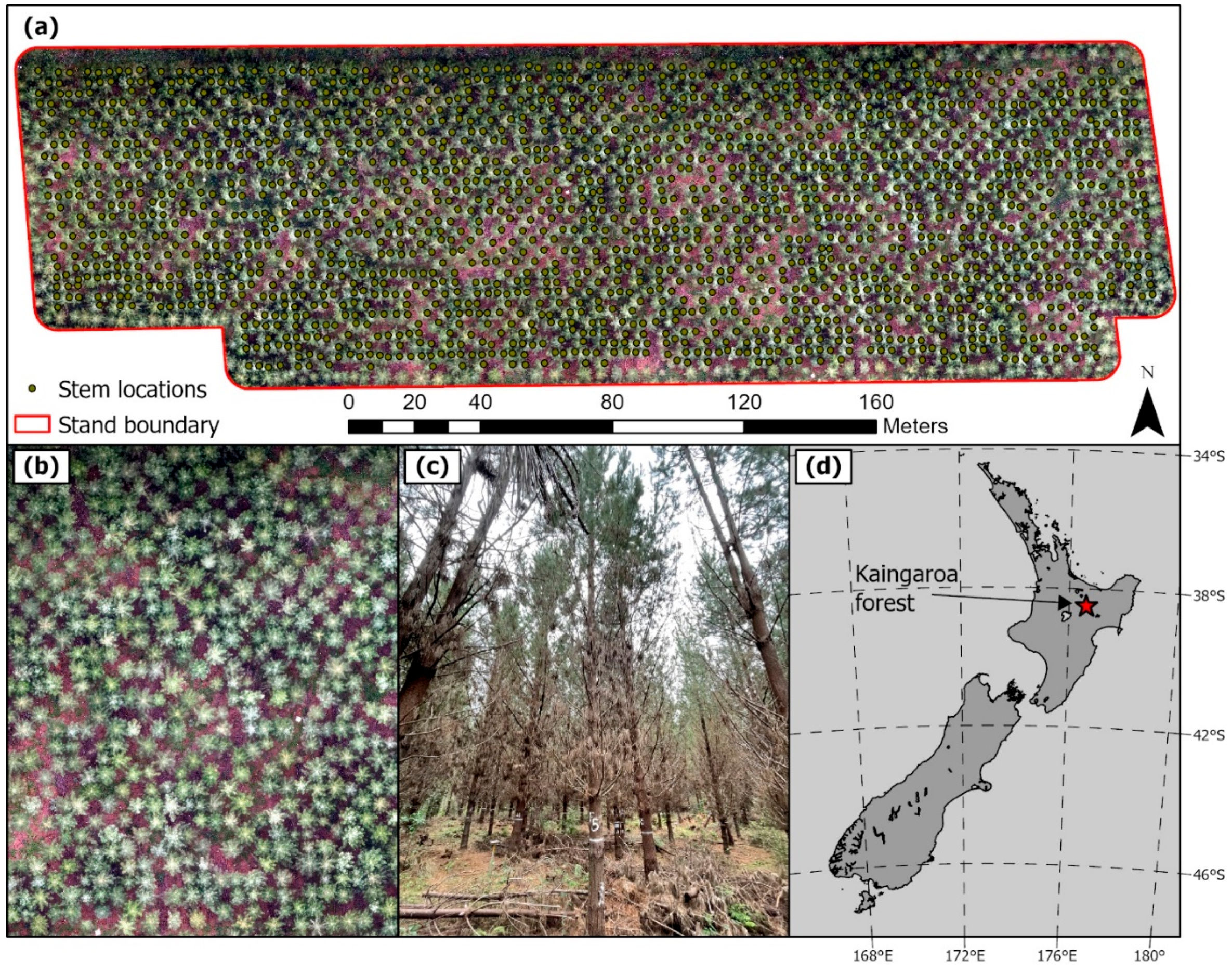
2.1. Study Site

This study was conducted in a 3-hectare trial within a plantation stand situated in Kaingaroa forest, which is located in the central region of New Zealand’s North Island (Figure 1). The site was established as a trial of elite clonal lines of radiata pine that was nine-year-old at the time of measurement. The trial is divided into 86 square grids, each covering an area of approximately 346 m2 that included 36 systematically planted trees, distributed across six rows with uniform square spacing at intervals of 3.1 m.
The initial stand density was 1040 stems/ha which was thinned at age 8 to a stand density of 456 stems/ha. All the remaining trees in the trial were also access pruned to a height of ~2 m to facilitate trial measurements. The terrain is predominantly flat, with some noticeable variations in slope along the northern and western boundaries, and has a moderately dense understory layer of shrubby blackberry (Rubus fruticosus L.).

2.2. Field Measurements

The field measurements were carried out from late February to early March 2023, over a period of two weeks. The recorded data included measurements of DBH and visual assessments of the condition of each tree. The DBH was measured using a diameter tape (accurate to 0.1 cm). The status of each tree was visually assessed according to standard forest inventory guidelines by an experienced forest inventory and mensuration technician. The standard forest inventory guidelines comprise more than 30 well-established categories that include various aspects of tree form, such as stem deformities and double/multi-leaders above DBH height. Summary statistics of tree attributes are presented in Table 1. Heights were not measured in the field as previous research has highlighted potential inaccuracies in field height measurement, caused by the difficulty in locating tree tops that can introduce bias [25]. As previous research has found minimal differences between field- and ULS-measured heights [26], ULS heights were used in this study.
To facilitate subsequent analysis, a stem map of the trial was created and validated on-site, and the spatial coordinates of individual trees were linked to their respective entries within the tree inventory.

2.3. LiDAR Data

2.3.1. Data Collection and Pre-Processing

Remote sensing data was acquired on 23 January 2023 using the DJI-Zenmuse L1 LiDAR and photogrammetry sensor. The sensor was mounted on a DJI Matrice 300 RTK platform (DJI, Shenzhen, China). The LiDAR acquisition was conducted at a flying speed of 3 m/s and an approximate altitude of 55 m above ground, using the Terrain Follow mode within the DJI Pilot 2 flight control software (version 1.1.5; DJI, Shenzhen, China). The vertical and horizontal beam divergences were recorded as 0.03° and 0.28°, respectively. The flight lines were systematically arranged in a gridded pattern, with a spacing of approximately 10 m between them. Flight spacing was planned to maintain an 85% forward and side overlap to facilitate improved point cloud colorization. The LiDAR system operated in the repetitive scan mode, with a LiDAR pulse frequency of 160 Hz. Up to three returns were recorded per laser pulse.
Point clouds were generated from the sensor’s native raw data format using the DJI Terra software (version 4.0.1; DJI, Shenzhen, China). The initial stage of raw point cloud processing involved the computation of point coordinates utilizing the base station coordinates. The point clouds were then georeferenced to the NZGD 2000 New Zealand Transverse Mercator coordinate system (EPSG 2193) and exported in laz format for further analysis. Technical specifications of the flight parameters and LiDAR data as well as the flight plan are detailed in Appendix A Table A1.
To gain insights into the spatial distribution of point density across the site, a density raster with a resolution of 1 m was generated. The resulting raster exhibited an average point density of 15,966 points/m2 and a standard deviation of 8500 points/m2. To eliminate small areas of exceptionally high point densities and ensure consistent point densities throughout the site, a homogenization process was applied to the point cloud. This homogenization aimed to achieve an initial maximum density of 24,450 points/m2, which is equivalent to the rounded mean density plus one standard deviation. The “sample_homogenize” function within the R software (version 4.3.3), lidR package [27] was implemented for this purpose [28]. This function employs an algorithm that generates a grid of a defined resolution and performs a random selection of points to be retained within each grid cell. The proportion of retained points within each grid cell is determined by assessing the local density in comparison to the desired density; in cases where the desired density exceeds the local density, the points remain unchanged.
The homogenized point cloud was then subjected to standard pre-processing steps, which included denoising, ground point classification, DTM generation, and ground normalization. These processing steps were executed using the LASTools software package (version 2.0.2) [29].

2.3.2. Individual Tree Segmentation

A canopy height model (CHM) with a resolution of 25 cm was generated by applying the pit-free algorithm developed by Khosravipour et al. (2014) [30] on the ground normalized point cloud. Subsequently, the CHM underwent smoothing through the implementation of a 3 × 3-pixel moving window. Individual tree peaks were then detected using a local maxima algorithm [31] with a fixed window size of 3 m, corresponding to the initial planting spacing of the site. Given the site’s predominantly homogeneous nature following the recent thinning, a minimum tree peak height of 6 m was used as the height threshold. The accuracy of the detected tree peaks was evaluated against the field-verified stem map of the study site, and any discrepancies were rectified. The adjusted tree peaks were then used as markers for individual tree crown delineation.
This delineation process was implemented on the smoothed CHM using the “mcws” function within the R software, ForestTools package [32], which employs a watershed algorithm for crown delineation. To ensure that the delineated crowns of individual trees did not merge into neighboring tree crowns and to prevent the inclusion of low vegetation within the identified tree crowns, the crown delineation was confined to the upper 75% of the CHM [33]. The polygons generated through the crown delineation process were subject to visual assessment to ensure their accuracy. Any inaccurately detected polygons were excluded from the subsequent analysis. Finally, the accurately delineated crown polygons were utilized to segment the ground-normalized LiDAR point cloud into discrete segments representing individual trees.

2.3.3. Metric Extraction

A comprehensive list of individual tree metrics, including metrics that describe various aspects of tree structure, was created based on the existing literature [34,35,36,37]. This list included metrics representing both the vertical and horizontal variations of individual tree foliage, as well as metrics that capture the two-dimensional (2D) and 3D structural characteristics of trees. These selected metrics were computed for each individual tree point cloud segment, using packages within the R software [28].
The derived metrics can be classified into three primary categories: point-based, area-based, and voxel-based. Point-based metrics, including standard height, intensity, and crown density, were calculated using the “stdmetric” function within the lidR package [27]. Gap fraction and leaf area density (LAD) metrics [38] were determined using the “gap_fraction_profile” function within the lidR package. Additionally, shape and scale parameters for a Weibull Probability Distribution (WPD) [36] were produced to approximate vertical canopy structure, using the fitdistrplus package [39]. When calculating the shape and scale, tree heights were normalized between 0 and 1 to focus exclusively on crown shape. A convex hull was fitted to each individual tree segment using the cxhull package [28] with the 2D area of the individual crown convex hull (cvx2D_area) and the 3D volume of the individual tree convex hull (cnx3D_vol) being estimated.
The point clouds were voxelized at a resolution of 25 cm using the VoxR package [40]. Subsequent to voxelization, the methodologies outlined by Lefsky et al. (1999) [37] were applied to derive vertical canopy structural metrics. The comprehensive list of metrics examined in this study is presented in Appendix A Table A2 and includes the following seven metric groups: (i) standard height, (ii) standard intensity, (iii) standard crown density, (iv) gap fraction and LAD, (v) vertical canopy structure, (vi) 2D and 3D convex hull measurements, and (vii) voxel-based canopy metrics.

2.3.4. Data Thinning

The advent of laser scanners such as DJI-L1 allows very high-density point clouds to be captured from relatively low-cost equipment. We hypothesize that the point density obtained from these scanners enables the computation of new metrics that enhance the spatial descriptions of forests. Similar densities can be achieved with other ULS sensors such as the VUX1 or VUX240, but this necessitates slower, lower, and denser flight patterns. In addition, sensors such as the DJIL1 provide forest owners with a cost-effective means of acquiring LiDAR data. When utilized operationally, there is likely to be interest in understanding how far point densities can be reduced, through flying faster, before predictive accuracy of key attributes is reduced. To address these concerns, the LiDAR data were subjected to a thinning process to produce a range of point densities which allowed the influence of point density on the accuracy of tree attribute modeling to be examined. The selected densities covered the range of densities achieved within forestry settings by various LiDAR platforms (i.e., aircraft, helicopter, and unmanned aerial vehicles (UAVs)), as well as the densities attainable through a combination of various flight parameter settings within consumer-grade sensors.
A thinning algorithm was applied to the homogenized point cloud, resulting in point clouds with target densities of 12,200, 6100, 3050, 1550, 750, 400, 200, 100, 50, 40, 30, 20, and 10 points/m2. The obtained decimated point clouds were utilized to generate 1 m resolution density rasters, which were later examined to ensure reasonable consistency of point density across the site.
It is important to note that reducing the point density through decimation might impact the number of ground points and consequently influence the accuracy of the DTM, potentially introducing cumulative errors into the ground normalized point cloud. To address this, a comparison was conducted between the DTMs derived from the decimated point clouds (referred to as native DTMs hereafter) and the DTM derived from the homogenized point cloud with a density of 24,450 points/m2 (referred to hereafter as the high-density DTM).
Following this, the decimated point clouds were subjected to identical preprocessing steps including denoising, ground classification, and DTM creation. The resulting pre-processed point clouds underwent ground normalization using two distinct methods: 1. using the native DTM and 2. employing the high-density DTM.
Subsequently, all 27 ground-normalized point clouds—14 normalized using the native DTM and 13 normalized using the high-density DTM—were passed through the individual tree segmentation and metric extraction processes described in Section 2.3.2 and Section 2.3.3. Figure 2 illustrates a segmented individual tree at different point densities.

2.4. Tree Structural Attribute Prediction

All modeling of tree structural attributes was undertaken within R [28]. All dead trees or those that had forked stems (also known as multi-leaders) were removed from the dataset. Following these exclusions, 1381 trees were available for model development. A test dataset, comprising 20% of the observations (276 trees) was randomly selected, withheld from model development, and used to test the accuracy of the models. The training dataset comprised the remaining 80% of observations (1105 trees).

2.4.1. Prediction of DBH

Predictions of DBH were made using partial least squares (PLS) and random forest (RF) which were implemented through the Caret (Classification And Regression Training) package that streamlines the creation and comparison of predictive models [41]. Model training was undertaken using a 10-fold cross-validation with five repeats. Under 10-fold cross-validation, the training dataset is randomly divided into ten equal-sized groups. During each round, the model is fitted to 90% of the data, with model validation undertaken on the remaining 10%. This process is repeated a further nine times until each of the ten groups has been used for validation. This entire process is then repeated five times and model evaluation statistics were averaged across all 50 subsampled (ten folds × five repeats) validation datasets. The final tuned models were then used to predict DBH on the withheld test dataset and the accuracy and bias of these predictions provided an independent assessment of model fit.
Partial least squares [42] is a parametric modeling method that uses uncorrelated components, which are linear combinations of the predictor variables, to model the dependent variable (for more details see [43,44]). In comparison to other parametric methods, PLS is useful when there are a large number of correlated variables in the dataset. The number of components is a tunable hyperparameter within PLS. Random forest is a widely used non-parametric tree-based method that is able to account for non-linear relationships and is robust to collinearity between predictor variables [45,46]. The RF algorithm was implemented through the ranger package [47], and tunable hyperparameters included the split rule, number of trees, minimum node size, and the number of predictors that are randomly selected as candidates for splitting at each node. Models were developed across the range of point densities using both PLS and RF for datasets that had DTMs created using the native and highest pulse densities. Thus, there were 54 models in total, which comprised 27 pulse densities (14 point densities with the native DTM—including the highest point density of 24,450 points/m2—and 13 with the high-density DTM) × two algorithms. These 54 models used the entire suite of LiDAR metrics displayed in Appendix A Table A2. The most important variables among these LiDAR metrics were identified using the varImp function in the Caret package.
Among the seven variable types, the groups that had the strongest influence on model performance were identified by constructing models in turn using metrics from each of these seven groups. These models were fitted to each of the 14 point densities that were constructed using the native DTM dataset. Partial least squares were used for variable types with five or more predictive variables and linear regression for the two groups that included only two predictive variables (area-based metrics and vertical canopy structure). As there was high collinearity between the two variables for the area-based metrics (R2 > 0.8) code was written to select, for each point density, the variable that was most strongly related to DBH. In contrast, collinearity was relatively low for the vertical canopy structure metrics (R2 < 0.5), so both variables were included in each of the 14 models. For both variable types, polynomial terms were included in the linear models when they were significant and improved model accuracy.

2.4.2. Prediction of Volume

The accuracy of volume predictions was assessed against a reference volume across the 14 different point densities. Following [48], tree volume was computed from DBH and height using the following equation,
V = h × ba × (a × (h − 1.4)b + c),
where h is tree height, ba is basal area and parameters a, b, and c have values of, respectively, 0.860, 0.972, and 0.340. This function was developed using data from radiata pine stands located in the same region as the study site [48]. Using Equation (1), the reference volume was computed from the field-measured DBH and LiDAR point-based zmax, which is defined as the maximum height of the unthinned point cloud.
For each of the 14 point densities, normalized using the native DTM, V was predicted from zmax, extracted from the individual tree point clouds, and model predictions of tree DBH that were made using PLS. Using the test dataset, predicted values of volume were regressed against the reference volume for each point density, and model statistics were extracted to evaluate accuracy.

2.5. Accuracy Assessment

Detected tree peaks were tested against the field-verified stem map to assess the accuracy of the tree peak detection. Common accuracy assessment statistics were calculated using the following formulae:
P r e c i s i o n = T P T P + F P
R e c a l l = T P T P + F N
F 1   score   = 2 × R e c a l l × P r e c i s i o n R e c a l l + P r e c i s i o n
where T P , F P , and F N are, respectively, true positive (a prediction that correctly indicates the presence of a tree), false positive (a prediction that incorrectly indicates the presence of a tree), and false negative (a prediction that incorrectly indicates the absence of a tree) predictions. Precision measures the proportion of correct positive predictions, while recall identifies the fraction of true positives accurately identified. As the harmonic mean of precision and recall, the F1 score can be categorized as representing poor (0.5–0.7), acceptable (0.7–0.8), excellent (0.8–0.9), and outstanding (>0.9) levels of detection.
The accuracy of the decimated CHM and DTM and models that predicted DBH and volume was assessed using the root mean square error (RMSE), mean bias error (MBE), and the coefficient of determination (R2) which were calculated as follows:
R M S E = i = 1 n ( y ^ i y i ) 2 n
M B E = 1 n i = 1 n y i y ^ i
R 2 = i ( y ^ i y ¯ ) 2 i ( y i y ¯ ) 2
where y i , y ^ i , y ¯ , and n , respectively, represent reference or measured values, predicted values, an average of the reference or measured values, and the sample size.

3. Results

3.1. Accuracy of Individual Tree Segmentation

An F1 score exceeding 0.96 was observed across all tested point densities and increased from 0.96 at point densities < 100 points/m2 to 0.97 at all point densities above this value, for both types of DTM (Appendix A Table A3). While recall marginally increased from 0.95–0.96 at 10 points/m2 to 0.98 at the highest point densities, precision slightly declined with increasing pulse density from ca. 0.98 to 0.96 across this range, for both DTMs. This indicated that at low point densities there were slightly more false negatives than false positives, while the reverse was true at high point densities. The proportion of accurately delineated crowns increased with point density from 96% at 10 points/m2 to 0.98 at 20 points/m2 and was 0.99 for point densities of ≥ 30 points/m2 for both DTM types.

3.2. DTM and CHM Assessment
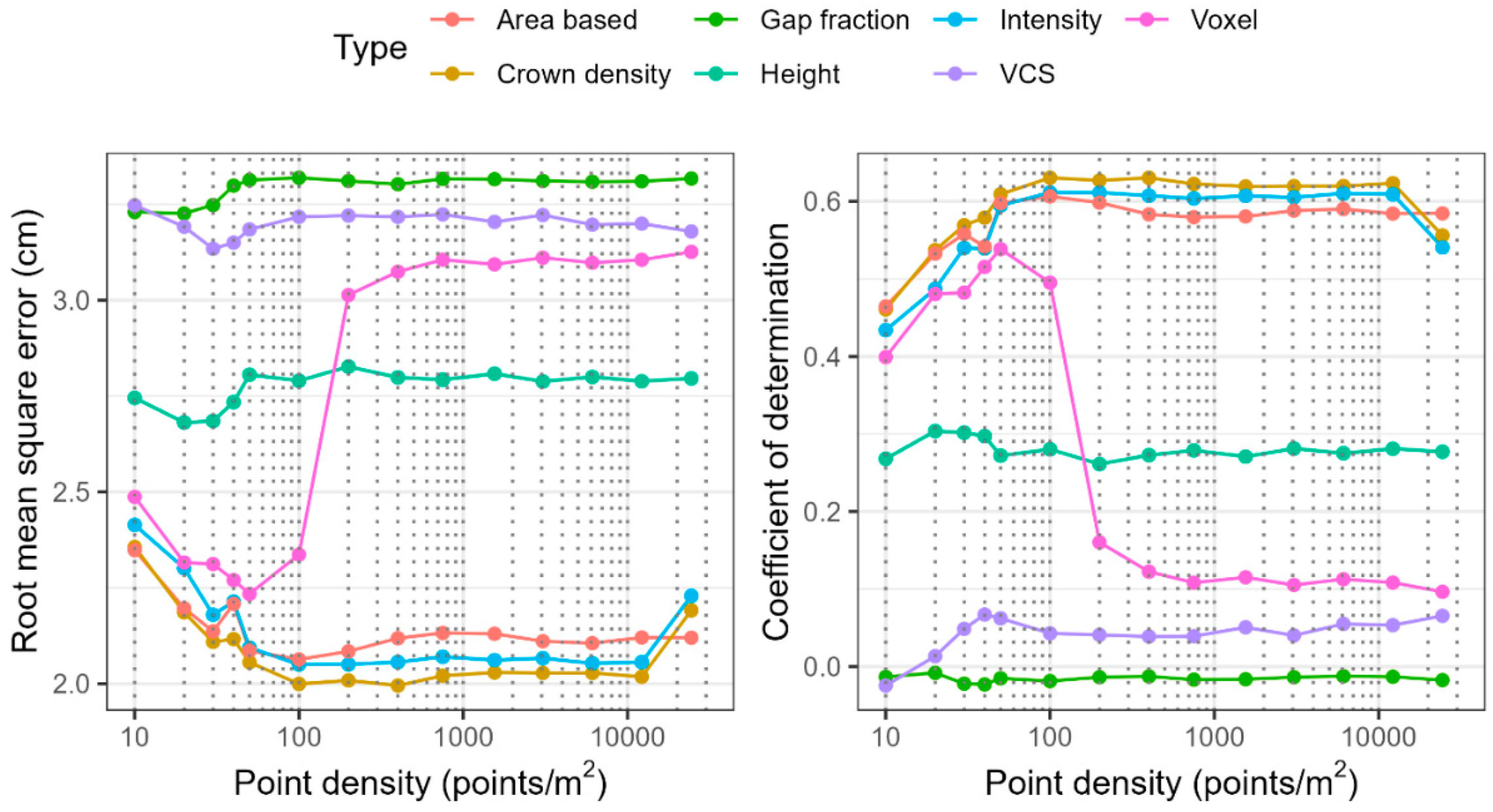
There was little difference between the native DTMs obtained from decimated point clouds and the highest density point cloud, with the RMSE ranging from 0.02 m to 0.11 m (Table 2). Compared to the high density DTM, the height of the ground was slightly underestimated by the thinned datasets with MBE increasing from 0–0.06 m as the point density declined (Table 2). Compared to the unthinned CHM the thinned CHMs showed increases in height as the point cloud density diminished, with MBE ranging from −0.01 m at 12,200 points/m2 to −3.12 m at 10 points/m2. This systematic bias was accompanied by an increase in the RMSE with reductions in point density (Table 2).

3.3. DBH Prediction

Models of DBH using PLS had higher accuracy than those using RF at all point densities, for both the high and native DTM categories (Figure 3). Differences in accuracy between the two modeling methods generally increased with point density. For each algorithm, little variation in accuracy was noted between the two types of DTM across the point density range. For all four combinations of modeling methods and DTM types, model accuracy was generally highest at 12,200 points/m2.
As data was thinned accuracy remained relatively stable until point densities of ca. 750 points/m2 were reached, below which there was a gradual decline in accuracy to ca. 50 points/m2 after which point accuracy declined far more rapidly. Given that PLS was the more accurate algorithm and the use of the high-density DTM did not provide any gain in accuracy, further analyses use PLS with the native DTM.
Focusing on the PLS method, using the native DTM, the accuracy at 12,200 points/m2 (RMSE = 1.624 cm and R2 = 0.756) was relatively similar for thinned datasets to a point density of 400 points/m2 (RMSE = 1.635 cm; R2 = 0.752) (Figure 3). As data was thinned, below this point, accuracy declined slowly to 50 points/m2 (RMSE = 1.693 cm; R2 = 0.735) and then more rapidly to 10 points/m2 (RMSE = 1.983 cm; R2 = 0.618). Across these 14 models, the most important variable was cnx3D_vol (in 9 models), followed by imean (in two models) then isd, imean, and zmax, which were all most important in one model (see Appendix A Table A2 for metric description).
Further insight into the most important variable types is given in Figure 4 which shows changes in model accuracy in response to point density by variable type. The area-based, crown density, and intensity metrics were the metric classes that produced the most accurate models, and all showed similar changes in accuracy with point density. The accuracy of models created using thinned point clouds with metrics from these three classes was relatively invariant down to a point density of 100 points/m2, below which accuracies showed a marked decline. Generally, models created using crown density metrics were more accurate than those using intensity metrics which in turn slightly exceeded the accuracy of models using area-based metrics. However, there was an interchange in this ranking between these groups particularly at lower and very high point densities. Models that used area-based metrics were more accurate than those using intensity metrics at point densities ≤ 50 points/m2 and the variable selection process, chose cnx3D_vol as the most important variable for all 14 models created using area-based metrics.
Models created using voxelized metrics increased in accuracy to a point density of 50 points/m2, above which there were significant reductions in accuracy, that stabilized at ca. 400 points/m2 (Figure 4). This pattern broadly reflected changes in models created using the most important variable in this class (filled canopy) where accuracy increased sharply from 10 to between 20–100 points/m2 before declining with further increases in point density. Models of DBH created using height metrics had an intermediate accuracy that was relatively invariant to point density with RMSE and R2, respectively, ranging across point densities by 2.68–2.83 cm and 0.261–0.304. Models that used either vertical crown structure metrics or gap fraction metrics were relatively inaccurate across the range of point densities (Figure 4).

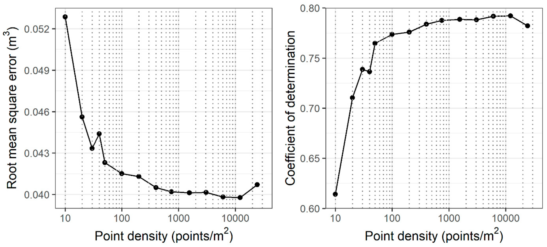
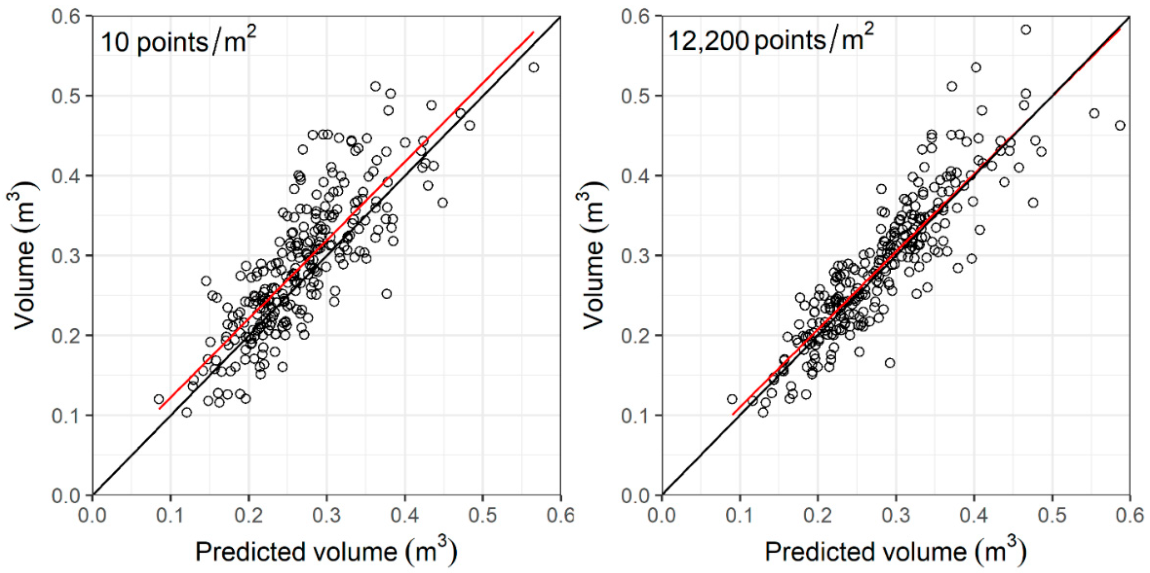
3.4. Volume Prediction

Using Equation (1), PLS predictions of DBH were used in combination with the LiDAR metric zmax, derived from the individual tree point clouds, to predict tree volume for the 14 point densities created using the native DTMs. These predicted values were then plotted against a reference volume derived from actual DBH and the zmax obtained from the unthinned point cloud (point density = 24,450 points/m2). The accuracy of these volume predictions, obtained from the test dataset, is shown in Figure 5. At the maximum thinned point density of 12,200 points/m2, volume was predicted with high accuracy, with RMSE of 0.0418 m3 and R2 of 0.792. The accuracy of these predictions was relatively invariant to reductions in point density until 750 points/m2 (RMSE = 0.0402 m3; R2 = 0.788), below which there was a gradual reduction in accuracy to 50 points/m2 (RMSE = 0.0423 m3; R2 = 0.765) and then a sharp drop to 10 points/m2 (RMSE = 0.0529 m3; R2 = 0.614).
Predictions using the most accurate (12,200 points/m2) and least accurate (10 points/m2) point densities are shown in Figure 6. At the lower point density, the reference volume was slightly underpredicted across the range in volume. In contrast, the plot of predicted against reference volume for the higher point density showed little apparent bias.

4. Discussion

4.1. Robustness of Individual Tree Segmentation, DTM and CHM across Varying Point Densities

The accurate detection and segmentation of trees play a crucial role in various forestry applications, including tree counting, biomass estimation, and forest health assessment. The detection accuracy depends on many factors, including tree species, forest complexity, point density, algorithm selection, and data quality [31,49,50,51,52]. One of the most important factors for tree-level characterization is the density and accuracy of point clouds. The advent of commercial-grade solid-state LiDAR units such as the L1 makes the acquisition of ultra-high-density forest point clouds practical and cost-effective.
The use of the LiDAR L1 data in combination with a local maxima-based technique provided a very accurate means of detecting individual tree peaks. Detection accuracy was outstanding with the F1 score varying from 0.96 to 0.99 across the range of point densities. This very high classification accuracy was most likely enhanced by the recent thinning of the stand coupled with the utilization of key structural features of the stand. As the stand had been recently thinned and had minimal canopy overlap, there were few hard-to-detect suppressed trees beneath the larger canopies. Through using the initial planting spacing as the window size for the local maxima algorithm we were able to prevent multiple peak detection within a single crown. The use of a high minimum height threshold of 6 m further restricted excessive false positive detections.
The CHM resolution can have a strong impact on local maxima detection [51,53]. Extremely low resolutions may lead to a smoothing effect on individual canopy heights, resulting in tree peaks being missed, while extremely high resolutions can lead to multiple peak detections on an individual tree from fine details such as large branches [54]. In this study, the optimal overall segmentation accuracy was achieved with a CHM resolution of 25 cm, although customization may be needed for other forest types and plantation settings. Previous literature indicates that unsupervised CHM-based segmentation methods, such as the watershed algorithm, are prone to over-segmentation [16,51]. This research used detected tree peaks as seed points for segmentation initiation, effectively demonstrating how a supervised watershed segmentation method can address challenges related to over-segmentation and achieve higher accuracy.
Point clouds contain a collection of 3D data points that intricately describe the surface of various objects within a forest environment, including tree crowns, other vegetation, and terrain. Therefore, the accuracy and reliability of forest surfaces such as the DTM and CHM are inherently linked to the abundance of data points captured within the point cloud [50,51]. The created native DTMs were relatively accurate down to several low point densities and exhibited little disparity with the high-density DTM due to the relative flatness of the site. However, underestimation of DTM values can occur due to ground elevation interpolation between points in complex terrain and where laser penetration is hindered by dense understory not adequately captured in low-density point clouds [24,55].
In contrast to the DTMs, point density had a stronger impact on the CHMs. Increasing point cloud density improved CHM detail and the accuracy of the crown delineation. This enhancement was mainly attributed to the increased availability of data points, which allows for a more accurate depiction of fine details in canopy structures, including the extended branches [56,57,58]. In contrast, CHMs from low-density point clouds overestimated values due to limitations in representing vegetation height details [57]. In cases of insufficient point density, models inaccurately portray complex canopy features, leading to imprecise crown delineations [58]. Our results support this finding as we also observed crown delineation imprecision increasing at densities below 100 points/m2.

4.2. Accuracy and Sensitivity of Forest Structural Attribute Estimation

The predictions of DBH and volume shown here were relatively accurate. Previous research has developed similar models in tropical forests [22], mixed coniferous forests [23], and broadleaf plantations [24], utilizing both ALS [22,23] and ULS [24] data. Comparable prediction accuracies have previously been observed in several studies that examined the effectiveness of various modeling algorithms for predicting forest structural attributes in different forest settings. These studies examined a range of techniques, including PLS, RF, linear regression model (LM), linear model with ridge regularization (LMR), support vector regression (SVR), k-Nearest Neighbors (k-NN), and artificial neural network (ANN). Our predictions of model accuracy at higher pulse densities using PLS were within this previously reported range where R2 values varied from 0.68 to 0.89 for estimations of DBH [24,49,54,59] and 0.70 to 0.93 [24,54,60] for stem volume predictions. [24,54,60]
This study showed that PLS consistently outperformed RF models in terms of accuracy, irrespective of point density, and DTM type. This finding suggests that PLS is more effective in capturing the relationships between LiDAR-derived metrics and individual tree structural attributes, thus leading to improved model predictions. Previous research has reported that PLS had the highest prediction accuracy (R2 = 0.97) compared to RF and k-NN for Lorey’s mean height, whereas k-NN outperformed PLS in predicting volume [24]. Interestingly, the disparity in accuracy between PLS and RF models appeared to increase as point density increased. This trend could be attributed to the ability of PLS to more effectively handle multicollinearity among variables [44], which becomes more pronounced at higher point densities. For both modeling approaches, model predictions of DBH had a very similar accuracy between the two DTM types. In contrast to previous studies [55,61,62], this finding suggests that DTM quality may not have a major influence on attribute prediction particularly on sites with relatively flat terrain.
Using the PLS method model accuracy was generally stable down to 400 points/m2 after which there were slight reductions in accuracy to 50 points/m2 and then more marked reductions to 10 points/m2. The threshold point density of 400 points/m2 may represent a balance wherein sufficient information is available to support accurate predictions without introducing unnecessary noise. Although accuracy did not decline above this threshold of 400 points/m2 the results suggest that higher point densities do not contribute additional useful information to the models.
The key predictive variables that were identified offer valuable insights for making informed decisions when selecting important metrics for DBH and volume modeling. The metric cnx3D_vol, which was the most frequently used variable, and accounted for > 50% of the variance in almost all models, had a sound basis for inclusion as it represents the 3D volume of the convex hull fitted around the individual tree segment. Previous studies have consistently reported that crown metrics, including crown projection area, crown surface area, and crown volume, are an important class of variable for DBH and volume predictions [52,63,64].
Voxel metrics were important predictors of DBH at point densities ranging from 20–100 points/m2 but the strength of these correlations diminished at point densities lower or higher than this range. At densities of 10 points/m2, the points were likely to be too sparsely distributed to allow the development of meaningful metrics. In contrast, at higher point densities, the reduced predictive power most likely resulted from data saturation and redundancy.
A number of studies have used ULS to predict tree diameter or volume directly from point cloud data using methods such as quantitative structure modeling (QSM) that reconstruct the surface geometry of the stem [65,66,67]. However, these methods are often used under ideal conditions and recent research shows QSM predicts DBH with low accuracy under standard forestry conditions [65]. Under these circumstances, it was necessary to fuse ULS data with LiDAR collected from ground-based sensors to estimate DBH with high precision [65]. However, we have tested LiDAR from a mobile laser scanner within a range of unpruned radiata pine stands and found that the dense needle cover makes it impossible to reconstruct the stem in unpruned stands [68] which constitute the majority of New Zealand plantation forests [3]. In contrast, the models employed here, use canopy metrics, that can be more robustly characterized from ULS. Although the methods used here do not measure DBH and volume as directly as QSM, the developed models were relatively accurate and show significant potential for commercial deployment.
Further research should focus on exploring the generality of the approach used in this study. The method should be extended to different forest types, species, and stand conditions, under a range of environmental conditions to assess the robustness of the method and consumer-grade UAV data. Conducting temporal studies within the same stand or testing consumer-grade LiDAR sensors within stands of differing age classes and silvicultural treatments will also provide insight into the method generality. The approach used here may not suit all stands and site conditions and it is important to identify factors that limit the application of the method. The assembly and analysis of these data will provide a means of assessing the stand conditions that most suit the approach and could be distilled into a set of guidelines outlining conditions under which the method can be used.

5. Conclusions

This study presented a comprehensive analysis of the potential of a consumer-grade LiDAR sensor for key inventory applications that included individual tree segmentation, and the prediction of DBH and stem volume. The accuracy of these products was evaluated across varying point densities using DTMs that were created at native and the highest point density (24,450 points/m2). The local maxima-based method used for tree peak detection accurately detected individual trees, consistently yielding outstanding F1 scores that exceeded 0.96 at all examined densities. Models of DBH created using PLS had a consistently higher accuracy than those that used RF, but there was little variation in accuracy between the models created using different DTMs. Using data from the native DTMs, DBH estimation using PLS had the lowest RMSE of 1.624 cm (R2 of 0.756) at a point density of 12,200 points/m2. Predictions of stem volume had an RMSE of 0.0418 m3 (R2 of 0.792) at the same point density. The accuracy of these predictions for DBH and volume were stable in decimated point clouds to 400 points/m2 after which there were small reductions in precision to 50 points/m2 and then more marked reductions in accuracy to 10 points/m2. The recurring prominence of 3D crown volume metrics within models created using a range of point densities demonstrated the pivotal role of crown metrics in predicting DBH and volume at the individual tree level. These findings demonstrate the potential of consumer-grade ULS sensors for the rapid and frequent assessment of plantation forests and these sensors could provide forest managers with an affordable method to obtain tree-level inventory data. Further research should test the accuracy of the methodology described here across a broader range of species, stand, and site conditions, in order to gain an improved understanding of the generality of the approach.

Author Contributions

Conceptualization, S.J. and G.D.P.; methodology, M.S.W., S.J. and R.J.L.H.; validation, M.S.W. and S.J.; formal analysis, M.S.W. and S.J.; investigation, M.S.W. and S.J.; resources, R.J.L.H. and P.D.M.; data curation, R.J.L.H., P.D.M., D.C., B.S.C.S. and H.J.C.E.; writing—original draft preparation, S.J. and M.S.W.; writing—review and editing, R.J.L.H., G.D.P., P.D.M., D.C., B.S.C.S. and H.J.C.E.; supervision, M.S.W. and G.D.P.; funding acquisition, M.S.W. and G.D.P.; Visualization, B.S.C.S. All authors have read and agreed to the published version of the manuscript.

Funding

This research was funded by the Ministry of Business, Innovation and Employment (MBIE), programme entitled “Seeing the forest for the trees: transforming tree phenotyping for future forests” (programme grant number C04X2101).

Data Availability Statement

The data used in this study cannot be made publicly available due to privacy restrictions imposed by the forest owners and managers.

Acknowledgments

The authors extend their gratitude to Nicholas Coops and the members of his laboratory, particularly Liam Irwin and Sarah Smith-Tripp, for their invaluable insights and suggestions on the processing of DJI L1 data. We also would like to acknowledge Lukas Winiwarter for his invaluable insights on point decimation. Additionally, the authors would like to thank Timberlands Ltd. and Radiata Pine Breeding Company for access to the site and express their appreciation to Interpine Innovation for their assistance in the field inventory. The authors also would like to acknowledge Warren Yorston, and Samuel Wong for their contributions to the on-site validation of the stem map, and John Henry for assisting with site set up. Also, we extend our gratitude to Grant Evans, Joane Elleouet, and Russell Main from Scion for their feedback on the manuscript before its submission. We are grateful to the anonymous reviewers for comments that greatly improved the manuscript.

Conflicts of Interest

The authors declare no conflicts of interest.

Appendix A

Table A1. Technical specifications of the flight parameters and LiDAR data characteristics.
ParameterSpecification
SensorDJI-Zenmuse L1 LiDAR and Photogrammetry sensor
Capture date23 January 2023
Flying speed (m/s)3
Flying height above ground (m)55
Distance between flight lines (m)10
Number of scan layers2 (Gridded: Perpendicular to each other)
Scan modeRepetitive scanning
LiDAR strike frequency (Hz)160
Laser wavelength (nm)905
Field of view (°)70.4 (horizontal) × 4.5 (vertical)
Beam divergence (°)0.03 (horizontal) × 0.28 (vertical)
Number of returns3
Average (standard deviation) density of resulting point cloud (points/m2)15,966 (8500)
Table A2. Description of LiDAR metrics used in this study. NA: Not applicable.
ClassAbbreviationDescriptionR Package
Point-based metrics
1. Standard height metricszmaxMaximum height above groundlidR
zmeanMean height above ground
zsdStandard deviation of height distribution
zcvCoefficient of variation of height distribution
zskewSkewness of height distribution
zkurtKurtosis of height distribution
zentropyEntropy of height distribution
zq(X), where X is a percentile, (e.g., zq95)Percentile heights (5th, 10th, 15th, 20th, 25th, 30th, 35th, 40th, 45th, 50th, 55th, 60th, 65th, 70th, 75th, 80th, 85th, 90th, and 95th)
2. Standard intensity metricsitotSum of the intensity of returnslidR
imaxMaximum intensity of returns
imeanMean intensity of returns
isdStandard deviation of intensity distribution
icvCoefficient of variation of intensity distribution
iskewSkewness of intensity distribution
ikurtKurtosis of intensity distribution
ipgroundIntensity of ground returns
ipcumzq(X),
e.g., ipcumzq90
Percentage of intensity returned below the Xth height percentile
3. Standard crown density metricszpcum(X), e.g., zpcum9,Cumulative percentage of return in the Xth layerlidR
pgroundPercentage of returns classified as “ground”
pzabovezmeanPercentage of returns above the mean height of each tree
pzabove2Percentage of returns above 2 m height
p1st, p2nd, p3rdPercentage of returns (first return–third return)
nTotal number of points
4. Gap fraction and LAD metricsgfp_mMean of gap fraction profile (layer thickness: 1 m)lidR
gfp_sdStandard deviation of gap fraction profile
gfp_IQRInterquartile range of gap fraction profile
lad_mMean of leaf area density
lad_sdStandard deviation of leaf area density
5. Vertical canopy structural metricswpd_scaleWeibull probability distribution fitted to foliage profile: scale parameter αfitdistrplus
wpd_shapeWeibull probability distribution fitted to foliage profile: shape parameter β
Area-based metrics
6. 2D and 3D convex hull metricscvx2D_area2D area of individual crown convex hullcxhull
cnx3D_vol3D volume of the individual tree convex hull
Voxel-based metrics (25 cm voxel res)
7. Voxel-based vertical canopy structural metricsfilled_canopyFilled canopy volume percentage: Proportion of total number of voxels containing pointsNA
open_gapOpen gap volume percentage: Proportion of voxels containing no points above the canopy
closed_gapClosed gap volume percentage: Proportion of voxels containing no points below the canopy
euphoticEuphotic volume percentage: Proportion of voxels in the uppermost 65% of cells that contain points of a column
oligophoticOligophotic volume percentage: Proportion of voxels in the lower 35% of cells that contain points in a column
Table A3. Assessment of individual tree detection and segmentation results across varying point densities. NA: Not applicable.
Maximum Density of Source Point Cloud (points/m2)Point Cloud Ground Normalized Using the Highest Density DTMPoint Cloud Ground Normalized Using the Native DTM
Tree Peak Detection AccuracyCrown Delineation AccuracyTree Peak Detection AccuracyCrown Delineation Accuracy
PrecisionRecallF1Proportion of Accurately Delineated CrownsPrecisionRecallF1Proportion of Accurately Delineated Crowns
100.980.950.960.960.970.950.960.96
200.980.950.960.980.980.950.960.98
300.980.950.960.990.980.950.960.99
400.980.950.960.990.980.950.960.99
500.970.960.960.990.970.960.960.99
1000.970.970.970.990.970.960.960.99
2000.970.970.970.990.970.970.970.99
4000.970.980.970.990.970.980.970.99
7500.960.980.970.990.960.980.970.99
15500.960.980.970.990.960.980.970.99
30500.960.980.970.990.960.980.970.99
61000.960.980.970.990.960.980.970.99
12,2000.960.980.970.990.960.980.970.99
24,450NANANANA0.960.980.970.99

References

  1. FAO. Global Forest Resources Assessment 2020—Key Findings; FAO: Rome, Italy, 2020; p. 5. [Google Scholar] [CrossRef]
  2. Bukoski, J.J.; Cook-Patton, S.C.; Melikov, C.; Ban, H.; Chen, J.L.; Goldman, E.D.; Harris, N.L.; Potts, M.D. Rates and drivers of aboveground carbon accumulation in global monoculture plantation forests. Nat. Commun. 2022, 13, 4206. [Google Scholar] [CrossRef]
  3. NZFOA. New Zealand Forestry Industry, Facts and Figures 2021/2022; New Zealand Plantation Forest Industry: Wellington, New Zealand, 2022. [Google Scholar]
  4. Koutika, L.; Matondo, R.; Mabiala-Ngoma, A.; Tchichelle, V.S.; Toto, M.; Madzoumbou, J.; Akana, J.A.; Gomat, H.Y.; Mankessi, F.; Mbou, A.T.; et al. Sustaining Forest Plantations for the United Nations’ 2030 Agenda for Sustainable Development. Sustainability 2022, 14, 4624. [Google Scholar] [CrossRef]
  5. Vidal, C.; Alberdi, I.; Redmond, J.; Vestman, M.; Lanz, A.; Schadauer, K. The role of European National Forest Inventories for international forestry reporting. Ann. For. Sci. 2016, 73, 793–806. [Google Scholar] [CrossRef]
  6. Roise, J.P.; Cubbage, F.W.; Abt, R.C.; Siry, J.P. Regulation of Timber Yield for Sustainable Management of Industrial Forest Plantations—Theory and Practice. In Sustainable Forest Management; Springer: Dordrecht, The Netherlands, 2000; pp. 217–255. [Google Scholar]
  7. Maltamo, M. Estimation of timber volume and stem density based on scanning laser altimetry and expected tree size distribution functions. Remote Sens. Environ. 2004, 90, 319–330. [Google Scholar] [CrossRef]
  8. Zhao, D.; Kane, M.; Borders, B.E. Growth responses to planting density and management intensity in loblolly pine plantations in the southeastern USA Lower Coastal Plain. Ann. For. Sci. 2011, 68, 625–635. [Google Scholar] [CrossRef]
  9. Kanninen, M.; Pérez, D.; Montero, M.; Víquez, E. Intensity and timing of the first thinning of Tectona grandis plantations in Costa Rica: Results of a thinning trial. For. Ecol. Manag. 2004, 203, 89–99. [Google Scholar] [CrossRef]
  10. Hébert, F.; Krause, C.; Plourde, P.-Y.; Achim, A.; Prégent, G.; Ménétrier, J. Effect of Tree Spacing on Tree Level Volume Growth, Morphology, and Wood Properties in a 25-Year-Old Pinus banksiana Plantation in the Boreal Forest of Quebec. Forests 2016, 7, 276. [Google Scholar] [CrossRef]
  11. Zhu, Z.; Kleinn, C.; Nölke, N. Assessing tree crown volume—A review. For. Int. J. For. Res. 2021, 94, 18–35. [Google Scholar] [CrossRef]
  12. Zhen, Z.; Quackenbush, L.; Zhang, L. Trends in Automatic Individual Tree Crown Detection and Delineation—Evolution of LiDAR Data. Remote Sens. 2016, 8, 333. [Google Scholar] [CrossRef]
  13. Brūmelis, G.; Dauškane, I.; Elferts, D.; Strode, L.; Krama, T.; Krams, I. Estimates of Tree Canopy Closure and Basal Area as Proxies for Tree Crown Volume at a Stand Scale. Forests 2020, 11, 1180. [Google Scholar] [CrossRef]
  14. White, J.C.; Coops, N.C.; Wulder, M.A.; Vastaranta, M.; Hilker, T.; Tompalski, P. Remote Sensing Technologies for Enhancing Forest Inventories: A Review. Can. J. Remote Sens. 2016, 42, 619–641. [Google Scholar] [CrossRef]
  15. Torresan, C.; Berton, A.; Carotenuto, F.; Di Gennaro, S.F.; Gioli, B.; Matese, A.; Miglietta, F.; Vagnoli, C.; Zaldei, A.; Wallace, L. Forestry applications of UAVs in Europe: A review. Int. J. Remote Sens. 2016, 38, 2427–2447. [Google Scholar] [CrossRef]
  16. Puliti, S.; Ene, L.T.; Gobakken, T.; Næsset, E. Use of partial-coverage UAV data in sampling for large scale forest inventories. Remote Sens. Environ. 2017, 194, 115–126. [Google Scholar] [CrossRef]
  17. Štroner, M.; Urban, R.; Línková, L. A New Method for UAV Lidar Precision Testing Used for the Evaluation of an Affordable DJI ZENMUSE L1 Scanner. Remote Sens. 2021, 13, 4811. [Google Scholar] [CrossRef]
  18. Watt, M.S.; Meredith, A.; Watt, P.; Gunn, A. The influence of LiDAR pulse density on the precision of inventory metrics in young unthinned Douglas-fir stands during initial and subsequent LiDAR acquisitions. N. Z. J. For. Sci. 2014, 44, 18. [Google Scholar] [CrossRef]
  19. Pearse, G.D.; Watt, M.S.; Dash, J.P.; Stone, C.; Caccamo, G. Comparison of models describing forest inventory attributes using standard and voxel-based lidar predictors across a range of pulse densities. Int. J. Appl. Earth Obs. Geoinf. 2019, 78, 341–351. [Google Scholar] [CrossRef]
  20. Treitz, P.; Lim, K.; Woods, M.; Pitt, D.; Nesbitt, D.; Etheridge, D. LiDAR Sampling Density for Forest Resource Inventories in Ontario, Canada. Remote Sens. 2012, 4, 830–848. [Google Scholar] [CrossRef]
  21. Hansen, E.; Gobakken, T.; Næsset, E. Effects of Pulse Density on Digital Terrain Models and Canopy Metrics Using Airborne Laser Scanning in a Tropical Rainforest. Remote Sens. 2015, 7, 8453–8468. [Google Scholar] [CrossRef]
  22. Manuri, S.; Andersen, H.-E.; McGaughey, R.J.; Brack, C. Assessing the influence of return density on estimation of lidar-based aboveground biomass in tropical peat swamp forests of Kalimantan, Indonesia. Int. J. Appl. Earth Obs. Geoinf. 2017, 56, 24–35. [Google Scholar] [CrossRef]
  23. Jakubowski, M.K.; Guo, Q.; Kelly, M. Tradeoffs between lidar pulse density and forest measurement accuracy. Remote Sens. Environ. 2013, 130, 245–253. [Google Scholar] [CrossRef]
  24. Liu, K.; Shen, X.; Cao, L.; Wang, G.; Cao, F. Estimating forest structural attributes using UAV-LiDAR data in Ginkgo plantations. ISPRS J. Photogramm. Remote Sens. 2018, 146, 465–482. [Google Scholar] [CrossRef]
  25. Wang, Y.; Lehtomäki, M.; Liang, X.; Pyörälä, J.; Kukko, A.; Jaakkola, A.; Liu, J.; Feng, Z.; Chen, R.; Hyyppä, J. Is field-measured tree height as reliable as believed—A comparison study of tree height estimates from field measurement, airborne laser scanning and terrestrial laser scanning in a boreal forest. ISPRS J. Photogramm. Remote Sens. 2019, 147, 132–145. [Google Scholar] [CrossRef]
  26. Hartley, R.J.L.; Leonardo, E.M.; Massam, P.; Watt, M.S.; Estarija, H.J.; Wright, L.; Melia, N.; Pearse, G.D. An Assessment of High-Density UAV Point Clouds for the Measurement of Young Forestry Trials. Remote Sens. 2020, 12, 4039. [Google Scholar] [CrossRef]
  27. Roussel, J.-R.; Auty, D.; Coops, N.C.; Tompalski, P.; Goodbody, T.R.H.; Meador, A.S.; Bourdon, J.-F.; de Boissieu, F.; Achim, A. lidR: An R package for analysis of Airborne Laser Scanning (ALS) data. Remote Sens. Environ. 2020, 251, 112061. [Google Scholar] [CrossRef]
  28. R Core Team. R: A Language and Environment for Statistical Computing; R Foundation for Statistical Computing: Vienna, Austria, 2023. [Google Scholar]
  29. Isenburg, M. LAStools—Efficient LiDAR Processing Software, Version 2.0.2; Rapidlasso GmbH: Gilching, Germany, 2019. [Google Scholar]
  30. Khosravipour, A.; Skidmore, A.K.; Isenburg, M.; Wang, T.; Hussin, Y.A. Generating pit—Free canopy height models from airborne lidar. Photogramm. Eng. Remote Sens. 2014, 80, 863–872. [Google Scholar] [CrossRef]
  31. Panagiotidis, D.; Abdollahnejad, A.; Surový, P.; Chiteculo, V. Determining tree height and crown diameter from high-resolution UAV imagery. Int. J. Remote Sens. 2017, 38, 2392–2410. [Google Scholar] [CrossRef]
  32. Plowright, A.; Roussel, J. Tools for Analyzing Remote Sensing Forest Data. 2021. Available online: https://cran.r-project.org/package=ForestTools (accessed on 20 March 2024).
  33. du Toit, F.; Coops, N.C.; Ratcliffe, B.; El-Kassaby, Y.A.; Lucieer, A. Modelling internal tree attributes for breeding applications in Douglas-fir progeny trials using RPAS-ALS. Sci. Remote Sens. 2023, 7, 100072. [Google Scholar] [CrossRef]
  34. du Toit, F.; Coops, N.C.; Tompalski, P.; Goodbody, T.R.H.; El-Kassaby, Y.A.; Stoehr, M.; Turner, D.; Lucieer, A. Characterizing variations in growth characteristics between Douglas-fir with different genetic gain levels using airborne laser scanning. Trees 2020, 34, 649–664. [Google Scholar] [CrossRef]
  35. du Toit, F.; Coops, N.C.; Ratcliffe, B.; El-Kassaby, Y.A. Generating Douglas-fir Breeding Value Estimates Using Airborne Laser Scanning Derived Height and Crown Metrics. Front. Plant Sci. 2022, 13, 893017. [Google Scholar] [CrossRef] [PubMed]
  36. Coops, N.C.; Hilker, T.; Wulder, M.A.; St-Onge, B.; Newnham, G.; Siggins, A.; Trofymow, J.A. Estimating canopy structure of Douglas-fir forest stands from discrete-return LiDAR. Trees 2007, 21, 295–310. [Google Scholar] [CrossRef]
  37. Lefsky, M.A.; Cohen, W.B.; Acker, S.A.; Parker, G.G.; Spies, T.A.; Harding, D. Lidar remote sensing of the canopy structure and biophysical properties of Douglas-fir western hemlock forests. Remote Sens. Environ. 1999, 70, 339–361. [Google Scholar] [CrossRef]
  38. Bouvier, M.; Durrieu, S.; Fournier, R.A.; Renaud, J.-P. Generalizing predictive models of forest inventory attributes using an area-based approach with airborne LiDAR data. Remote Sens. Environ. 2015, 156, 322–334. [Google Scholar] [CrossRef]
  39. Delignette-Muller, M.; Dutang, C.; Pouillot, R.; Denis, J.; Siberchicot, A. Fitdistrplus: Help to Fit of a Parametric Distribution to Non-Censored or Censored Data. 2023. Available online: https://CRAN.R-project.org/package=fitdistrplus (accessed on 20 March 2024).
  40. Lecigne, B.; Delagrange, S.; Messier, C. Exploring trees in three dimensions: VoxR, a novel voxel-based R package dedicated to analysing the complex arrangement of tree crowns. Ann. Bot. 2018, 121, 589–601. [Google Scholar] [CrossRef] [PubMed]
  41. Kuhn, M. Building predictive models in R using the caret package. J. Stat. Softw. 2008, 28, 1–26. [Google Scholar] [CrossRef]
  42. Wold, H. Estimation of Principal Components and Related Models by Iterative Least Squares; Multivariate Analysis; Krishnaiah, P.R., Ed.; Academic Press: New York, NY, USA, 1966. [Google Scholar]
  43. Geladi, P.; Kowalski, B.R. Partial least-squares regression: A tutorial. Anal. Chim. Acta 1986, 185, 1–17. [Google Scholar] [CrossRef]
  44. Wold, S.; Trygg, J.; Berglund, A.; Antti, H. Some recent developments in PLS modeling. Chemom. Intell. Lab. Systems. 2001, 58, 131–150. [Google Scholar] [CrossRef]
  45. Breiman, L. Random forests. Mach. Learn. 2001, 45, 5–32. [Google Scholar] [CrossRef]
  46. Liaw, A.; Wiener, M. Classification and regression by randomForest. R News 2002, 2, 18–22. [Google Scholar]
  47. Wright, M.N.; Ziegler, A. Ranger: A fast implementation of random forests for high dimensional data in C++ and R. J. Stat. Softw. 2014, 77, 1–17. [Google Scholar] [CrossRef]
  48. Kimberley, M.O.; Beets, P.N. National volume function for estimating total stem volume of Pinus radiata stands in New Zealand. N. Z. J. For. Sci. 2007, 37, 355–371. [Google Scholar]
  49. Cao, L.; Gao, S.; Li, P.; Yun, T.; Shen, X.; Ruan, H. Aboveground Biomass Estimation of Individual Trees in a Coastal Planted Forest Using Full-Waveform Airborne Laser Scanning Data. Remote Sens. 2016, 8, 729. [Google Scholar] [CrossRef]
  50. Larsen, M.; Eriksson, M.; Descombes, X.; Perrin, G.; Brandtberg, T.; Gougeon, F.A. Comparison of six individual tree crown detection algorithms evaluated under varying forest conditions. Int. J. Remote Sens. 2011, 32, 5827–5852. [Google Scholar] [CrossRef]
  51. Wu, X.; Shen, X.; Cao, L.; Wang, G.; Cao, F. Assessment of Individual Tree Detection and Canopy Cover Estimation using Unmanned Aerial Vehicle based Light Detection and Ranging (UAV-LiDAR) Data in Planted Forests. Remote Sens. 2019, 11, 908. [Google Scholar] [CrossRef]
  52. Popescu, S.C.; Wynne, R.H.; Nelson, R.F. Estimating plot-level tree heights with lidar: Local filtering with a canopy-height based variable window size. Comput. Electron. Agric. 2002, 37, 71–95. [Google Scholar] [CrossRef]
  53. Erikson, M.; Olofsson, K. Comparison of three individual tree crown detection methods. Mach. Vis. Appl. 2005, 16, 258–265. [Google Scholar] [CrossRef]
  54. Yu, X.; Hyyppä, J.; Vastaranta, M.; Holopainen, M.; Viitala, R. Predicting individual tree attributes from airborne laser point clouds based on the random forests technique. ISPRS J. Photogramm. Remote Sens. 2011, 66, 28–37. [Google Scholar] [CrossRef]
  55. Cosenza, D.N.; Gomes Pereira, L.; Guerra-Hernández, J.; Pascual, A.; Soares, P.; Tomé, M. Impact of Calibrating Filtering Algorithms on the Quality of LiDAR-Derived DTM and on Forest Attribute Estimation through Area-Based Approach. Remote Sens. 2020, 12, 918. [Google Scholar] [CrossRef]
  56. Ene, L.; Næsset, E.; Gobakken, T. Single tree detection in heterogeneous boreal forests using airborne laser scanning and area-based stem number estimates. Int. J. Remote Sens. 2012, 33, 5171–5193. [Google Scholar] [CrossRef]
  57. Torresani, M.; Rocchini, D.; Sonnenschein, R.; Zebisch, M.; Hauffe, H.C.; Heym, M.; Pretzsch, H.; Tonon, G. Height variation hypothesis: A new approach for estimating forest species diversity with CHM LiDAR data. Ecol. Indic. 2020, 117, 106520. [Google Scholar] [CrossRef]
  58. Huang, H.; Gong, P.; Cheng, X.; Clinton, N.; Li, Z. Improving Measurement of Forest Structural Parameters by Co-Registering of High Resolution Aerial Imagery and Low Density LiDAR Data. Sensors 2009, 9, 1541–1558. [Google Scholar] [CrossRef] [PubMed]
  59. Dalla Corte, A.P.; Rex, F.E.; Almeida, D.R.A.d.; Sanquetta, C.R.; Silva, C.A.; Moura, M.M.; Wilkinson, B.; Zambrano, A.M.A.; Cunha Neto, E.M.d.; Veras, H.F.P.; et al. Measuring Individual Tree Diameter and Height Using GatorEye High-Density UAV-Lidar in an Integrated Crop-Livestock-Forest System. Remote Sens. 2020, 12, 863. [Google Scholar] [CrossRef]
  60. Hayashi, R.; Weiskittel, A.; Sader, S. Assessing the Feasibility of Low-Density LiDAR for Stand Inventory Attribute Predictions in Complex Managed Forests of Northern Maine, U.S.A. Forests 2014, 5, 363–383. [Google Scholar] [CrossRef]
  61. Cățeanu, M.; Ciubotaru, A. The Effect of LiDAR Sampling Density on DTM Accuracy for Areas with Heavy Forest Cover. Forests 2021, 12, 265. [Google Scholar] [CrossRef]
  62. Fradette, M.-S.; Leboeuf, A.; Riopel, M.; Bégin, J. Method to Reduce the Bias on Digital Terrain Model and Canopy Height Model from LiDAR Data. Remote Sens. 2019, 11, 863. [Google Scholar] [CrossRef]
  63. Vauhkonen, J.; Korpela, I.; Maltamo, M.; Tokola, T. Imputation of single-tree attributes using airborne laser scanning-based height, intensity, and alpha shape metrics. Remote Sens. Environ. 2010, 114, 1263–1276. [Google Scholar] [CrossRef]
  64. Yao, W.; Krzystek, P.; Heurich, M. Tree species classification and estimation of stem volume and DBH based on single tree extraction by exploiting airborne full-waveform LiDAR data. Remote Sens. Environ. 2012, 123, 368–380. [Google Scholar] [CrossRef]
  65. Qi, Y.; Coops, N.C.; Daniels, L.D.; Butson, C.R. Comparing tree attributes derived from quantitative structure models based on drone and mobile laser scanning point clouds across varying canopy cover conditions. ISPRS J. Photogramm. Remote Sens. 2022, 192, 49–65. [Google Scholar] [CrossRef]
  66. Panagiotidis, D.; Abdollahnejad, A.; Slavík, M. 3D point cloud fusion from UAV and TLS to assess temperate managed forest structures. Int. J. Appl. Earth Obs. Geoinf. 2022, 112, 102917. [Google Scholar] [CrossRef]
  67. Brede, B.; Calders, K.; Lau, A.; Raumonen, P.; Bartholomeus, H.M.; Herold, M.; Kooistra, L. Non-destructive tree volume estimation through quantitative structure modelling: Comparing UAV laser scanning with terrestrial LIDAR. Remote Sens. Environ. 2019, 233, 111355. [Google Scholar] [CrossRef]
  68. Hartley, R.J.; Jayathunga, S.; Massam, P.D.; De Silva, D.; Estarija, H.J.; Davidson, S.J.; Wuraola, A.; Pearse, G.D. Assessing the potential of backpack-mounted mobile laser scanning systems for tree phenotyping. Remote Sens. 2022, 14, 3344. [Google Scholar] [CrossRef]
Figure 1. (a) The study area, showing UAV orthomosaic and tree locations, (b) RGB imagery of a representative area, (c) a below canopy photograph showing stand conditions, and (d) the location of the study site within New Zealand.
Forests 15 00899 g001
Figure 2. Illustration of a segmented individual tree point cloud at varying point densities.
Forests 15 00899 g002
Figure 3. Relationship between point density and (left) root mean square error and (right) coefficient of determination (R2) for models of diameter at breast height (DBH). The displayed results are from models using partial least squares (blue lines) and random forest (red lines) with a native digital terrain model (dashed lines) (DTM) and a DTM created using the highest (24,450 points/m2) point density (solid lines).
Forests 15 00899 g003
Figure 4. Relationship between point density and (left) root mean square error and (right) coefficient of determination (R2) for models of diameter at breast height (DBH) developed using the seven metric types. The metric types include area-based (red), gap fraction (light green), intensity (blue), voxelized (pink), crown density (orange), height (dark green), and vertical canopy structure (purple). All model statistics shown were fitted to data with the native digital terrain model.
Forests 15 00899 g004
Figure 5. Relationship between point density and (left) root mean square error and (right) coefficient of determination (R2) for models of tree volume.
Forests 15 00899 g005
Figure 6. Relationship between reference tree volume and predicted volume estimated from data with point densities of (left) 10 and (right) 12,200 points/m2. Shown on the figure are the 1:1 line (black line) and a linear line of best fit (red line).
Forests 15 00899 g006
Table 1. Description of site characteristics and summary statistics of field measurements. The summary statistics for DBH were calculated from field measurements while maximum height was derived from UAV data. Volume was calculated using a combination of field-measured DBH and UAV-derived maximum height (see Section 2.4.2).
Site Characteristics
Trial area3 ha
Establishment dateAugust 2014
Planting spacing3.1 m
Total number of trees measured1744
Number of trees excluding multileader, dead, and damaged trees1392
Field measurements started on27 February 2023
Field measurements completed on10 March 2023
AttributeMeanStandard deviationRange
Terrain attributes
Elevation (m)3702.6363–374
Slope (°)7.86.50–23
Tree structural attributes
DBH (cm)23.273.637.80–37.80
Maximum height (m)17.661.3811.36–21.52
Total stem volume (m3)0.280.090.03–0.73
Table 2. Summary statistics of the differences between the highest density DTM and CHM (24,450 points/m2) and the decimated DTMs and CHMs (i.e., highest point cloud values minus decimated point cloud values). Shown are the root mean square error (RMSE) and mean bias error (MBE).
Density of the Decimated Point Cloud (Points/m2)DTMCHM
RMSE (m)MBE (m)RMSE (m)MBE (m)
100.110.063.60−3.12
200.090.052.64−2.29
300.080.052.44−2.13
400.080.042.33−2.03
500.070.041.67−1.37
1000.060.041.20−0.96
2000.050.030.87−0.67
4000.040.020.63−0.46
7500.030.020.46−0.31
15500.030.010.31−0.19
30500.020.010.20−0.10
61000.0200.11−0.05
12,2000.0200.05−0.01
Disclaimer/Publisher’s Note: The statements, opinions and data contained in all publications are solely those of the individual author(s) and contributor(s) and not of MDPI and/or the editor(s). MDPI and/or the editor(s) disclaim responsibility for any injury to people or property resulting from any ideas, methods, instructions or products referred to in the content.

