Estimation of Rubber Plantation Biomass Based on Variable Optimization from Sentinel-2 Remote Sensing Imagery

Abstract

The rapid, accurate, and non-destructive estimation of rubber plantation aboveground biomass (AGB) is essential for producers to forecast rubber yield and carbon storage. To enhance the estimation accuracy, an increasing number of remote sensing variables are incorporated into the development of multi-parameter models, which makes its practical application and the potential impact on predictive precision challenging due to the inclusion of non-essential or redundant variables. Therefore, this study systematically evaluated the performance of different parameter combinations derived from Sentinel-2 imagery, using variable optimization approaches with four machine learning algorithms (Random Forest Regression, RF; XGBoost Regression, XGBR; K Nearest Neighbor Regression, KNNR; and Support Vector Regression, SVR) for the estimation of the AGB of rubber plantations. The results indicate that RF achieved the best estimation accuracy (${\mathrm{R}}^2$ = 0.86, RMSE = 15.77 Mg/ha) for predicting rubber plantation AGB when combined with Boruta-selected variables, outperforming other combinations (variable combinations obtained based on importance ranking, univariate combinations, and multivariate combinations). Our research findings suggest that the consideration of parameter-optimized remote sensing variables is advantageous for improving the estimation accuracy of forest biophysical parameters, when utilizing a large number of parameters for estimation.

1. Introduction

Rubber is an important industrial product in human society, which can be divided into synthetic rubber and natural rubber based on its source and production methods [1]. Thus, natural rubber’s indispensability is well established in a wide range of practical applications, encompassing, but not limited to, the production of tires, medical gloves, and medical equipment. As the primary tree crop for natural rubber production, the rubber tree, or Hevea brasiliensis sp., is widely planted in tropical regions of Southeast Asia and China. In Xishuangbanna, over 20% of the land has been converted into rubber plantations. The rapid expansion of rubber plantation areas and the development of the rubber industry have greatly promoted local economic development, but have also severely disrupted carbon storage and biodiversity maintenance in local forest vegetation [2]. Typically, local residents convert old rubber plantations, tropical forests, and farmland into new rubber plantations, which greatly alter the vegetation carbon storage in the region [3].

The aboveground biomass (AGB) of rubber plantations is an important indicator in studying their productivity and management effectiveness, as well as the structure, function, energy flow, and material cycling of the entire ecosystem [4]. Therefore, the accurate estimation of rubber plantation biomass is of great significance in predicting rubber yield in the region, evaluating carbon sequestration potential and carbon storage in tropical regions, and attracting wide attention in the rubber industry [5,6]. The traditional manual measurement of AGB in rubber plantations, although capable of achieving high accuracy, is characterized by time-consuming and labor-intensive processes, which limits its applicability for large-scale biomass estimation. In contrast, remote sensing techniques offer a more efficient alternative for AGB estimation in rubber plantations, enabling the assessment of biomass at a larger scale, while reducing the time and resource requirement [7]. In recent years, a variety of remote sensing platforms have been developed to collect remotely sensed data for forest biomass monitoring, achieving great advancement [8,9,10]. For instance, Panagiotidis et al. [11] integrated 3D point cloud data from standalone unmanned aerial vehicle laser scanning (UAV-LS) and terrestrial laser scanning (TLS) to improve the three-dimensional structural mapping of individual trees, achieving an estimation accuracy of 97.8% for diameter at breast height (DBH) and total tree height (HT). However, due to the high costs, 3D laser scanning technology still has limitations in estimating forest biomass on a large scale. The advent of unmanned aerial vehicles (UAVs) has enabled the collection of forest biomass data on a small scale at a lower cost. Liang et al. [10] employed RGB images acquired from a four-rotor DJI Phantom 4 RTK for AGB estimation in rubber plantations and achieved a satisfactory precision, with an ${\mathrm{R}}^2$ of 0.75. Although unmanned aerial vehicles (UAVs) have been widely used in forest biomass estimation research due to their low cost, convenience of operation, and high resolution, having achieved good results [10,12,13], it is challenge to conduct large-scale biomass estimation in complex and variable tropical rainforest regions due to flight time limitations and sensitivity to local weather conditions. Compared to UAVs, manned airborne vehicles have expanded the scope of forest monitoring, but their high cost and complexity of operation limit their widespread application [14]. Conversely, satellite remote sensing has significant advantages in wide area coverage, high temporal–spatial resolution, and repeatability, providing a great potential for large-scale forest monitoring [8,15,16].

Satellite remote sensing imagery data combined with machine learning or deep learning can provide significant support for rubber forest biomass estimation [17]. Yasen et al. [16] employed high-resolution WorldView-2 satellite imagery to estimate the AGB of rubber forests with stepwise multiple linear regression (SMLR) and artificial neural networks (ANNs). They found that ANNs outperformed the SMLR (${\mathrm{R}}^2$ = 0.33), achieving the best estimation accuracy with an ${\mathrm{R}}^2$ of 0.66. Given the challenges associated with data acquisition, such as the high costs and limited coverage of WorldView-2, freely available imagery from satellite platforms such as Landsat and Sentinel-2 has emerged as the predominant source of remote sensing data for forest monitoring. For example, Wang et al. [18] employed a Random Forest algorithm with Landsat TM imagery to analyze the relationship between rubber plantation biomass, spectral parameters, and vegetation indices, subsequently establishing a biomass inversion model (${\mathrm{R}}^2$ = 0.43, RMSE = 46.05 t/hm²). Nevertheless, previous studies have shown that the vegetation index saturation problem significantly affects biomass estimation accuracy when forest canopy cover is high [8,19]. To alleviate the influence of spectral saturation, Bhumiphan et al. [20] attempted to employ the red-edge band from Sentinel-2 imagery to estimate the AGB of rubber forests. Their findings demonstrated that the red-edge band yielded the best predictive performance (${\mathrm{R}}^2$ = 0.79, RMSE = 29.63 kg/ha), outperforming other bands and vegetation indices.

In addition, given the complex and time-consuming pre-processing of Sentinel-2 imagery, the Google Earth Engine (GEE) cloud platform offers a more convenient approach for numerous researchers to monitor the forest growth status [21]. The efficient computational capability and large-scale data processing advantages of GEE are particularly suitable for handling and analyzing various types of remote sensing data. This not only facilitates the accurate estimation of AGB in rubber forests, but also provides robust data support for the estimation of other biophysical parameters [22,23]. Within the GEE cloud platform, researchers can easily compute and integrate various types of remote sensing parameters (such as texture parameters and vegetation indices) to further enhance the accuracy of forest parameter estimation.

To mitigate the effects of spectral saturation, some studies have explored the utilization of the gray level co-occurrence matrix (GLCM) by depicting image texture and structural differences to estimate biophysical parameters in forests. For example, Abdollahnejad et al. [24] employed nine vegetation indices (VIs) and thirteen texture analysis (TA) variables for tree species classification and health assessment. Their results indicated that integrating VIs with TA variables yielded a higher accuracy in tree species classification and health assessment compared to using VIs alone, resulting in an overall accuracy (OA) improvement of 4.24%. These textural features coupled with optical spectral VIs could potentially play a crucial role in enhancing the estimation accuracy of forest AGB [25,26]. Lourenço et al. [27] integrated spectral bands, spectral indices, and GLCM derived from high-resolution satellite imagery with a Random Forest Regression technique for forest biomass estimation, yielding a promising accuracy ${\mathrm{R}}^2$ = 0.82, RMSE = 10.5 t/ha). Their study revealed that GLCM exhibited the highest importance compared with other variables, highlighting its critical role in accurate forest biomass estimation. Moreover, it has also been proven that the combination of GLCM and spectral parameters can improve the accuracy of AGB estimation [5,10,28]. In addition to utilizing texture features derived from GLCM, Zheng et al. [29] established the normalized difference texture index (NDTI) based on GLCM and found that combining spectral bands, GLCM, and NDTI improved the accuracy of rice AGB estimation (${\mathrm{R}}^2$ = 0.84, RMSE = 1.06 t/ha) when compared to solely utilizing spectral band parameters. However, the inclusion of unimportant or redundant variables during model construction often leads to lower accuracy, higher computational costs, and decreased generalizability [30,31]. This implies that it is crucial to select a small, optimal, and sensitivity-aware set of variables for model construction when dealing with a large number of variables. For instance, Zhang et al. [32] evaluated the performance of four existing feature selection methods and found that the SHCE selection method for screening remote sensing features achieves the highest estimation performance (${\mathrm{R}}^2$ = 0.66 ± 0.01, RMSE = 14.35 ± 0.12 Mg/ha). These findings suggest that the optimal selection of remote sensing features can enhance the estimation accuracy of forest AGB.

Previous studies have indicated a non-linear relationship between forest AGB and various remote sensing parameters, rather than a simple linear relationship [8,33]. Establishing a direct relationship between AGB and spectral parameters, as well as texture parameters, is the most commonly employed method for large-scale rubber plantation AGB estimation. Machine learning techniques have been proven to have great potential in handling a large number of parameters for building non-linear models [34,35]. Currently, machine learning algorithms such as Random Forest (RF), Extreme Gradient Boosting Regressor (XGBR), Support Vector Regression (SVR), and K Nearest Neighbors Regression (KNNR) are widely used for forest dynamic monitoring, including research directions such as forest cover and land use change, forest health, and pest monitoring [36,37,38]. They are also widely applied in biomass estimation studies, such as estimating the AGB of mangroves [39] and forests [40], nitrogen nutrition status in winter wheat [41], and predicting corn yield [42]. However, when using machine learning (ML) for rubber plantation AGB estimation, citing an excessive number of remote sensing parameters can adversely affect estimation accuracy and computation time. Therefore, optimizing parameter selection during rubber plantation AGB estimation holds the potential to enhance accuracy.

Although many studies have shown promising results in forest biomass estimation by combining spectral bands and texture features from satellite imagery, few studies have systematically explored the impact of the optimized parameter variables on the accuracy of AGB estimation in rubber forests. Therefore, the objectives of this study are as follows: (i) to evaluate the performance of spectral bands, vegetation indices, textural features, and their combinations derived from Sentienl-2 imagery for rubber AGB estimation; (ii) to explore suitable feature variables from Boruta feature selection algorithms; and (iii) to determine the optimal machine learning algorithm in estimating rubber forest AGB.

2. Materials and Methods

2.1. Study Area

The experiments were conducted in rubber plantations in Jinghong County, Xishuangbanna Dai Nationality Autonomous Prefecture (Xishuangbanna, China), Yunnan Province of Western China. Xishuangbanna has great advantages with its tropical monsoon climate, with an average annual temperature of around 21 °C; abundant sunlight; and plentiful rainfall, which make it the second largest rubber cultivation region in China. In contrast to Hainan, the country’s primary rubber-producing area, Xishuangbanna’s rubber forests remain unaffected by typhoon weather, mitigating the risk of rubber trees being damaged or broken. Rubber forests exhibit deciduous characteristics during the dry season, which distinguishes them from ordinary evergreen natural forests. Artificial rubber plantations in Xishuangbanna have become an important source of income for locals, with the support of the local people and government [43].

For this experiment, a total of 64 rubber plantation plots with varying altitudes and ages were selected (20 × 25 m²), including 24 plots from field surveys conducted in 2021 and 40 plots from field investigations conducted in 2023. An overview map of the study area is shown in Figure 1.

2.2. Data and Processing

2.2.1. AGB Measurements

During field surveys, the investigation areas were initially determined based on different altitudes, varieties of rubber trees, and their ages. A real-time kinematic instrument named ZHD V2000 (RTK, Guangzhou Hi-Target Navigation Technology Co., Ltd., Guangzhou, China) was used to determine the boundaries and coordinates of each plot, with a size of 20 × 25 m². Surveyors manually measured the diameter at breast height (DBH) and height (H) of all living rubber trees in each plot; the diameter at breast height (DBH) was measured at 1.3 m above ground level using a diameter tape, while the height (H) of each tree was determined with a handheld digitalized and multi-functional forest measurement gun [44]. Additionally, the number of rubber trees and the rows and columns spacing between rubber trees in each plot were manually recorded, while the planting years and varieties of rubber trees were collected from local planting experts in rubber plantations. More detailed information about the sampling points is presented in

Table 1. Detailed information on field survey.

Varieties	Planting Year	Total Number of Sample Trees
Yunyan77-2	2002	63
Yunyan77-4	1993, 1995, 1998, 2000, 2002, 2003, 2004, 2005, 2006, 2009, 2010, 2011	1396
GT1	1984	54
RRIM600	1994	118

. Owing to financial constraints, the direct felling of trees for biomass measurements is not feasible. Consequently, this study employs the allometric equation (AE) model for rubber forests in Xishuangbanna, developed by Tang et al. [4]. Although the established AGB model only includes the DBH parameter, it considers the influence of rubber tree age and variety on biomass, achieving high accuracy (R² > 0.99) in AGB calculations in rubber planting regions of Xishuangbanna. The allometric growth equation for the biomass of rubber forests in Xishuangbanna is represented as follows (Equation (1)):

$$W_{AGB}=0.136DB{H}^{2.437}-0.108DB{H}^{1.948}$$

(1)

where $W_{AGB}$ is the AGB (t/ha) and DBH signifies the diameter (cm) measured at 1.3 m, representing the height of an individual rubber tree.

2.2.2. Satellite Imagery

This study employed surface reflectance (SR) data derived from Sentinel-2 multispectral imagery acquired from the Google Earth Engine (GEE) platform (https://developers.google.com/earth-engine, accessed on 19 April 2024) for estimating rubber plantation AGB. This image dataset, known as the Sentinel-2 Level 2A dataset, was released by the European Space Agency (ESA) and has been processed using the Sen2Cor algorithm (a SNAP plugin) to conduct corrections for atmospheric, terrain, and cirrus cloud [45]. To ensure consistency with the period of the field surveys, the SR imagery was acquired for two periods—between 1 March 2021 and 1 June 2021, and between 1 March 2023 and 1 June 2023. Additionally, finer cloud and shadow masks were applied to improve data availability.

The processing of the Harmonized Sentinel-2 MSI dataset involves utilizing the Quality Assurance (QA) band to exclude pixels affected by cloud and shadow interference, obtaining images of rubber forests during the long leaf period, with cloud cover less than 20%, and applying median synthesis to the de-clouded images to generate an image with 20 m resolution.

Table 2. Spectral bands and their wavelengths of Sentinel-2 used in this study.

Name	Description	Resolution	Wavelength
B2	Blue	10 m	496.6 nm (S2A)/492.1 nm (S2B)
B3	Green	10 m	560 nm (S2A)/559 nm (S2B)
B4	Red	10 m	664.5 nm (S2A)/665 nm (S2B)
B5	Red Edge 1	20 m	703.9 nm (S2A)/703.8 nm (S2B)
B6	Red Edge 2	20 m	740.2 nm (S2A)/739.1 nm (S2B)
B7	Red Edge 3	20 m	782.5 nm (S2A)/779.7 nm (S2B)
B8	NIR	10 m	835.1 nm (S2A)/833 nm (S2B)
B11	SWIR 1	20 m	1613.7 nm (S2A)/1610.4 nm (S2B)
B12	SWIR 2	20 m	2202.4 nm (S2A)/2185.7 nm (S2B)

displays the detailed image bands and parameters. All of these data are accessible on the GEE cloud computing platform at any time.

2.3. Spectral and Textural Metrics Calculation

2.3.1. Vegetation Indices (VIs) Calculation

To estimate the AGB of rubber plantations, seven vegetation indices (VIs) sensitive to canopy structure and biomass were selected [8,17,46,47]. The spectral band parameters of satellite images were used to calculate the selected VIs (

Table 3. Summary of vegetation indices derived from the Satellite Imagery for the AGB estimation of rubber plantations.

VI	Name	Formula	Reference
NDVI	Normalized Difference Vegetation Index	$\frac{NIR-RED}{NIR+RED}$	[48]
EVI	Enhanced Vegetation Index	$\frac{2.5·(NIR-RED)}{NIR+6·RED-7.5·BLUE+1}$	[49]
RVI	Ratio Vegetation Index	$\frac{NIR}{RED}$	[50]
NDWI	Normalized Difference Water Index	$\frac{GREEN-NIR}{GREEN+NIR}$	[51]
LSWI	Land Surface Water Index	$\frac{NIR-SWIR1}{NIR+SWIR1}$	[52]
NDRE	Normalized Difference Red Edge Index	$\frac{NIR-RE}{NIR+RE}$	[53]
MSAVI	Modified Soil-Adjusted Vegetation Index	$\frac{\left(2\times NIR+1-\sqrt{{(2\times NIR+1)}^2-8\times (NIR-RED)}\right)}{2}$	[54]

).

2.3.2. Textural Metrics Calculation

Textural features represent the spatial arrangements of image colors or intensities. This study extracted forest texture features from remote sensing imagery to reveal the structural characteristic differences of the forest interior. A total of 17 texture metrics were retrieved from GEE cloud platforms—Angular Second Moment (ASM), Contrast (CONTRAST), Correlation (CORR), Variance (VAR), Inverse Difference Moment (IDM), Sum Average (SAVG), Sum Variance (SVAR), Sum Entropy (SENT), Entropy (ENT), Difference variance (DVAR), Difference entropy (DENT), Information Measure of Corr. 1 (IMCORR1), Information Measure of Corr. 2 (IMCORR2), Dissimilarity (DISS), Inertia (INERTIA), Cluster Shade (SHADE), and Cluster prominence (PROM) [55,56].

Given that the normalized difference texture index (NDTI) has been proven to yield a promising biomass estimation accuracy in rice [29], this study attempted to assess the performance of the NDTI for estimating the AGB of rubber plantations. The formula for its calculation is as follows:

$$\mathrm{NDTI}=\left(T_1-T_2\right)/\left(T_1+T_2\right)$$

(2)

where T₁ and T₂ are texture measurements in random bands. Based on the variable important evaluation, the CORR_G and SAVG_RE1 derived from GLCM were employed to construct NDTI for subsequent analysis.

2.4. Regression Techniques

Four machine learning methods (Random Forest Regression, XGBoost Regression, K Nearest Neighbors Regression, and Support Vector Regression) were used to estimate the AGB of rubber plantations in this study.

• Random Forest Regression (RF) is a decision tree-based regression model with high estimation accuracy and robustness; its basic idea is to estimate the target variable by constructing multiple decision trees [57]. When constructing decision trees, the RF regression model randomly selects samples and features from the original data, reducing the risk of overfitting the decision trees.
• XGBoost Regression (XGBR) is a regression model based on gradient boosting [58]; when constructing a decision tree, XGBoost Regression calculates the split point of each node based on the loss function of the target variable, thus reducing the risk of over-fitting the decision tree.
• K Nearest Neighbor Regression (KNNR) is a non-parametric regression model, the basic idea of which is that for a given new sample, it is compared with the K Nearest Neighbor samples in the training set. Then, the average of the target variables of these K samples is used as the predicted value of the new sample [59].
• Support Vector Regression (SVR) is a regression model based on Support Vector Machines (SVMs) that is trained similarly to SVM classification, but the goal is to fit a continuous function rather than to classify data into discrete categories [60].

Previous studies have demonstrated that the hyperparameter precise configuration of machine learning algorithms is crucial for receiving accurate predictive accuracy [61]. Therefore, this study selected specific hyperparameters to ensure that the model achieves an optimal performance (

Table 4. Specific parameters of machine learning techniques.

Parameter	RF	XGBR	KNN	SVR
number Of Trees	500	500	-	-
min Leaf Population	1	-	-	-
maxNodes	None	None	-	-
Seed	54	54	-	-
weights	-	-	distance	-
kNearest	-	-	5	-
kernel	-	-	-	poly
C	-	-	-	2
epsilon	-	-	-	0.01

).

2.5. Features Selection and Models Assessment

2.5.1. Feature Correlation

Spearman’s correlation coefficient is a nonparametric measure of rank correlation that is utilized to assess the strength of association between two variables. It is particularly effective for data that do not conform to the assumptions of normality, homoscedasticity, and linearity, or in cases involving small sample sizes. Spearman’s correlation coefficient employs a monotonic function to determine the correlation between two variables. In calculating the Spearman correlation coefficient, the original variables are first ranked to create ordered data sequences. The coefficient is then computed based on these ranked sequences. Therefore, Spearman’s correlation coefficient was used in this study to evaluate the degree of monotonic correlation between different remote sensing variables and the measured values of rubber forest AGB.

2.5.2. Principal Component Analysis

Principal Component Analysis (PCA) is a statistical technique aimed at simplifying the complexity of a dataset, while retaining as much variability from the original dataset as possible. This method is particularly valuable in the field of remote sensing as it can extract crucial information from multiple spectral bands. Previous studies have shown that the use of PCA to process parameters in biomass estimation based on Landsat imagery results in principal components that are more highly correlated with biomass than individual bands [33]. Simultaneously, studies have demonstrated that the optimal explained variance for PCA ranges between 98% and 99%, ensuring that the majority of data information is preserved, while reducing dimensionality [62]. In this study, the explained variance was set at 98%, aiming to effectively balance information retention and computational efficiency.

2.5.3. Feature Importance Analysis

Importance analysis was employed in this study to assess parameters that are sensitive to AGB in rubber plantations. This analysis involves determining the significance of all remote sensing variables used in relation to rubber plantation AGB, which was utilized for variable selection, model optimization, and the interpretation of model predictions [63]. The biomass of rubber plantation sample points is used as the dependent variable in this study. Various categories of features, such as spectral bands, vegetation indices, and texture parameters, are separately input into a Random Forest classifier to ascertain the features within each category that exhibit correlation with rubber plantation AGB.

2.5.4. Analysis of Boruta-Based Features

Boruta, which measures the importance of features by comparing them to a shadow variable, is a Random Forest-based feature selection algorithm whose main goal is to find the truly important features from a given set of features, filtering out those that have no significant impact [64]. Previous studies have shown that Boruta’s feature screening method outperforms Vita, the alignment method, and its variants Altmann and RFE; additionally, it is robust to both high and low dimensional data analysis [65]. In this study, the Boruta feature screening method was used to screen features for VIs, texture, and spectral bands, respectively, to analyze the features in each category that exhibit an important relationship with rubber plantation AGB.

2.5.5. Accuracy Assessment

To establish robust and practical models, it is crucial to effectively partition the training and validation samples. Thus, 64 sample points were divided into the training dataset (80%) and the test dataset (20%) using random stratified sampling. Repeated resampling with 10-fold cross-validation was used to evaluate the robustness of the models. Three accuracy evaluation metrics coefficients of determination (${\mathrm{R}}^2$), root mean square error (RMSE) and mean absolute error (MAE) were employed to assess the model performance.

The workflow of the AGB estimation of rubber plantations is shown in Figure 2. Initially, we extracted remote sensing parameters from pre-processed Harmonized Sentinel-2 MSI satellite imagery, along with field-collected plot data, to form training and testing datasets. Different parameter selection methods were employed to obtain diverse remote sensing parameter datasets, which were then utilized in conjunction with four machine learning techniques to construct regression models. Subsequently, the robustness of the models was estimated through a 10-fold cross-validation approach with repeated sampling. Finally, three accuracy evaluation metrics were utilized to assess model performance and determine the optimal remote sensing parameters for estimating rubber forest AGB.

3. Results

3.1. Correlation Analysis

To establish the predictive model between AGB and spectral parameters in rubber plantations, we conducted a Spearman’s correlation coefficient analysis using nine spectral parameters obtained from Sentinel-2 satellite imagery (Figure 3a). The results indicate that several spectral parameters are strongly correlated with each other. Specifically, four pairs of parameters showed a high correlation (|r| ≥ 0.9)—green band vs. red edge band 1, NIR band vs. red edge band 2, NIR band vs. red edge band 3, and red edge band 2 vs. red edge band 3. Additionally, the NIR band and red edge band 3 exhibited the highest positive correlation with an r of 0.98. Conversely, the NIR band and red band showed the highest negative correlation, with an r of −0.58. For the spectral features, the red edge band 1 exhibited the highest correlation with AGB, with an r of 0.42.

Figure 3b shows Spearman’s correlation coefficient analysis between the seven vegetation indices derived from Sentinel-2 imagery and the measured AGB of rubber plantations. The following six pairs of variables showed high correlation: EVI vs. NDVI; EVI vs. RVI; EVI vs. MSAVI; NDVI vs. RVI; NDVI vs. MSAVI; and RVI vs. MSAVI. Among the vegetation indices, the NDWI and NDRE had the highest correlations of an r of 0.28 and −0.28 with AGB, respectively.

Figure 4 presents the analysis conducted in this study using PCA. The 10 PCA components generated with an explained variance set to 98% are shown in Figure 4a. The Spearman correlation coefficient (r) between the PCA calculated based on GLCM parameters and the measured rubber forest AGB is illustrated in Figure 4b. Obviously, the PCA derived from GLCM parameters was correlated with AGB. PC5_GLCM and PC8_GLCM obtained the highest correlation with an r of 0.5, followed by PC1_GLCM (r = −0.33).

This study evaluated the correlation between AGB and spectral parameters, Vis, and PCA_GLCM. Among the three feature variables, the PCA_GLCM exhibited the highest correlation with AGB, followed by spectral parameters and VIs. For the PCA_GLCM, PC5 and PC8 obtained the highest correlation (r = 0.5), which is higher than that of RE1 (r = 0.42) in spectral parameters, as well as NDRE (r = −0.28) and NDWI (r = 0.28) in the vegetation index.

3.2. Assessment of Models with Single and Combined Variables

3.2.1. Single Variable Model Assessment

Table 5. Accuracy assessment of a univariate model for rubber plantation biomass.

Variables	${\mathbf{R}}^{\mathbf{2}}$	RMSE (Mg/ha)	MAE
Spectral band	0.56	27.67	22.17
VIs	0.25	36.06	29.20
NDTI	0.18	37.51	25.08
GLCM	0.74	21.09	15.73
PCAGLCM	0.58	26.82	21.81

displays the optimal estimation accuracy for predicting the AGB of rubber plantations using single variables. Among the five models derived from different types of variables, the model built directly with GLCM parameters achieved the highest accuracy (${\mathrm{R}}^2$ = 0.74), while the PCA model calculated based on texture parameters achieved intermediate accuracy (${\mathrm{R}}^2$ = 0.58). In contrast, the AGB model constructed with NDTI exhibited the lowest accuracy (${\mathrm{R}}^2$ = 0.18). The spectral band parameter obtained an ${\mathrm{R}}^2$ of 0.55, while the VIs calculated from the spectral band parameter received an ${\mathrm{R}}^2$ of 0.25 in the estimation of AGB in rubber plantations. Specifically, RMSE and MAE have an inverse relationship with ${\mathrm{R}}^2$.

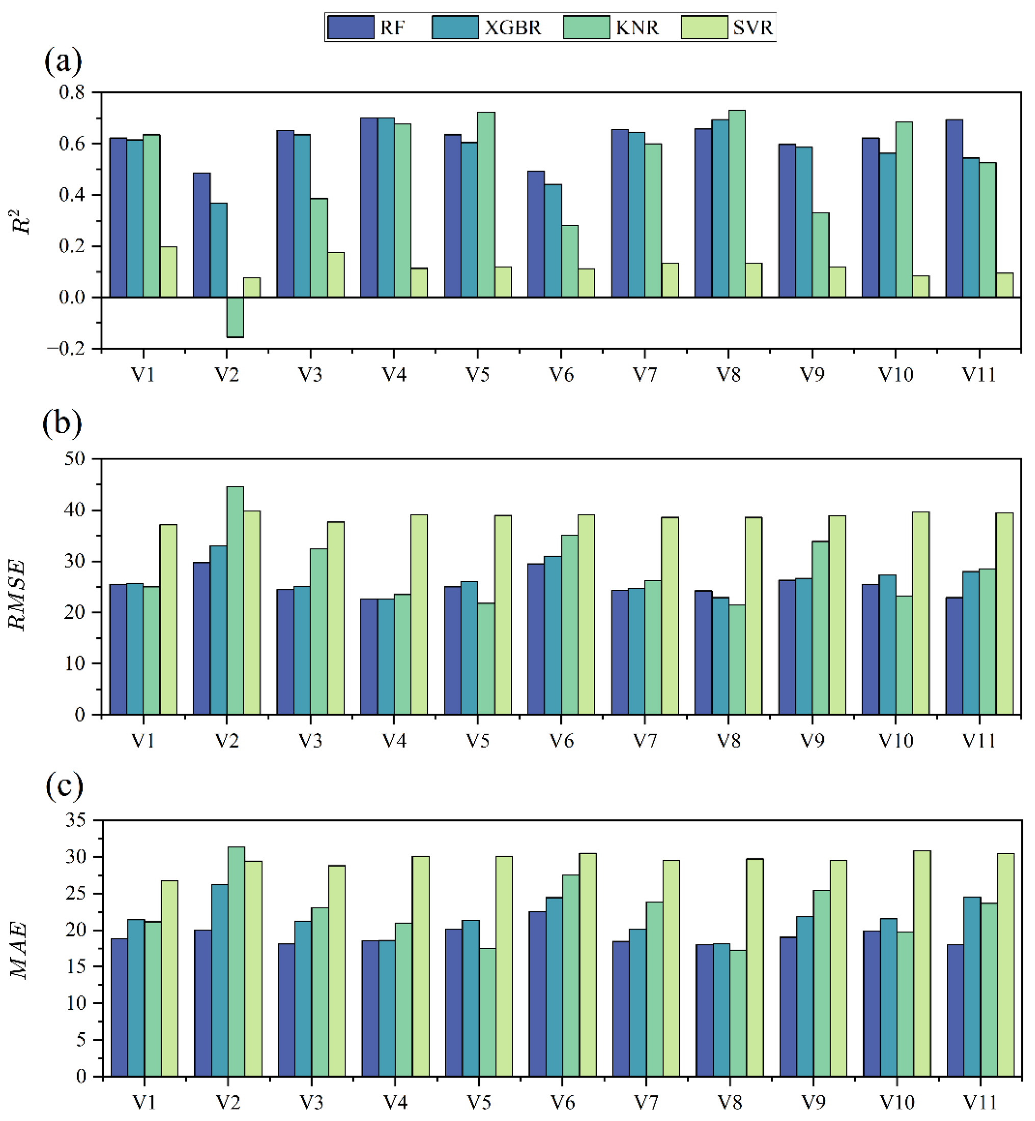
3.2.2. Multivariate Model Assessment

This study systematically assessed the performance of different variable combinations of NDTI, PCA_GLCM, VIs, and spectral bands for the AGB estimation of rubber plantations. V1 to V11 represent different variable combinations, respectively (

Table 6. Detailed combinations of different groups of variables.

Variable ID	Variable Combination
V1	NDTI, PCAGLCM
V2	NDTI, VIs
V3	NDTI, Spectral band
V4	PCAGLCM, VIs
V5	PCAGLCM, Spectral band
V6	VIs, Spectral band
V7	NDTI, PCAGLCM, VIs
V8	NDTI, PCAGLCM, Spectral band
V9	NDTI, VIs, Spectral band
V10	PCAGLCM, VIs, Spectral band
V11	NDTI, PCAGLCM, VIs, Spectral band

).

Figure 5 indicates the accuracy estimation of rubber forest AGB estimation models constructed with V1–V11 variable combinations and four machine learning regression techniques. The RF regression model achieved the highest precision in V4, with the parameters PCA_GLCM and VIs, resulting in an ${\mathrm{R}}^2$ value of 0.70. Additionally, V11 derived from NDTI, PCA_GLCM, VIs, and spectral band variables, also achieved a high precision, with an ${\mathrm{R}}^2$ value of 0.69. Similarly, the XGBR model obtained its highest precision in V4, with an ${\mathrm{R}}^2$ value of 0.70. The multivariate combination model received the highest estimation accuracy (${\mathrm{R}}^2$ = 0.73, RMSE = 21.48 t/ha, MAE = 17.25) in V8 of NDTI, PCA_GLCM, and spectral band parameters using the KNR. The SVR model achieved the lowest accuracy (${\mathrm{R}}^2$ < 0.2) in estimating rubber plantation AGB compared to the other three machine learning algorithms.

3.3. Model Evaluation of Different Methods for Screening Combinations of Important Variables

Figure 6 shows the importance of each type of remote sensing variable ranked from low to high. The top five most important parameters were used to estimate the AGB of the rubber plantation separately and were grouped as G1–G3. At the same time, the parameters were combined and NDTI parameters were added to estimate the AGB of the rubber plantation and were grouped as G4. Subsequently, all remote sensing variable combinations (VIs, Spectral band, and GLCM parameters) were used to select features using the Boruta feature screening method. After feature selection, NDTI was combined to form a feature set to estimate the AGB of the rubber plantation and was grouped as G5. Detailed information on the G1–G5 variable combinations is presented in

Table 7. Detailed combinations of G1–G5 groups of variables.

Variable ID	Parameters
G1	NDRE, NDWI, MSAVI, LSWI, EVI
G2	RE1, B, G, RE2, SWIR1
G3	PC5, PC1, PC8, PC6, PC2
G4	G1, G2, G3, NDTI
G5	ASMB, IMCORR1B, IMCORR2B, CORRG, CORRR, IMCORR1R, IMCORR2R, CORRRE1, SAVGRE1, CORRSWIR2, DISSSWIR2, IMCORR1SWIR2, IMCORR2SWIR2, B, G, RE1, RE2, SWIR1, SWIR2, NDRE; NDWI; MSAVI, NDTI

.

These results demonstrate that the rubber plantation AGB estimation accuracy is highest when the G5 is combined with machine learning models, while the estimation accuracy obtained using other feature combinations is lower than G5 (

Table 8. Assessment of model accuracy for different combinations of importance variables.

Variable ID	RF			XGBR			KNR			SVR
	${\mathbf{R}}^{\mathbf{2}}$	RMSE	MAE	${\mathbf{R}}^{\mathbf{2}}$	RMSE	MAE	${\mathbf{R}}^{\mathbf{2}}$	RMSE	MAE	${\mathbf{R}}^{\mathbf{2}}$	RMSE	MAE
G1	0.28	35.20	28.83	−0.16	44.64	39.45	0.36	33.25	27.15	−0.08	43.12	33.01
G2	0.56	27.62	22.84	0.37	32.89	25.34	0.59	26.61	21.35	0.21	36.80	28.67
G3	0.55	27.94	21.46	0.61	26.01	20.85	0.69	23.18	18.41	0.24	36.24	24.57
G4	0.67	23.86	19.19	0.64	24.77	19.09	0.65	24.46	20.18	0.11	39.18	29.84
G5	0.86	15.77	13.18	0.83	16.95	13.87	0.66	24.10	20.56	0.35	33.38	24.31

). Within the G5, the RF model combined with features selected using the Boruta method achieves the highest accuracy in estimating rubber plantation AGB, with an ${\mathrm{R}}^2$ of 0.86. Similarly, XGBR also achieved relatively high accuracy, with an ${\mathrm{R}}^2$ of 0.83. However, as depicted in Figure 7b,c, as well as Table 8, it is evident that the RMSE and MAE of XGBR on G5 are both higher than those of the RF model.

4. Discussion

4.1. Advantages of Integrating Multiple Variables with Machine Learning Techniques for AGB Estimation

The feature selection method combined with Sentinel-2 satellite data and machine learning algorithm has significantly improved the accuracy of estimating the AGB of Xishuangbanna rubber forest. Model validation conducted on different feature combinations using 20% of the dataset indicates a significant enhancement in AGB estimation accuracy after employing feature selection methods. By incorporating the G5 group parameters, the ${\mathrm{R}}^2$ value was found to be 0.86, with an RMSE of 15.77 Mg/ha and an MAE of 13.18 (Figure 7). Our study found that satisfactory accuracy can be achieved even without incorporating other parameters (such as SAR or/and LiDAR data) when using spectral bands, spectral indices, texture parameters, and texture indices. This conclusion was in agreement with the study of Bhumiphan et al. [20], who achieved an ${\mathrm{R}}^2$ of 0.79 and an RMSE of 29.42 kg/ha when estimating AGB in Thai rubber forests using Sentinel-2 satellite remote sensing data along with six vegetation indices and a stepwise multiple linear regression algorithm. The possible reasons could be attributed to (i) the use of modified Sentinel-2 satellite imagery (Harmonized Sentinel-2 MSI); (ii) parameter selection when using multiple remote sensing parameters; and (iii) the use of machine learning methods for estimating rubber forest AGB. In fact, Bhumiphan et al. [20] also emphasized, in their study, that the application of complex mathematical models such as machine learning can enhance the accuracy of rubber forest AGB estimation. In our study, the RF performed well in AGB estimation using remote sensing parameters. Our results indicate that non-parametric algorithms (RF, SVR, KNN, and XGBR) can better capture the complex relationship between rubber forest AGB and remote sensing variables by establishing nonlinear relationships between independent variables (features) and dependent variables (target variables) [33]. Additionally, combining GLCM features with spectral features can improve AGB estimation accuracy [5,66,67], which is consistent with our study.

4.2. Impact on Estimation Accuracy from Variables Optimization

This study extracted a total of 170 variables from Sentinel-2 satellite imagery, including 9 spectral bands, 7 vegetation indices, 153 texture parameters, and 1 texture index using the GEE platform. For the univariate machine learning model derived from four feature variables, GLCM achieved the highest accuracy, followed by spectral bands. The accuracy of vegetation indices in univariate AGB estimation is relatively poor, which may be attributed to two factors, as follows: (i) VIs tend to saturate when estimating AGB in high-density rubber plantations [68] and (ii) for spectral parameters relying on object surface hue or brightness calculations, texture parameters can more stably express spatial information, thus improving the estimation of rubber plantation AGB [69]. Additionally, research has shown that the selection of GLCM parameters can impact the accuracy of AGB estimation when using GLCM [10]. During variable combination, the combination of NDTI, PCA_GLCM, and spectral bands, along with the KNNR model, can effectively predict rubber plantation AGB.

For the spectral bands and vegetation indices, NDRE, NDWI, MSAVI, B, G, RE1, RE2, SWIR1, and SWIR2 are the relevant features selected by Boruta for predicting rubber plantation AGB, which yields similar results with Spearman’s correlation analysis (Figure 3). Our study indicates that, among spectral parameters, the red-edge spectral bands and their derived vegetation indices exhibit certain correlations with AGB, consistent with previous research findings [20]. Some GLCM texture parameters (such as ASM_B, CORR_R, SAVG_RE1, etc.) have been identified, using Boruta, as key features; Figure 5 also demonstrates the high contribution of GLCM features in AGB estimation. These results collectively indicate that texture parameters or spatial information contribute more significantly to the estimation of rubber plantation AGB than spectral bands and vegetation indices. Previous studies have shown that feature selection methods can significantly reduce overfitting, thereby enhancing generalization and improving model estimation accuracy, which aligns with our research findings [70].

The performance of four machine learning algorithms was evaluated with different feature selection methods for the AGB estimation of rubber plantations in this study. Extensive research demonstrates the robust performance of machine learning models in forest AGB estimation [8,27]. The results obtained after Boruta parameter selection indicate that RF regression performs the best (${\mathrm{R}}^2$ = 0.86, RMSE = 15.77 Mg/ha, MAE = 13.18), followed by XGBR, KNR ranking third, and SVR exhibiting the worst performance. This finding is in close agreement with the results of Singh et al. [71], who compared the performance of the Generalized Additive Mixed Model (GAMM), k Nearest Neighbor (k-NN), SVM, ANN, and RF for forest biomass estimation using Sentinel-2 data. They also found that the RF performed the best compared to other models. Similarly, Chen et al. [72] also demonstrated that the RF exhibited the best performance when combined with Sentinel-1 synthetic aperture radar (SAR), Sentinel-2 multispectral instrument (MSI), and SRTM digital elevation model (DEM) data with stepwise regression (SWR), geographically weighted regression (GWR), ANN, SVR, and RF algorithms to establish an optimal forest AGB model, which is consistent with our findings.

4.3. Limitations and Potential Applications

The Sentinel-2 data was combined with four ML techniques and various variable selection strategies to estimate rubber plantation AGB, aiming to explore the optimal variables for AGB estimation within Sentinel-2 imagery data. Through the parameter selection method Boruta, different spectral bands, spectral parameters, and GLCM parameters were selected, resulting in a satisfactory estimation accuracy (${\mathrm{R}}^2$ = 0.86). Although this study achieved a promising predictive accuracy in estimating rubber plantation AGB, we did not evaluate the performance of the combination of spectral information, texture features, and PALSAR satellite data (such as HH and HV). Previous studies indicated that the inclusion of PALSAR can enhance the accuracy of forest AGB estimation [73], but whether the optimized feature parameters derived from PALSAR improve AGB estimation remains unclear. Additionally, elevation, aspect, slope, and other terrain factors, as well as stand age, are also important parameters applied in the estimation of rubber plantation AGB [8,32,74]. Therefore, the parameter optimization approach should be further evaluated using different satellite data, as well as terrain factors and stand age parameters in rubber plantation AGB estimation in the future.

Although this study established an optimal AGB estimation model with variable optimization across different varieties and planting years of rubber plantations using limited sampling data, further evaluation is needed for the independent testing of variety and age effects. Given the differences and imbalance among the samples, the 24 samples collected in 2021 and 40 samples from 2023 were pooled. The merged 64 samples were split into 80% for the training dataset and 20% for the testing dataset with random stratified sampling. Even though a repeated resampling method of 10-fold cross-validation was employed to enhance the model’s robustness, the limited sample size (64 samples) may result in instability in model fitting accuracy for variable optimization, due to insufficient sample points. In addition, the latest study suggested that at least 100 sample points are needed for building a single tree species biomass predictive model [75]. This implies that collecting a more diverse range of samples is critical for enhancing the estimation accuracy and transferability of the model, which inevitably requires additional costs and resources for field surveys. Fortunately, the existing research has proven that UAVs equipped with demand sensors are a beneficial alternative to field surveys [76]. Especially in field investigations for gathering AGB, LiDAR (Light Detection and Ranging) sensors mounted on UAVs show great potential in collecting forest plot-level data at a regional scale. This will provide practical applications for utilizing regionally scaled field data to construct a variable-optimized stable model for estimating forest biophysical parameters in large-scale regions.

5. Conclusions

This study systematically evaluated the impact of various feature selection methods combined with multiple features extracted from Sentinel-2 remote sensing data obtained from the GEE platform coupled with four machine learning techniques on the estimation of rubber plantation AGB. The results demonstrate that RF combined with the Boruta feature selection method achieved the highest accuracy for AGB estimation in rubber plantations (${\mathrm{R}}^2$ = 0.86, RMSE = 15.77 Mg/ha) compared to other machine learning regression algorithms. This implied that employing appropriate feature selection methods can significantly improve the AGB estimation accuracy of rubber plantations when using a large number of parameters, thereby aiding in the rapid assessment of productivity and carbon storage in rubber plantations. This research provides new insights into accurately estimating other biophysical parameters of other crops by considering optimized variables derived from a large amount of feature parameters.

References

1. Cornish, K. Similarities and differences in rubber biochemistry among plant species. Phytochemistry 2001, 57, 1123–1134. [Google Scholar] [CrossRef] [PubMed]
2. Yang, X.; Blagodatsky, S.; Liu, F.; Beckschäfer, P.; Xu, J.; Cadisch, G. Rubber tree allometry, biomass partitioning and carbon stocks in mountainous landscapes of sub-tropical China. For. Ecol. Manag. 2017, 404, 84–99. [Google Scholar] [CrossRef]
3. Chen, B.; Xiao, X.; Wu, Z.; Yun, T.; Kou, W.; Ye, H.; Lin, Q.; Doughty, R.; Dong, J.; Ma, J.; et al. Identifying establishment year and pre-conversion land cover of rubber plantations on Hainan Island, China using Landsat data during 1987–2015. Remote Sens. 2018, 10, 1240. [Google Scholar] [CrossRef]
4. Tang, J.; Pang, J.; Chen, M.; Guo, X.; Zeng, R. Biomass and its estimation model of rubber plantations in Xishuangbanna, Southwest China. Chin. J. Ecol. 2009, 28, 1942–1948. [Google Scholar]
5. Charoenjit, K.; Zuddas, P.; Allemand, P.; Pattanakiat, S.; Pachana, K. Estimation of biomass and carbon stock in Para rubber plantations using object-based classification from Thaichote satellite data in Eastern Thailand. J. Appl. Remote Sens. 2015, 9, 096072. [Google Scholar] [CrossRef]
6. Wu, Y.; Ou, G.; Lu, T.; Huang, T.; Zhang, X.; Liu, Z.; Yu, Z.; Guo, B.; Wang, E.; Feng, Z. Improving Aboveground Biomass Estimation in Lowland Tropical Forests across Aspect and Age Stratification: A Case Study in Xishuangbanna. Remote Sens. 2024, 16, 1276. [Google Scholar] [CrossRef]
7. Zhang, X.; Ni-meister, W. Remote Sensing of Forest Biomass. In Biophysical Applications of Satellite Remote Sensing; Hanes, J.M., Ed.; Springer: Berlin/Heidelberg, Germany, 2014; pp. 63–98. [Google Scholar]
8. Chen, B.; Yun, T.; Ma, J.; Kou, W.; Li, H.; Yang, C.; Xiao, X.; Zhang, X.; Sun, R.; Xie, G.; et al. High-Precision Stand Age Data Facilitate the Estimation of Rubber Plantation Biomass: A Case Study of Hainan Island, China. Remote Sens. 2020, 12, 3853. [Google Scholar] [CrossRef]
9. Ploton, P.; Barbier, N.; Couteron, P.; Antin, C.M.; Ayyappan, N.; Balachandran, N.; Barathan, N.; Bastin, J.F.; Chuyong, G.; Dauby, G.; et al. Toward a general tropical forest biomass prediction model from very high resolution optical satellite images. Remote Sens. Environ. 2017, 200, 140–153. [Google Scholar] [CrossRef]
10. Liang, Y.; Kou, W.; Lai, H.; Wang, J.; Wang, Q.; Xu, W.; Wang, H.; Lu, N. Improved estimation of aboveground biomass in rubber plantations by fusing spectral and textural information from UAV-based RGB imagery. Ecol. Indic. 2022, 142, 109286. [Google Scholar] [CrossRef]
11. Panagiotidis, D.; Abdollahnejad, A.; Slavík, M. 3D point cloud fusion from UAV and TLS to assess temperate managed forest structures. Int. J. Appl. Earth Obs. Geoinf. 2022, 112, 102917. [Google Scholar] [CrossRef]
12. González-Jaramillo, V.; Fries, A.; Bendix, J. AGB estimation in a tropical mountain forest (TMF) by means of RGB and multispectral images using an unmanned aerial vehicle (UAV). Remote Sens. 2019, 11, 1413. [Google Scholar] [CrossRef]
13. Ni, W.; Dong, J.; Sun, G.; Zhang, Z.; Pang, Y.; Tian, X.; Li, Z.; Chen, E. Synthesis of leaf-on and leaf-off unmanned aerial vehicle (UAV) stereo imagery for the inventory of aboveground biomass of deciduous forests. Remote Sens. 2019, 11, 889. [Google Scholar] [CrossRef]
14. Yang, G.; Liu, J.; Zhao, C.; Li, Z.; Huang, Y.; Yu, H.; Xu, B.; Yang, X.; Zhu, D.; Zhang, X.; et al. Unmanned aerial vehicle remote sensing for field-based crop phenotyping: Current status and perspectives. Front. Plant Sci. 2017, 8, 1111. [Google Scholar] [CrossRef] [PubMed]
15. Pratama, L.D.Y.; Danoedoro, P. Above-ground carbon stock estimates of rubber (hevea brasiliensis) using Sentinel 2A imagery: A case study in rubber plantation of PTPN IX Kebun Getas and Kebun Ngobo, Semarang Regency. IOP Conf. Ser. Earth Environ. Sci. 2020, 500, 012087. [Google Scholar] [CrossRef]
16. Yasen, K.; Koedsin, W. Estimating aboveground biomass of rubber tree using remote sensing in Phuket Province, Thailand. J. Med. Bioeng. 2015, 4, 451–456. [Google Scholar] [CrossRef]
17. Azizan, F.A.; Kiloes, A.M.; Astuti, I.S.; Abdul Aziz, A. Application of optical remote sensing in rubber plantations: A systematic review. Remote Sens. 2021, 13, 429. [Google Scholar] [CrossRef]
18. Wang, Y.; Pang, Y.; Shu, Q. Counter-estimation on aboveground biomass of Hevea brasiliensis plantation by remote sensing with random forest algorithm-a case study of Jinghong. J. Southwest For. Univ. 2013, 33, 38–45. [Google Scholar]
19. Gao, S.; Zhong, R.; Yan, K.; Ma, X.; Chen, X.; Pu, J.; Gao, S.; Qi, J.; Yin, G.; Myneni, R.B. Evaluating the saturation effect of vegetation indices in forests using 3D radiative transfer simulations and satellite observations. Remote Sens. Environ. 2023, 295, 113665. [Google Scholar] [CrossRef]
20. Bhumiphan, N.; Nontapon, J.; Kaewplang, S.; Srihanu, N.; Koedsin, W.; Huete, A. Estimation of rubber yield using Sentinel-2 satellite data. Sustainability 2023, 15, 7223. [Google Scholar] [CrossRef]
21. Zhang, L.; Zhang, X.; Shao, Z.; Jiang, W.; Gao, H. Integrating Sentinel-1 and 2 with LiDAR data to estimate aboveground biomass of subtropical forests in northeast Guangdong, China. Int. J. Digit. Earth 2023, 16, 158–182. [Google Scholar] [CrossRef]
22. Bar, S.; Parida, B.R.; Pandey, A.C. Landsat-8 and Sentinel-2 based Forest fire burn area mapping using machine learning algorithms on GEE cloud platform over Uttarakhand, Western Himalaya. Remote Sens. Appl. Soc. Environ. 2020, 18, 100324. [Google Scholar] [CrossRef]
23. Chen, B.; Xiao, X.; Li, X.; Pan, L.; Doughty, R.; Ma, J.; Dong, J.; Qin, Y.; Zhao, B.; Wu, Z. A mangrove forest map of China in 2015: Analysis of time series Landsat 7/8 and Sentinel-1A imagery in Google Earth Engine cloud computing platform. ISPRS J. Photogramm. Remote Sens. 2017, 131, 104–120. [Google Scholar] [CrossRef]
24. Abdollahnejad, A.; Panagiotidis, D. Tree Species Classification and Health Status Assessment for a Mixed Broadleaf-Conifer Forest with UAS Multispectral Imaging. Remote Sens. 2020, 12, 3722. [Google Scholar] [CrossRef]
25. Taddese, H.; Asrat, Z.; Burud, I.; Gobakken, T.; Ørka, H.O.; Dick, Ø.B.; Næsset, E. Use of remotely sensed data to enhance estimation of aboveground biomass for the dry Afromontane forest in South-Central Ethiopia. Remote Sens. 2020, 12, 3335. [Google Scholar] [CrossRef]
26. Xu, F.; Chen, W.; Xie, R.; Wu, Y.; Jiang, D. Vegetation Classification and a Biomass Inversion Model for Wildfires in Chongli Based on Remote Sensing Data. Fire 2024, 7, 58. [Google Scholar] [CrossRef]
27. Lourenço, P.; Godinho, S.; Sousa, A.; Gonçalves, A.C. Estimating tree aboveground biomass using multispectral satellite-based data in Mediterranean agroforestry system using random forest algorithm. Remote Sens. Appl. Soc. Environ. 2021, 23, 100560. [Google Scholar] [CrossRef]
28. Fu, Y.; Yang, G.; Song, X.; Li, Z.; Xu, X.; Feng, H.; Zhao, C. Improved estimation of winter wheat aboveground biomass using multiscale textures extracted from UAV-based digital images and hyperspectral feature analysis. Remote Sens. 2021, 13, 581. [Google Scholar] [CrossRef]
29. Zheng, H.; Cheng, T.; Zhou, M.; Li, D.; Yao, X.; Tian, Y.; Cao, W.; Zhu, Y. Improved estimation of rice aboveground biomass combining textural and spectral analysis of UAV imagery. Precis. Agric. 2018, 20, 611–629. [Google Scholar] [CrossRef]
30. Hsu, H.-H.; Hsieh, C.-W.; Lu, M.-D. Hybrid feature selection by combining filters and wrappers. Expert Syst. Appl. 2011, 38, 8144–8150. [Google Scholar] [CrossRef]
31. Huang, N.; Li, R.; Lin, L.; Yu, Z.; Cai, G. Low redundancy feature selection of short term solar irradiance prediction using conditional mutual information and Gauss process regression. Sustainability 2018, 10, 2889. [Google Scholar] [CrossRef]
32. Zhang, Y.; Liu, J.; Li, W.; Liang, S. A proposed ensemble feature selection method for estimating forest aboveground biomass from multiple satellite data. Remote Sens. 2023, 15, 1096. [Google Scholar] [CrossRef]
33. Lu, D.; Chen, Q.; Wang, G.; Liu, L.; Li, G.; Moran, E. A survey of remote sensing-based aboveground biomass estimation methods in forest ecosystems. Int. J. Digit. Earth 2014, 9, 63–105. [Google Scholar] [CrossRef]
34. Ghosh, S.M.; Behera, M.D. Aboveground biomass estimation using multi-sensor data synergy and machine learning algorithms in a dense tropical forest. Appl. Geogr. 2018, 96, 29–40. [Google Scholar] [CrossRef]
35. Shin, J.; Jeong, S.; Chang, D.Y. Estimation of forest carbon stock in South Korea using machine learning with high-resolution remote sensing data. Atmosphere 2023, 33, 61–72. [Google Scholar] [CrossRef]
36. Vega Isuhuaylas, L.A.; Hirata, Y.; Ventura Santos, L.C.; Serrudo Torobeo, N. Natural forest mapping in the Andes (Peru): A comparison of the performance of machine-learning algorithms. Remote Sens. 2018, 10, 782. [Google Scholar] [CrossRef]
37. Zhang, J.; Huang, Y.; Pu, R.; Gonzalez-Moreno, P.; Yuan, L.; Wu, K.; Huang, W. Monitoring plant diseases and pests through remote sensing technology: A review. Comput. Electron. Agric. 2019, 165, 104943. [Google Scholar] [CrossRef]
38. Trisasongko, B.H.; Panuju, D.R.; Sholihah, R.; Karyati, N.E. Estimating the girth distribution of rubber trees using support and relevance vector machines. Appl. Geomat. 2024, 16, 337–345. [Google Scholar] [CrossRef]
39. Tian, Y.; Huang, H.; Zhou, G.; Zhang, Q.; Tao, J.; Zhang, Y.; Lin, J. Aboveground mangrove biomass estimation in Beibu Gulf using machine learning and UAV remote sensing. Sci. Total Environ. 2021, 781, 146816. [Google Scholar] [CrossRef]
40. Zhang, X.; Shen, H.; Huang, T.; Wu, Y.; Guo, B.; Liu, Z.; Luo, H.; Tang, J.; Zhou, H.; Wang, L.; et al. Improved random forest algorithms for increasing the accuracy of forest aboveground biomass estimation using Sentinel-2 imagery. Ecol. Indic. 2024, 159, 111752. [Google Scholar] [CrossRef]
41. Lu, N.; Wang, W.H.; Zhang, Q.F.; Li, D.; Yao, X.; Tian, Y.C.; Zhu, Y.; Cao, W.X.; Baret, R.; Liu, S.Y.; et al. Estimation of nitrogen nutrition status in winter wheat from unmanned aerial vehicle based multi-angular multispectral imagery. Front. Plant Sci. 2019, 10, 1601. [Google Scholar] [CrossRef]
42. Su, L.J.; Wen, T.Y.; Tao, W.H.; Deng, M.J.; Yuan, S.; Zeng, S.L.; Wang, Q.J. Growth indexes and yield prediction of summer maize in China based on supervised machine learning method. Agronomy 2023, 13, 132. [Google Scholar] [CrossRef]
43. Kou, W.; Dong, J.; Xiao, X.; Hernandez, A.J.; Qin, Y.; Zhang, G.; Chen, B.; Lu, N.; Doughty, R. Expansion dynamics of deciduous rubber plantations in Xishuangbanna, China during 2000–2010. GISci. Remote Sens. 2018, 55, 905–925. [Google Scholar] [CrossRef]
44. Xu, W.; Feng, Z.; Su, Z.; Xu, H.; Jiao, Y.; Fan, J. Development and experiment of handheld digitalized and multi-functional forest measurement gun. Trans. Chin. Soc. Agric. Eng. 2013, 29, 90–99. [Google Scholar]
45. Main-Knorn, M.; Pflug, B.; Louis, J.; Debaecker, V.; Müller-Wilm, U.; Gascon, F. Sen2Cor for Sentinel-2; SPIE: Bellingham, WA, USA, 2017; Volume 10427. [Google Scholar]
46. Dong, J.; Xiao, X.; Chen, B.; Torbick, N.; Jin, C.; Zhang, G.; Biradar, C. Mapping deciduous rubber plantations through integration of PALSAR and multi-temporal Landsat imagery. Remote Sens. Environ. 2013, 134, 392–402. [Google Scholar] [CrossRef]
47. Linjing Zhang, Z.S.Z.W. Estimation of forest aboveground biomass using the integration of spectral and textural features from GF-1 satellite image. In Proceedings of the 2016 4th International Workshop on Earth Observation and Remote Sensing Applications (EORSA), Guangzhou, China, 4–6 July 2016; pp. 353–357. [Google Scholar] [CrossRef]
48. Tucker, C.J. Red and photographic infrared linear combinations for monitoring vegetation. Remote Sens. Environ. 1979, 8, 127–150. [Google Scholar] [CrossRef]
49. Huete, A.; Didan, K.; Miura, T.; Rodriguez, E.P.; Gao, X.; Ferreira, L.G. Overview of the radiometric and biophysical performance of the MODIS vegetation indices. Remote Sens. Environ. 2002, 83, 195–213. [Google Scholar] [CrossRef]
50. Rouse, J.W.; Haas, R.H.; Schell, J.A.; Deering, D.W. Monitoring vegetation systems in the Great Plains with ERTS. NASA Spec. Publ. 1974, 351, 309. [Google Scholar]
51. McFeeters, S.K. The use of the Normalized Difference Water Index (NDWI) in the delineation of open water features. Int. J. Remote Sens. 1996, 17, 1425–1432. [Google Scholar] [CrossRef]
52. Chandrasekar, K.; Sesha Sai, M.; Roy, P.; Dwevedi, R. Land Surface Water Index (LSWI) response to rainfall and NDVI using the MODIS Vegetation Index product. Int. J. Remote Sens. 2010, 31, 3987–4005. [Google Scholar] [CrossRef]
53. Fitzgerald, G.; Rodriguez, D.; O’Leary, G. Measuring and predicting canopy nitrogen nutrition in wheat using a spectral index—The canopy chlorophyll content index (CCCI). Field Crops Res. 2010, 116, 318–324. [Google Scholar] [CrossRef]
54. Qi, J.; Chehbouni, A.; Huete, A.R.; Kerr, Y.H.; Sorooshian, S. A modified soil adjusted vegetation index. Remote Sens. Environ. 1994, 48, 119–126. [Google Scholar] [CrossRef]
55. Haralick, R.M.; Shanmugam, K.; Dinstein, I.H. Textural features for image classification. IEEE Trans. Syst. Man Cybern. 1973, SMC-3, 610–621. [Google Scholar] [CrossRef]
56. Conners, R.W.; Trivedi, M.M.; Harlow, C.A. Segmentation of a high-resolution urban scene using texture operators. Comput. Vis. Graph. Image Process. 1984, 25, 273–310. [Google Scholar] [CrossRef]
57. Segal, M.R. Machine learning benchmarks and random forest regression. Cent. Bioinform. Mol. Biostat. 2004, 1–14. [Google Scholar]
58. Chen, T.; Guestrin, C. Xgboost: A scalable tree boosting system. In Proceedings of the 22nd Acm Sigkdd International Conference on Knowledge Discovery and Data Mining, San Francisco, CA, USA, 13–17 August 2016; pp. 785–794. [Google Scholar] [CrossRef]
59. Bishop, C.M. Pattern Recognition and Machine Learning; Springer: Berlin/Heidelberg, Germany, 2006; Volume 2, pp. 5–43. [Google Scholar] [CrossRef]
60. Cortes, C.; Vapnik, V. Support-vector networks. Mach. Learn. 1995, 20, 273–297. [Google Scholar] [CrossRef]
61. Weerts, H.J.; Mueller, A.C.; Vanschoren, J. Importance of tuning hyperparameters of machine learning algorithms. arXiv 2020, arXiv:2007.07588. [Google Scholar] [CrossRef]
62. Machidon, A.L.; Del Frate, F.; Picchiani, M.; Machidon, O.M.; Ogrutan, P.L. Geometrical Approximated Principal Component Analysis for Hyperspectral Image Analysis. Remote Sens. 2020, 12, 1698. [Google Scholar] [CrossRef]
63. Li, X.; Wang, Y.; Basu, S.; Kumbier, K.; Yu, B. A debiased MDI feature importance measure for random forests. Adv. Neural Inf. Process. Syst. 2019, 32, 8049–8059. [Google Scholar] [CrossRef]
64. Kursa, M.B.; Rudnicki, W.R. Feature selection with the Boruta package. J. Stat. Softw. 2010, 36, 1–13. [Google Scholar] [CrossRef]
65. Degenhardt, F.; Seifert, S.; Szymczak, S. Evaluation of variable selection methods for random forests and omics data sets. Brief. Bioinform. 2019, 20, 492–503. [Google Scholar] [CrossRef]
66. Lu, D. Aboveground biomass estimation using Landsat TM data in the Brazilian Amazon. Int. J. Remote Sens. 2005, 26, 2509–2525. [Google Scholar] [CrossRef]
67. Karlson, M.; Ostwald, M.; Reese, H.; Sanou, J.; Tankoano, B.; Mattsson, E. Mapping tree canopy cover and aboveground biomass in Sudano-Sahelian woodlands using Landsat 8 and random forest. Remote Sens. 2015, 7, 10017–10041. [Google Scholar] [CrossRef]
68. Samanta, A.; Knyazikhin, Y.; Xu, L.; Dickinson, R.E.; Fu, R.; Costa, M.H.; Saatchi, S.S.; Nemani, R.R.; Myneni, R.B. Seasonal changes in leaf area of Amazon forests from leaf flushing and abscission. J. Geophys. Res. Biogeosci. 2012, 117, 1–13. [Google Scholar] [CrossRef]
69. Zhang, C.; Huang, C.; Li, H.; Liu, Q.; Liu, G. Effect of textural features in remote sensed data on rubber plantation extraction at different levels of spatial resolution. Forests 2020, 11, 399. [Google Scholar] [CrossRef]
70. Yu, H.; Wu, Y.; Niu, L.; Chai, Y.; Feng, Q.; Wang, W.; Liang, T. A method to avoid spatial overfitting in estimation of grassland above-ground biomass on the Tibetan Plateau. Ecol. Indic. 2021, 125, 107450. [Google Scholar] [CrossRef]
71. Singh, C.; Karan, S.K.; Sardar, P.; Samadder, S.R. Remote sensing-based biomass estimation of dry deciduous tropical forest using machine learning and ensemble analysis. J. Environ. Manag. 2022, 308, 114639. [Google Scholar] [CrossRef]
72. Chen, L.; Wang, Y.; Ren, C.; Zhang, B.; Wang, Z. Optimal combination of predictors and algorithms for forest above-ground biomass mapping from Sentinel and SRTM data. Remote Sens. 2019, 11, 414. [Google Scholar] [CrossRef]
73. Sinha, S.; Jeganathan, C.; Sharma, L.; Nathawat, M.; Das, A.K.; Mohan, S. Developing synergy regression models with space-borne ALOS PALSAR and Landsat TM sensors for retrieving tropical forest biomass. J. Earth Syst. Sci. 2016, 125, 725–735. [Google Scholar] [CrossRef]
74. Rejou-Mechain, M.; Muller-Landau, H.C.; Detto, M.; Thomas, S.C.; Le Toan, T.; Saatchi, S.S.; Barreto-Silva, J.S.; Bourg, N.A.; Bunyavejchewin, S.; Butt, N. Local spatial structure of forest biomass and its consequences for remote sensing of carbon stocks. Biogeosciences 2014, 11, 6827–6840. [Google Scholar] [CrossRef]
75. Yan, X.; Li, J.; Smith, A.R.; Yang, D.; Ma, T.; Su, Y.; Shao, J. Evaluation of machine learning methods and multi-source remote sensing data combinations to construct forest above-ground biomass models. Int. J. Digit. Earth 2023, 16, 4471–4491. [Google Scholar] [CrossRef]
76. Zhou, X.; Yang, L.; Wang, W.; Chen, B. UAV Data as an Alternative to Field Sampling to Monitor Vineyards Using Machine Learning Based on UAV/Sentinel-2 Data Fusion. Remote Sens. 2021, 13, 457. [Google Scholar] [CrossRef]
Figure 1. The overview of the sampling area. (a) Locations of the sampling area, DEM was obtained from https://www.earthdata.nasa.gov/ (accessed on 18 February 2023); (b) the growth status of rubber forests within the sampling area; (c) the diameter at breast height (DBH) measurement in field survey; and (d) RGB imagery of a sampling plot derived from UAV.
Forests 15 00900 g001
Figure 2. The workflow of AGB estimation of rubber plantations in this study.
Forests 15 00900 g002
Figure 3. Spearman’s correlation analysis for the relationships between remote sensing variables and the measured AGB of rubber plantations, (a) spectral band; (b) VIs.. Data with an asterisk (*) have a p-value ≤ 0.05. B represents Blue band, G represents Green band, and R represents Red band. RE1, RE2, and RE3 represent red edge band 1, red edge band 2, and red edge band 3, respectively.
Forests 15 00900 g003
Figure 4. Analysis of PCA. (a) Explained variance using PCA based on texture parameter; (b) Spearman’s correlation analysis for the relationships between PCA based on texture parameter computation and the measured AGB of rubber plantations. Data with an asterisk (*) have a p-value ≤ 0.05.
Forests 15 00900 g004
Figure 5. Comparison of the accuracy of variable combination estimation of forest AGB in machine learning. (a) R 2 of each model for each group of features; (b) RMSE of each model for each group of features; (c) MAE of each model for each group of features.
Forests 15 00900 g005
Figure 6. Assessment of the importance of different parameter types: (a) assessment of the importance of 10 PCAs obtained based on GLCM parameters; (b) assessment of the importance of spectral parameters; and (c) assessment of the importance of VIs.
Forests 15 00900 g006
Figure 7. Assessment of model accuracy for five different combinations of variable characteristics screening, G1–G5 are different combinations of variables. (a) R 2 of the model; (b) RMSE of the model; (c) MAE of the model.
Forests 15 00900 g007