Article

A New Remote Sensing Index for Forest Dryness Monitoring Using Multi-Spectral Satellite Imagery

by
Thai Son Le
1,2,
Bernard Dell
1,3,* and
Richard Harper
1
1
Agriculture and Forest Sciences, Murdoch University, Perth, WA 6150, Australia
2
Department of Environmental Management, Vietnam National University of Forestry, Hanoi 13417, Vietnam
3
Forest Protection Research Centre, Vietnamese Academy of Forest Sciences, Hanoi 11910, Vietnam
*
Author to whom correspondence should be addressed.
Forests 2024, 15(6), 915; https://doi.org/10.3390/f15060915 (registering DOI)
Submission received: 16 April 2024 / Revised: 15 May 2024 / Accepted: 23 May 2024 / Published: 24 May 2024
(This article belongs to the Special Issue Monitoring Forest Change Dynamic with Remote Sensing)

Abstract

:
Canopy water content is a fundamental indicator for assessing the level of plant water stress. The correlation between changes in water content and the spectral reflectance of plant leaves at near-infrared (NIR) and short-wave infrared (SWIR) wavelengths forms the foundation for developing a new remote sensing index, the Infrared Canopy Dryness Index (ICDI), to monitor forest dryness that can be used to predict the consequences of water stress. This study introduces the index, that uses spectral reflectance analysis at near-infrared wavelengths, encapsulated by the Normalized Difference Infrared Index (NDII), in conjunction with specific canopy conditions as depicted by the widely recognized Normalized Difference Vegetation Index (NDVI). Development of the ICDI commenced with the construction of an NDII/NDVI feature space, inspired by a conceptual trapezoid model. This feature space was then parameterized, and the spatial region indicative of water stress conditions, referred to as the dry edge, was identified based on the analysis of 10,000 random observations. The ICDI was produced from the combination of the vertical distance (i.e., under consistent NDVI conditions) from an examined observation to the dry edge. Comparisons between data from drought-affected and non-drought-affected control plots in the Australian Northern Jarrah Forest affirmed that the ICDI effectively depicted forest dryness. Moreover, the index was able to detect incipient water stress several months before damage from an extended drought and heatwave. Using freely available satellite data, the index has potential for broad application in monitoring the onset of forest dryness. This will require validation of the ICDI in diverse forest systems to quantify the efficacy of the index.

1. Introduction

The Earth’s climate is undergoing rapid changes, evident in the increases in global temperatures and shifts in hydrological processes within watersheds [1,2,3]. Notably, a significant decline in mean rainfall, coupled with the heightened water demand of ecosystems in response to rising temperatures, has diminished water storage in many watersheds. A clear indicator of this transformation is the depletion of soil water and groundwater stores and availability to vegetation [3,4]. Consequently, water stress in forest ecosystems is becoming more prevalent, leading to detrimental effects on trees ranging from dehydration and wilting to mortality [5,6,7]. Climate change also exacerbates the severity and likelihood of droughts and heat waves, amplifying the risks and impacts of water stress [2,8].
Forest water stress occurs when a forest undergoes an extended or intense shortage of water that raises the dryness of the canopies to a certain level, which depends on tree species. This condition triggers physiological and ecological reactions that may adversely impact the health and productivity of the forest [4,9,10]. The increasing prevalence of water stress presents a significant threat to the health and resilience of forest ecosystems [9], underscoring the imperative for comprehensive strategies to alleviate the impacts of climate change on these ecosystems and associated water resources [10,11,12,13]. A wealth of research has highlighted that minimizing exposed canopy area and leaf area, thereby lowering a tree’s water use, is an effective strategy for coping with increasing forest dryness [14,15]. Given that forestry interventions entail significant expenses, a key requirement is the prompt identification and delineation of potential water stress hotspots within forests so that forest managers can implement effective interventions, such as thinning operations [16,17]. However, typical field measurements for forest dryness at the forest scale have faced challenges, particularly in providing a spatially comprehensive description of this phenomenon. To overcome these obstacles, remote sensing could provide a more rapid and effective approach [9].
Many remote sensing indices have been devised to assess water content in plants, serving as partial indicators of water stress [18,19,20,21,22], among which the Normalized Difference Water Index (NDWI) [23] was particularly favored in the late 2000s. However, in expansive forests comprising individuals with varying canopy conditions, data on water content alone may not conclusively depict water stress. Hence, the condition of the tree canopy is an essential factor that must be considered. Building on this understanding, some researchers have employed trapezoidal models to delineate the correlation between vegetation water indices and canopy cover, leading to the introduction of new methods [24,25,26]. However, indices that leverage the Land Surface Temperature (LST)–NDVI relationship often yield biased results in areas with damaged vegetation, bare soil and exposed rock [12,25,27,28,29]. Other studies have shown that the use of low spatial resolution imagery, such as from MODIS (Moderate Resolution Imaging Spectroradiometer), may hinder effective hotspot analysis [20,30,31]. Hence, there is a pressing need to establish a more robust and sensitive satellite-based method to detect the early onset of dryness in forest canopies, leading to water stress, and in some cases tree deaths.
A primary indicator of water deficit in trees is the reduction in water content [11,32,33,34,35], particularly in the upper canopy, which is directly exposed to sunlight. Consequently, one of the fundamental approaches for detecting vegetation water stress involves the utilization of spectral reflectance at short-wave infrared wavelengths (SWIR) [21,22,36,37]. Additionally, the detection of vegetation, typically represented through near-infrared (NIR) spectral reflectance, is crucial in distinguishing it from other types of land cover [30,38,39]. SWIR reflectance has been used to evaluate plant water content, observing an increase in SWIR reflectance as leaf water content decreases, and vice versa [18,22,35,36,40,41]. The difference in spectral reflectance between NIR and SWIR regions can provide valuable information due to the differential absorption and reflection of these two wavebands by various components in leaves [42]. The degree of SWIR reflectance is closely linked to the water content in the canopy, especially for the band from 1600 to 2500 nm [40,43,44]. Nonetheless, factors such as non-pigment dry matter content can also affect SWIR reflectance [18,45,46]. Since NIR is primarily influenced by dry matter content [47,48], subtracting NIR from SWIR can help mitigate these effects, thereby enhancing the accuracy of water content estimation in leaves [20,48].
The basic method for estimating water content in the tree canopy involves normalized difference indices of the form: (NIR − SWIR)/(NIR + SWIR). However, each remote sensing system employs sensors with varying bandwidths and locations. The NIR band (0.7–1 μm) is relatively consistent among sensors due to its narrow range. In contrast, the SWIR band (1–3 μm) is broader and more varied, with some remote sensing systems capturing two or more SWIR bands with different characteristics. For instance, Landsat TM provides bands 5 and 7, while MODIS offers bands 5, 6, and 7. Consequently, the normalized difference index of NIR and SWIR may differ based on the specific sensor/SWIR band used in the equation. To streamline the multitude of similar normalized difference NIR-SWIR indices with varying nomenclature but identical scientific intent, Ji et al. [43] consolidated these spectral indices into three primary categories, based on the SWIR wavelength captured, regardless of the sensor. These are: (1) Normalized Difference Water Index (NDWI) [23], utilizing the short region of the SWIR wavelength (1.23–1.25 μm); (2) Normalized Difference Infrared Index (NDII) [22], using the medium region of the SWIR wavelength (1.55–1.75 μm); and (3) Normalized Burn Ratio (NBR) [49], employing the long region of the SWIR wavelength (2.05–2.45 μm). Among these, the NDWI and the NDII are more commonly used for estimating plant water content [43,44,50,51].
In times of diminishing soil water availability, the canopy water content (CWC) declines [43,51]. The relationship between CWC and canopy cover can be simplified as in Figure 1, to reveal the potential for utilizing these parameters to effectively convey the water stress conditions in plants. In this context, the term “dry edge” refers to conditions characterized by limited soil water availability, whereas the “wet edge” denotes situations with unrestricted access to soil water.
Under water deficit, the canopy water content diminishes significantly, leading to wilting and a marked increase in SWIR spectral reflectance. In contrast, NIR reflectance tends to be more stable under these conditions, as there is minimal variation in the dry matter content, pigmentation, and leaf structure during the initial stages of water stress [48]. Thus, this subtle interaction between NIR and SWIR reflectance offers critical insights into the water status of plants. A larger disparity between these two reflectance values typically indicates a more severe water deficit in the tree canopy [43,48]. This understanding is instrumental in the remote sensing and assessment of plant health and water stress, employing indices such as the NDWI and the NDII.
Building on Figure 1, this study describes the development and evaluation of a novel index utilizing satellite remote sensing data, called the Infrared Canopy Dryness Index (ICDI). The index uses the NIR and SWIR regions in readily available Landsat imagery. The primary objective was to develop an index to monitor canopy dryness among forest ecosystems. The specific objective was to identify forest areas experiencing increasing dryness that may lead to water stress at the beginning of the dry season, which could be used to inform forest management interventions such as forest thinning.

2. Materials and Methods
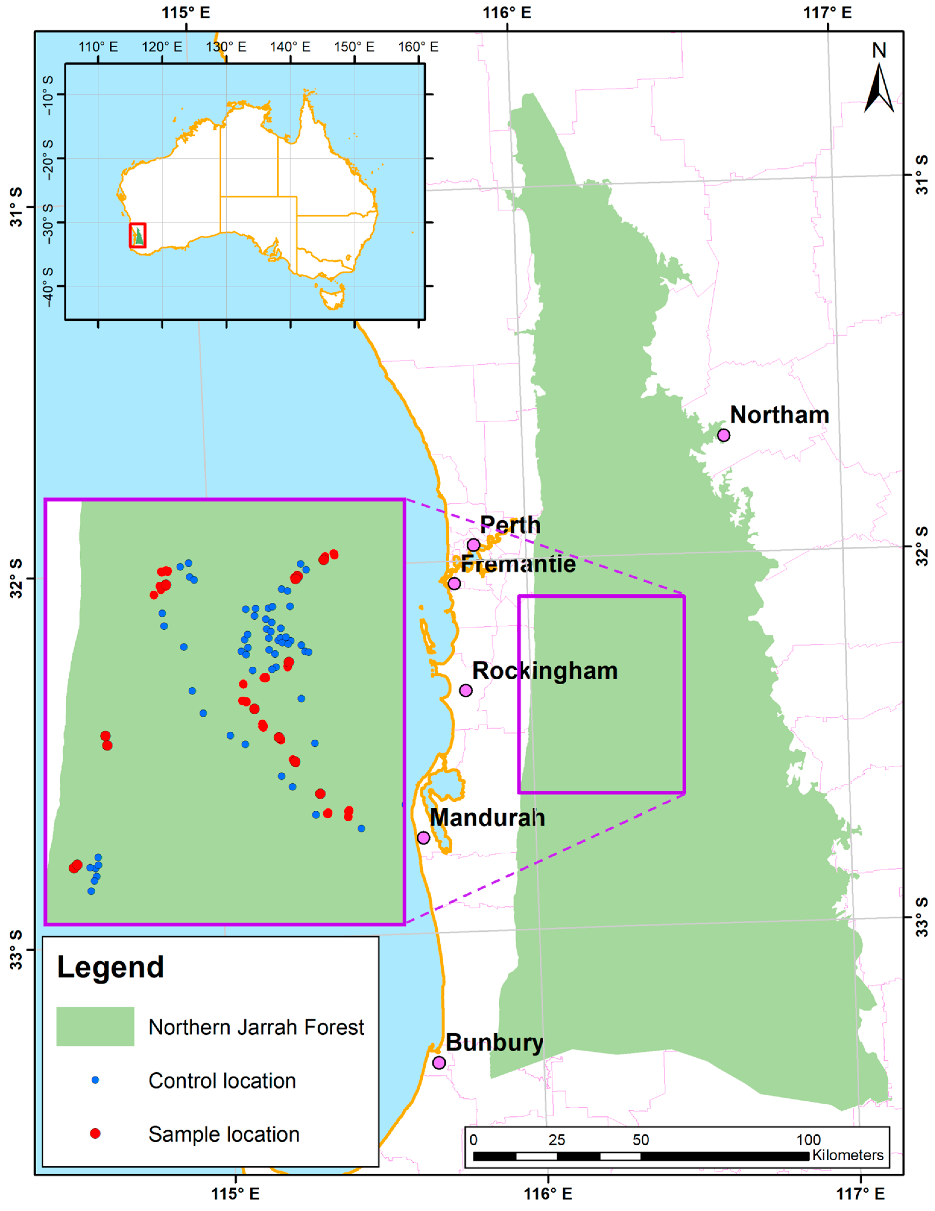
2.1. Study Area

The Northern Jarrah Forest (NJF), a broad-leaved evergreen eucalypt forest covering an area of 11,276 km2 with an average elevation of 300 m [52], is a major vegetation ecosystem in south-western Australia (Figure 2). For over 50 years, the forest has been managed for multiple purposes: timber harvesting, mining, conservation of biodiversity, catchment water protection, wildfire abatement via fuel-reduction burning, and recreation.
The NJF has a typical Mediterranean-type climate with two distinct seasons, a cool wet season and a long dry hot season that can last from 4 to 7 months [53]. The forest has a pronounced west–east rainfall gradient, with annual rainfall exceeding 1100 mm on its western edge, and diminishing to approximately 700 mm in the eastern and northern regions. The forest is dominated by jarrah (Eucalyptus marginata) which is dependent on drawing water from soil water reserves in deep regolithic soils throughout summer due to extensive root systems [16,52,54].
The study area in this paper encompasses 3000 km2 of jarrah forest (the purple frame in Figure 2) used to develop and test the ICDI remote sensing index. The chosen area contains bauxite mining sites, dams and forests with different fuel-reduction burning histories. Previous studies have reported on drought-induced canopy collapses in this forest [55,56]. Also, this area has the lowest average cloud cover compared to surrounding regions in the NJF, thereby creating optimal conditions for utilizing the greatest number of remote sensing images and yielding the most comprehensive information.

2.2. Data

We used 28 drought-affected sites (red dots Figure 2) that were defined in a study by Matusick et al. [55] with canopy damage (discolored, dead or no foliage). At those locations, damaged forest was re-delineated using Landsat images in association with Google Earth Pro. The re-delineation was based on the loss of forest canopy recorded from March to late May 2011 (see Figure 3). In this paper, we use the term “drought-affected sample” for satellite imagery analysis over the 2010–2011 dry season. These samples are polygons with areas ranging from 0.4 to 6.2 hectares.
We added 60 new control points (blue dots in Figure 2) in jarrah-dominated forest where the canopies were unaffected by drought or forest management due to their sustainable canopy condition during dry seasons. From Landsat time-series data, these forest areas had maintained NDVI values in the range 0.5–0.8 with no decline >0.05 over the past five summers (2006–2011). Control data were extracted from an area within a radius of 60 m from the control point, called the control plot. For imagery data, we used Landsat 7 ETM+ Collection 2 remote sensing images captured from October 2010 to April 2011. These images were preprocessed and converted to surface reflectance values. In this study, damaged areas were clipped to exclude bare soil and exposed rocks to concentrate on analyzing changes in the spectral reflectance of vegetation. Data from clipped polygons were compared with those from control plots to evaluate the performance of the proposed spectral index.

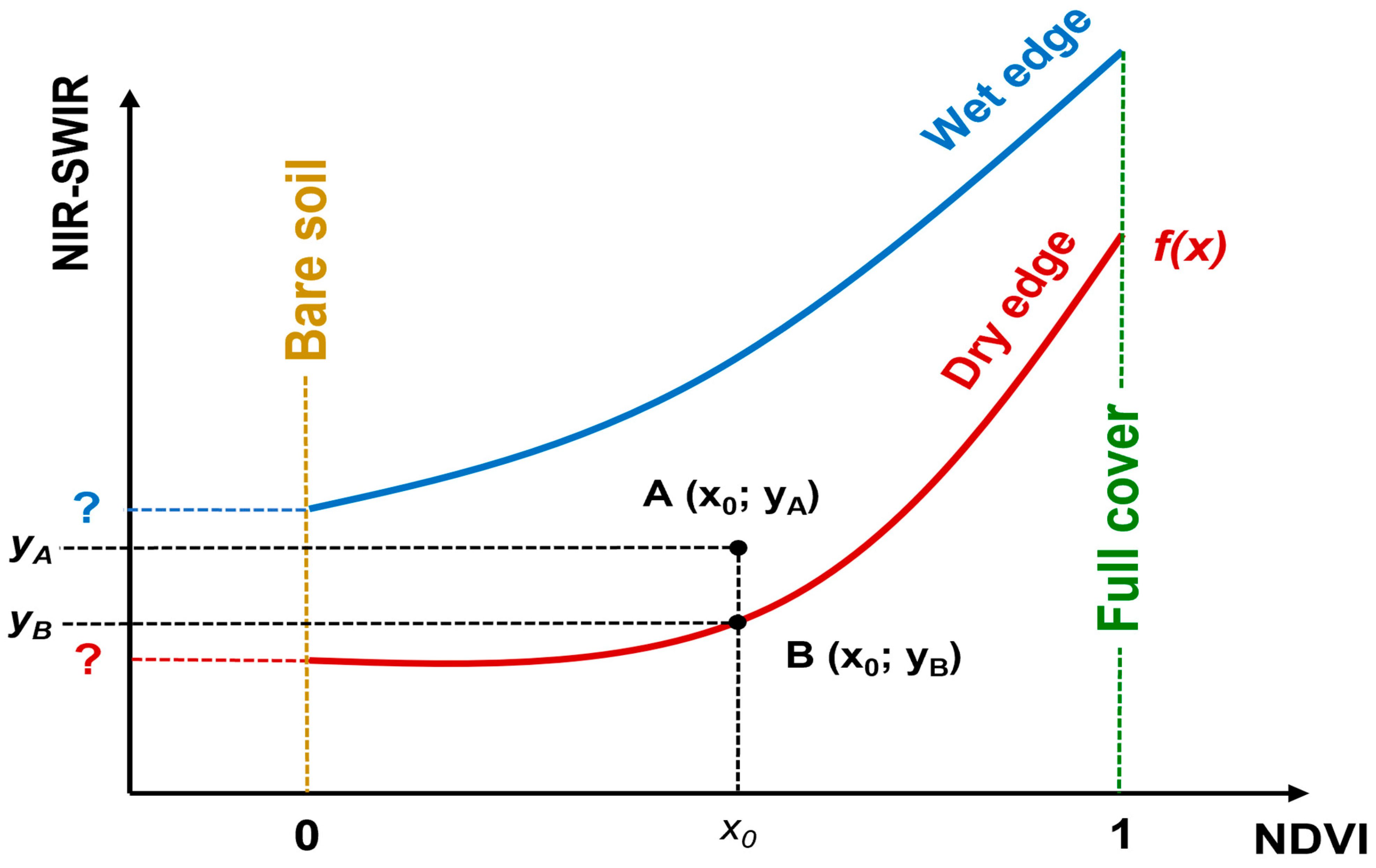
2.3. The Infrared Canopy Dryness Index (ICDI)

Inspired by the trapezoid model introduced by Sadeghi et al. [24], which employed a feature space comprising SWIR transformed reflectance (STR) and the NDVI for estimating root-zone soil moisture, we developed a similar conceptual model that illustrates the complementation between the NDVI and the NIR-SWIR index, as depicted in Figure 4. In this model, the NIR-SWIR index is calculated using the equation:
N I R S W I R i n d e x = ρ N I R     ρ S W I R ρ N I R   + ρ S W I R
where ρNIR and ρSWIR are the spectral reflectance values of NIR and SWIR, respectively.
The specific name assigned to this index varies depending on the wavelength selected in the SWIR region, in alignment with the classification system proposed by Ji et al. [43]. In this study, Landsat 7 satellite imagery data with the SWIR spectrum in band 5 (1.550–1.750 µm) was utilized for analysis. Consequently, the corresponding index employed in this context is the NDII [22,43], which is used to estimate the dynamics of water content in the vegetation canopy. Thus, the equation is:
N D I I = B 4     B 5 B 4 + B 5
where B4 and B5 are the spectral reflectance of Landsat 7 ETM+ Band 4 and Band 5, respectively. Meanwhile, the NDVI utilizes NIR and RED wavelengths to estimate fractional vegetation cover, and the index is determined as follows:
N D V I = B 4     B 3 B 4 + B 3
The dry edge f(x) can be determined by a regression analysis using samples containing the lowest values of the NDII for the corresponding NDVI bins along the x-axis. The appropriate number of bins within the NDVI range can be determined using the method proposed by Sturges [57]. According to this method, for a database containing N observations, the optimal number of bins can be calculated [57] as:
N u m b e r   o f   b i n s = 1 + 3.322 log 10 N
The study generated a 10,000-point random model within the study area on the condition that all the 10,000 points must be covered by jarrah forest. Based on remote sensing data extracted from the point cloud at two different points of time during the 2010–2011 summer, the relationship between the NDII and the NDVI at the dry edge in the study area was observed to be close to a parabola (Figure 5) instead of a linear relationship as previously used in many published studies [24,25,30].
Hence, during the method development process, we determined the dry edge using the equation:
f x = a x 2 + b x + c
In Figure 4, the deviation of observations from NIR-SWIR (i.e., the NDII at this stage) values corresponding to a particular NDVI value above this line, or distance from A to B (i.e., dAB), represents the canopy water content that exceeds the threshold of maximum water stress. With point B lying on the dry edge f(x), the corresponding NDII value can be identified as:
Y B = a X 0 2 + b X 0 + c  
Put simply, for a particular canopy condition described by NDVI = XAB, the distance AB (see Figure 4), also called dAB, increases as the canopy water content rises, thereby reflecting the observed level of canopy stress. The deviation dAB is calculated as:
d A B = Y A Y B = Y A ( a X 0 2 + b X 0 + c )  
The lower dAB, the shorter distance from the observation A to the dry edge, the higher the dryness level experienced by the canopy.
Thus, this study uses the reversed distance AB to establish a new spectral index, named Infrared Canopy Dryness Index (ICDI), which utilizes infrared spectral reflectance (NIR and SWIR) to indicate water deficiency level in the canopy. Therefore, ICDI values corresponding to the ith observation of the NDII and the NDVI are calculated as:
I C D I = ( a N D V I i 2 + b N D V I i + c ) N D I I i
where a, b and c are the parameters from the identified dry edge function.

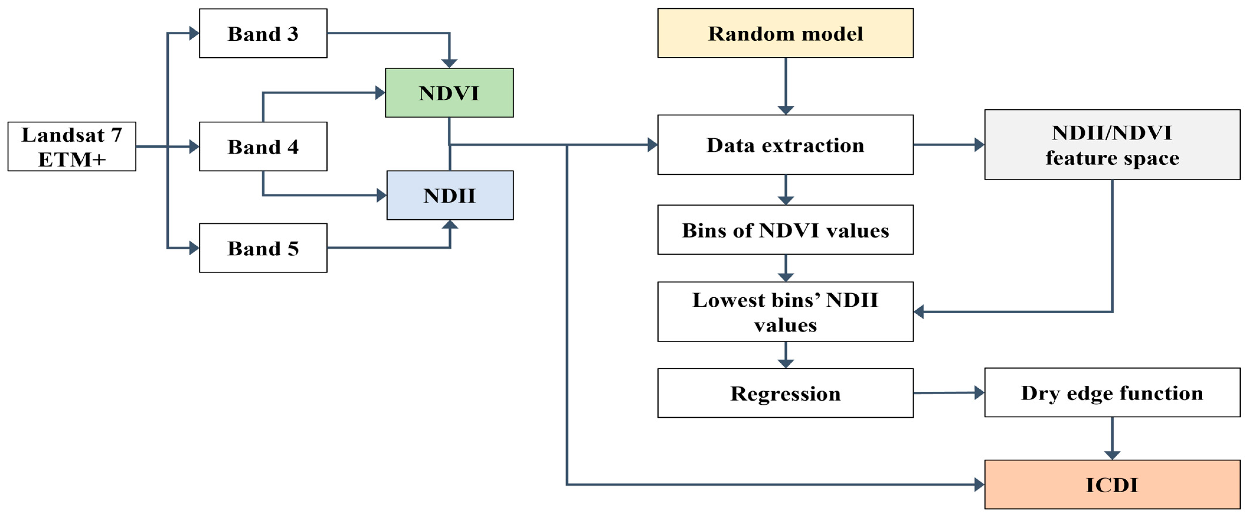
2.4. ICDI Construction and Performance Assessment

The construction of the ICDI from Landsat 7 ETM+ data is summarized in Figure 6.
Landsat 7 ETM+ was used to calculate the NDII (Equation (2)) and the NDVI (Equation (3)) over the study area. A random model including a large number of random pixels within the study area was generated using ArcGIS 10.8. Values of the NDII and the NDVI at these pixels were extracted to form a scatterplot representing the NDII/NDVI feature space. The range of NDVI values was divided into bins with the number of bins identified following Equation (4). A NDII/NDVI regression analysis was performed to identify the dry edge f(x) as in Equation (5), using the input from the pixels corresponding to the lowest NDII value from each bin. Finally, the ICDI was calculated using Equation (8).
In index performance assessment, ICDI values were extracted for the drought-affected samples and control plots monthly from October 2010 to March 2011. Any observed differences between the two datasets (i.e., stressed and non-stressed) would highlight the effectiveness of the ICDI index, particularly in instances involving drought-affected samples that exhibit smaller values. The changes over time of these values from the beginning of dry season to the event of canopy collapse can also provide valuable information for assessing the performance of the proposed index.

3. Results

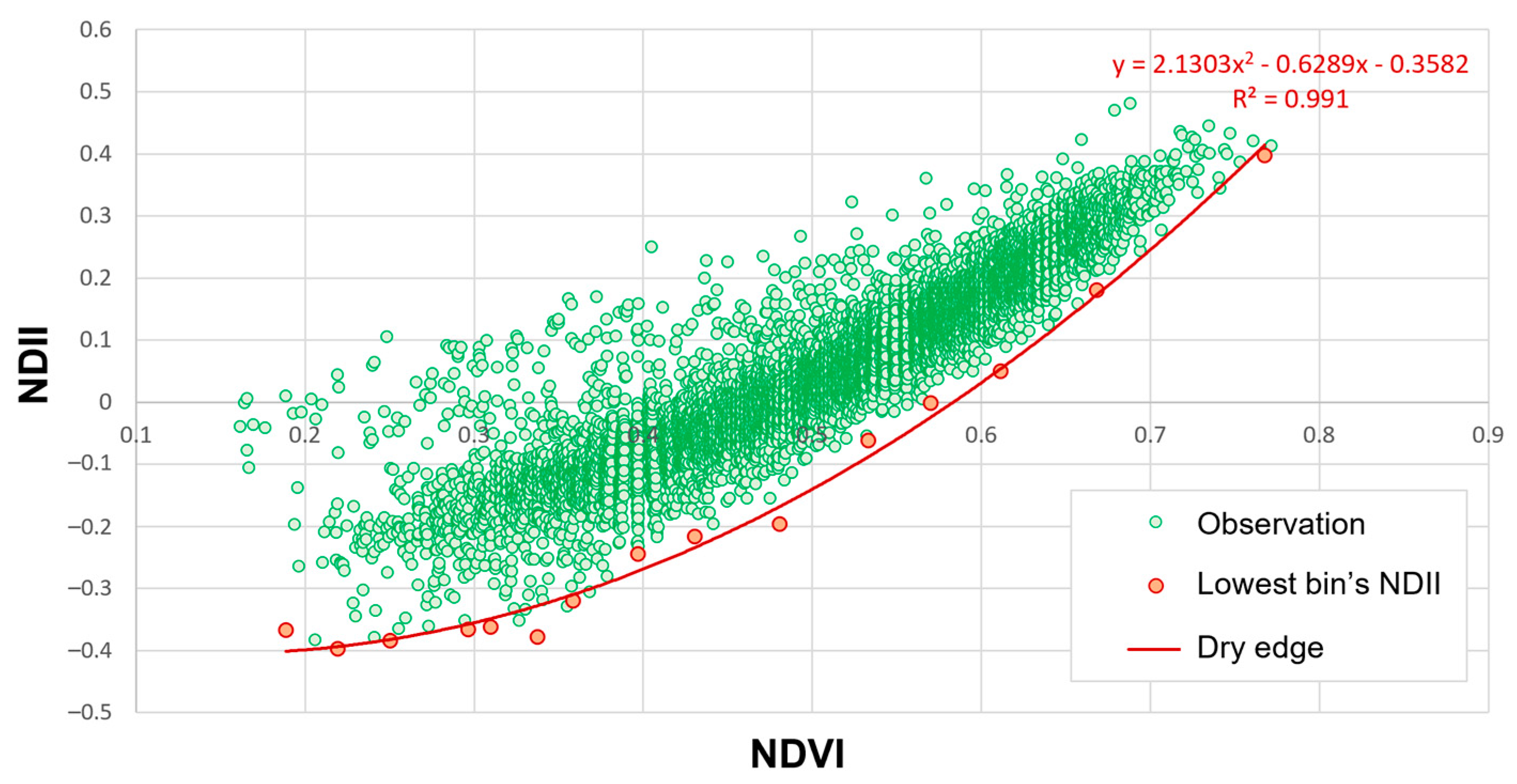
3.1. NDII/NDVI Spectral Space and ICDI Calculation

The new index was initially computed using the image captured on 14 October 2010, marking the first Landsat image available for the 2010–2011 dry season. A scatter plot mapping the NDII as a function of the NDVI was constructed using data from 10,000 random points. To ensure a comprehensive analysis, the NDVI values from these points were categorized into 15 distinct bins, employing the method outlined by Sturges [57]. Within each bin, the observation with the lowest NDII value was identified and emphasized. These highlighted points were then utilized to fit a polynomial regression, representing the dry edge, as illustrated in Figure 7.
Using the identified dry edge equation (y = 2.0163x2 − 0.515x − 0.3799), the ICDI was calculated for each pixel in the study area according to Equation (8). The resulting ICDI map (Figure 8) displays the spatial distribution of the dryness index for 14 October 2010 in the study area.
Overall, the index effectively highlights forest areas with different levels of plant dryness (Figure 8). Despite their smaller size, areas under extreme dryness are distinctly marked as orange to red on the map. Pixels displaying positive ICDI values (in dark red) indicate locations below the dry edge (see Figure 7), interspersed throughout the study area. Most of these pixels are situated in shrublands on areas with impeded subsoils that consistently exhibit significant dryness during summer (Figure 8), highlighting the index’s capability to pinpoint critical zones of water stress with precision. Figure 8 also shows that water bodies, urban regions, areas covered by clouds, and bare soil after mining bauxite had low ICDI values. This is due to the dry edge’s very low NDII values in the range of the NDVI below 0.1 (see Figure 7). Previous water stress indices, such as TVDI (Temperature Vegetation Dryness Index) and TVWSI (Temperature Vegetation Water Stress Index), typically classify bare soil as water stressed due to the absence of cooling processes from plant canopies.
An example of an ICDI output is illustrated in Figure 9. Notably, the model distinguishes between dry shrubland (i.e., hotspots) and jarrah forest undergoing recovery from fuel-reduction burning, despite these areas having similar NDVI values. Conversely, jarrah forests with dense canopy cover display relatively high ICDI values, signaling a heightened level of dryness in these regions. This observation underscores that dense forests, characterized by a high leaf area index, have a greater water demand, thereby positioning them closer to a state of stress early in the October to May dry season. This also supports the findings in the technical reports by Croton et al. [58] and Burrows et al. [17] regarding the relationship between leaf area and rainfall deficit and the benefits of thinning forests to reduce water stress.

3.2. ICDI Performance over Time

The study generated monthly ICDI maps for the summer of 2010–2011 across the study area, with data from both drought-affected samples and control plots shown in Figure 10. Throughout the summer of 2010–2011, ICDI values exhibited fluctuations for both sets of data. Prior to canopy collapse (i.e., dieback and die-off) in mid-March [55], the trend was consistent, with ICDI values from drought-affected samples consistently higher than those from the control plots. However, following the collapse event, the ICDI significantly decreased, surpassing that of the control plots. This shift suggests that the canopy became less dry post-collapse. When the overstorey had died, the still-living understorey was captured in the vegetation index and this resulted in a lower ICDI within the ecosystem.
The ICDI effectively distinguished between areas of high and low dryness; the latter in a situation where the forest was able to maintain its canopy throughout the prolonged dry summer. Additionally, Figure 10 reveals that high dryness, which indicates water stress, manifested early on, rather than in the latter half of the summer when affected canopies start dying. This indicates that the collapse events were the result of accumulated drought and heatwave conditions from the preceding months, rather than sudden onset stressors.

4. Discussion

4.1. Advantages of the ICDI and Its Application

The ICDI was developed for the early detection of water stress and prediction of future damage to forest canopies. It is important to underscore that the primary concern of the index is forested areas and their associated water deficiencies. This focus distinguishes it from other indices and how they distinguish between surface objects. Indeed, this index is influenced by the sensitivity of NIR-SWIR reflectance to vegetation cover, a factor attributable to the presence of NIR. The strength lies in its specific focus on areas covered by vegetation. As a result, the index effectively excludes bare soil areas or regions with collapsed canopy, thereby identifying areas that are experiencing the early stages of water deficit. However, numerous studies have highlighted the limitations of the NDWI and the NDII in areas with sparse vegetation cover and bare land [44,59], where NIR reflectance is relatively low. Therefore, we recommend that the ICDI is suitable for regions with extensive vegetation cover, especially forested areas.
The most effective application of the ICDI is to identify areas of significant dryness prior to or at the onset of the dry season. This early identification of areas prone to water stress will allow spatially precise and timely implementation of management measures to reduce vegetation cover, such as forest thinning and fuel-reduction burning, to help alleviate water stress. In particular, the jarrah forest is increasingly vulnerable to water stress as the water table it depends upon rapidly diminishes [60,61] under the influence of both past forest management and reduced rainfall [3]. Harvesting has been terminated, and the forests will be managed in the future for nature conservation values [17]. A legacy of previous harvesting is the regrowth of dense, often even-aged forest stands. With a reduction in rainfall, these dense stands will deplete landscape water supplies, affect streamflow and may be more prone to drought deaths. A management strategy that is being pursued is “ecological thinning”; however, this is costly to implement [17]. The ICDI provides a means of prioritizing areas for ecological thinning treatment.
In this study, we utilized Landsat 7 images, characterized by a spatial resolution of 30 × 30 m and a temporal resolution of 16 days. The quality of this imagery surpasses that of the datasets previously employed in the development of many water stress indices, such as NOAA AVRHH data (1 × 1 km) [25] and MODIS (with pixel sizes ranging from 250 m to 1000 m) [20,30,39,48]. Consequently, rather than analyzing vast areas, the ICDI enables the monitoring of forests at the scale of forest stands. This enhanced spatial resolution in depicting stressed forest features significantly aids decision-making processes, obviating the need for additional field surveys within larger forested areas such as when using low-resolution data.
Focusing on potential water-stressed tree canopies, which are prioritized for action to minimize irreversible damage, it is recommended to exclude non-forest areas using available land cover maps. Excluding areas such as water bodies, urban and mining zones will refine the value range of the ICDI, enhance the contrast of key features, and thereby reduce confusion when interpreting the results.
The results presented in Figure 8 and Figure 10 indicate that water stress manifested several months before any observable damage in the jarrah forest. The forest canopies that perished in March 2011 exhibited very low ICDI values, indicative of high stress levels, as early as October 2010, at the onset of the dry season. This indicates that a low ICDI could serve as a prognostic of potential canopy damage, should adverse conditions persist. In other words, it confirms that the death of tree canopies due to water scarcity is the culmination of cumulative effects over an extended period, highlighting the importance of early detection and intervention to mitigate long-term damage.
Examining the area surrounding the samples, as illustrated in Figure 9, it becomes evident that high canopy dryness occurs not only for trees within the sample but also extends to neighboring areas, some of which exhibit even higher dryness levels. This raises the question of why visible signs of damage are absent in areas outside the sample. There are two explanations for this phenomenon. The first is that severe and noticeable canopy damage occurs only when individual trees can no longer cope, and the adverse environmental factors exceed their tolerance threshold. These stressors and their impacts might have been present in the sample area at various times in the past, gradually diminishing the health and resilience of the plants within it, leading to the observed damage. The second explanation is that that the amount of available water stored in the regolith varies spatially, with localized areas of shallower soils and thus stored soil water.
When deploying the ICDI to analyze land cover types within the study area, distinct hotspots of dryness become readily apparent, particularly in shrubland areas. The plant species composition of these shrublands differ from the understorey in the adjacent forests. Intriguingly, these regions exhibit dryness levels significantly higher than those observed in other drought-impacted forests. This phenomenon can be attributed to the fact that many shrub species in the study area have evolved to thrive under conditions of prolonged water scarcity. This is especially true in areas with shallow soils that lack the capacity to retain water, rendering them inhospitable for the growth of trees. These shrubs remain in a desiccated state for extended periods until they receive moisture from rainfall. This perennially withered condition results in consistently low water content within these plants, leading to a spectral reflectance profile indicative of a vegetation layer under maximum water stress. Nonetheless, employing the ICDI to identify these shrubs carries substantial importance for wildfire management, as these areas become highly susceptible to ignition during the dry season.
In addition to effectively highlighting dryness hotspots in shrub areas, Figure 9 distinctly shows the contrast in ICDI values between two different states of jarrah forest, related to fire management. One area had experienced a low-intensity management fire six months prior to the imagery; in the other area a low intensity fire had occurred five years previously. The post-fire jarrah forest exhibited a noticeable reduction in canopy cover, indicated by lower NDVI values. Correspondingly, these areas demonstrated significantly lower levels of canopy dryness according to the ICDI compared to the dense jarrah forests. This observation aligns with numerous studies indicating that water stress levels are directly proportional to the leaf surface area, as represented by the Leaf Area Index (LAI) [3,16]. Indeed, a larger leaf area necessitates more water for physiological processes and cooling. Under identical soil water deficit conditions, forests with extensive leaf areas are more susceptible to rapid and severe stress. It also suggests that low intensity management fires prior to the summer drought may be a useful management technique to reduce water stress.
This understanding underscores the rationale for implementing silvicultural measures to prevent water stress in forests [16,17]. Such measures, including thinning and fuel-reduction burning, aim to reduce the leaf area of forests, thereby decreasing their water requirements and the risk and impact of water deficit. Nonetheless, the widespread application of these strategies encounters challenges related to resource allocation, time constraints and community acceptance. The ICDI emerges as a valuable predictive tool for identifying forest stands at elevated risk of water stress, allowing them to be prioritized for further intervention.

4.2. Limitations and Future Research

The primary limitation of the method in this study is the heavy reliance on accurately determining the dry edge for each survey period, which can introduce instability and inconsistency in the ICDI results across different points of time. The methodology presumes, based on the assumption of a dry edge form, that the random model encompasses a sufficiently large number of points representing all possible canopy dryness states of forest trees within the study area. However, overlooking the maximum dryness state for certain NDVI values could significantly alter the dry edge shape, thereby affecting the ICDI calculation outcomes. Alternatively, surveying all pixels within the study area to construct a comprehensive dry edge, as opposed to employing a random model, would demand excessive effort, considerable computing power, and extensive processing time. Even with such an exhaustive approach, there is no evidence to ensure that maximum dryness conditions for all forest cover levels occur in the study area. Consequently, there is a pressing need for a detailed and targeted investigation into the relationship between the NDII and the NDVI across various forest structure conditions and the corresponding water statuses. Such a study would enable a more accurate delineation of the dry edge, enhancing the reliability of the ICDI calculations.
Another limitation of the methodology employed in this study is the reliance on data from damaged forest areas for model validation. The assessment of consequential damage due to water deficit on samples currently serves as the primary basis for identifying water stress. While the impact of water deficit on forest tree canopies is evident, the severity of the damage, however, is influenced by various factors, including pests, diseases, and the overall health of the individual trees. This complexity is partially illustrated by the observation that some areas surrounding drought-affected samples exhibit lower ICDI values without clear damage to the tree canopy. Tree canopy water conditions are highly dynamic, fluctuating with time and environmental changes. An effective approach to validation might involve measuring the water content of the tree canopy at the time the imagery is captured to accurately assess dryness levels. However, such measurements would require data from ground-based spectrometers or aerial devices like drones, rather than satellite images. This underscores the need for a multi-faceted approach to validating remote sensing models, incorporating both ground-based and aerial data to provide a comprehensive understanding of canopy water stress in correspondence to spectral reflectance signals.
The ICDI is an open-ended index without a fixed value range, limiting its use to comparisons within the same geographic area and time frame. There is a critical need for enhancements that enable the ICDI to indicate relative canopy dryness levels, allowing for comparisons across different regions or over various time periods to support dynamic analyses. Future improvements could focus on leveraging features that consistently demonstrate stability over time, such as water bodies or forest areas known for optimal water conditions.

5. Conclusions

This study presents the Infrared Canopy Dryness Index (ICDI) designed to evaluate water stress within forested regions, leveraging the spectral reflectance properties of shortwave infrared channels in relation to tree canopy cover levels. We found that it could identify forest areas with incipient water stress 3–4 months prior to visible changes in canopy condition. It can be widely applied as it uses freely available satellite data. Given its efficacy, as demonstrated here, the ICDI has potential for informed decision-making in forest resource management. We propose to use the index to quantify the extent of historical forest stress in relation to past land management and rainfall distribution. However, it is necessary to undertake further validation of the ICDI in a wider range of forest systems to fully assess the efficiency of the index.

Author Contributions

Conceptualization, T.S.L., B.D. and R.H.; methodology, T.S.L. and B.D.; software, T.S.L.; writing—original draft preparation, T.S.L.; writing—review and editing, B.D. and R.H.; visualization, T.S.L.; supervision, B.D. and R.H. All authors have read and agreed to the published version of the manuscript.

Funding

T.S.L. received a Murdoch University International Postgraduate Scholarship. No additional funding was received for this study.

Data Availability Statement

The datasets presented in this article are not readily available because they are part of an ongoing study. Requests to access the datasets should be directed to the corresponding author.

Acknowledgments

The authors would like to thank Katinka Ruthrof for supplying the original data of the 2011 drought-affected sites.

Conflicts of Interest

The authors declare no conflict of interest.

References

  1. IPCC. Climate Change 2022: Impacts, Adaptation, and Vulnerability. Contribution of Working Group II to the Sixth Assessment Report of the Intergovernmental Panel on Climate Change; IPCC: Cambridge, UK; New York, NY, USA, 2022; 3056p, Available online: https://www.ipcc.ch/report/ar6/wg2/ (accessed on 15 March 2024).
  2. Cook, B.I.; Mankin, J.S.; Anchukaitis, K.J. Climate change and drought: From past to future. Curr. Clim. Change Rep. 2015, 4, 164–179. [Google Scholar] [CrossRef]
  3. Liu, N.; Harper, R.J.; Smettem, K.R.J.; Dell, B.; Liu, S. Responses of streamflow to vegetation and climate change in southwestern Australia. J. Hydrol. 2019, 572, 761–770. [Google Scholar] [CrossRef]
  4. Cholet, C.; Houle, D.; Sylvain, J.-D.; Doyon, F.; Maheu, A. Climate Change Increases the Severity and Duration of Soil Water Stress in the Temperate Forest of Eastern North America. Front. For. Glob. Change 2022, 5, 879382. [Google Scholar] [CrossRef]
  5. Wang, W.; Peng, C.; Kneeshaw, D.D.; Larocque, G.R.; Luo, Z. Drought-induced tree mortality: Ecological consequences, causes, and modeling. Environ. Rev. 2012, 20, 109–121. [Google Scholar] [CrossRef]
  6. Allen, C.D.; Breshears, D.D.; McDowell, N.G. On underestimation of global vulnerability to tree mortality and forest die-off from hotter drought in the anthropocene. Ecosphere 2015, 6, 1–55. [Google Scholar] [CrossRef]
  7. Bradford, J.B.; Shriver, R.K.; Robles, M.D.; McCauley, L.A.; Woolley, T.J.; Andrews, C.A.; Crimmins, M.; Bell, D.M. Tree mortality response to drought-density interactions suggests opportunities to enhance drought resistance. J. Appl. Ecol. 2022, 59, 549–559. [Google Scholar] [CrossRef]
  8. Trenberth, K.E.; Dai, A.; Van Der Schrier, G.; Jones, P.D.; Barichivich, J.; Briffa, K.R.; Sheffield, J. Global warming and changes in drought. Nat. Clim. Change 2014, 4, 17–22. [Google Scholar] [CrossRef]
  9. Le, T.S.; Harper, R.; Dell, B. Application of Remote Sensing in Detecting and Monitoring Water Stress in Forests. Remote Sens. 2023, 15, 3360. [Google Scholar] [CrossRef]
  10. Xu, P.; Zhou, T.; Yi, C.; Luo, H.; Zhao, X.; Fang, W.; Gao, S.; Liu, X. Impacts of Water Stress on Forest Recovery and Its Interaction with Canopy Height. Int. J. Environ. Res. Public Health 2018, 15, 1257. [Google Scholar] [CrossRef]
  11. Imadi, S.R.; Gul, A.; Dikilitas, M.; Karakas, S.; Sharma, I.; Ahmad, P. Water stress: Types, causes, and impact on plant growth and development. In Water Stress and Crop Plants: A Sustainable Approach; Ahmad, P., Ed.; John Wiley & Sons Ltd.: Hoboken, NJ, USA, 2016; Volume 2. [Google Scholar]
  12. Liu, N.; Deng, Z.; Wang, H.; Luo, Z.; Gutiérrez-Juradob, H.A.; He, X.; Guan, H. Thermal remote sensing of plant water stress in natural ecosystems. For. Ecol. Manag. 2020, 476, 118433. [Google Scholar] [CrossRef]
  13. Laskari, M.; Menexes, G.; Kalfas, I.; Gatzolis, I.; Dordas, C. Water Stress Effects on the Morphological, Physiological Characteristics of Maize (Zea mays L.), and on Environmental Cost. Agronomy 2022, 12, 2386. [Google Scholar] [CrossRef]
  14. Sohn, J.A.; Saha, S.; Bauhus, J. Potential of forest thinning to mitigate drought stress: A metaanalysis. For. Ecol. Manag. 2016, 380, 261–273. [Google Scholar] [CrossRef]
  15. Gavinet, J.; Ourcival, J.M.; Gauzere, J.; De Jalón, L.G.; Limousin, J.M. Drought mitigation by thinning; Benefits from the stem to the stand along 15 years of experimental rainfall exclusion in a holm oak coppice. For. Ecol. Manag. 2020, 473, 118266. [Google Scholar] [CrossRef]
  16. Harper, R.; Smettem, K.R.J.; Ruprecht, J.K.; Dell, B.; Liu, N. Forest-water interactions in the changing environment of south-western Australia. Ann. For. Sci. 2019, 76, 95. [Google Scholar] [CrossRef]
  17. Burrows, N.; Baker, P.; Harper, R.; Silberstein, R. A Report on Silvicultural Guidelines 2033 Forest Management Plan for the Western Australian; Department of Biodiversity, Conservation and Attractions: 2022. Available online: https://www.dbca.wa.gov.au/sites/default/files/2022-10/Independent%20Silviculture%20Review%20Panel%20Report%20May%202022.pdf (accessed on 15 March 2024).
  18. Ceccato, P.; Flasse, S.; Tarantola, S.; Jacquemoud, S.; Grégoire, J.-M. Detecting vegetation leaf water content using reflectance in the optical domain. Remote Sens. Environ. 2001, 77, 22–33. [Google Scholar] [CrossRef]
  19. Maki, M.; Ishiahra, M.; Tamura, M. Estimation of leaf water status to monitor the risk of forest fires by using remotely sensed data. Remote Sens. Environ. 2004, 90, 441–450. [Google Scholar] [CrossRef]
  20. Fensholt, R.; Sandholt, I. Derivation of a shortwave infrared water stress index from MODIS near- and shortwave infrared data in a semiarid environment. Remote Sens. Environ. 2003, 87, 111–121. [Google Scholar] [CrossRef]
  21. Hunt, E.R.; Rock, B.N.; Nobel, P.S. Measurement of leaf relative water content by infrared reflectance. Remote Sens. Environ. 1987, 22, 429–435. [Google Scholar] [CrossRef]
  22. Hunt, E.R.; Rock, B.N. Detection of changes in leaf water content using Near- and Middle-Infrared reflectances. Remote Sens. Environ. 1989, 30, 43–54. [Google Scholar] [CrossRef]
  23. Gao, B.-c. A normalized difference water index for remote sensing of vegetation liquid water from space—NDWI. Remote Sens. Environ. 1996, 58, 257–266. [Google Scholar] [CrossRef]
  24. Sadeghi, M.; Babaeian, E.; Tuller, M.; Jones, S.B. The optical trapezoid model: A novel approach to remote sensing of soil moisture applied to Sentinel-2 and Landsat-8 observations. Remote Sens. Environ. 2017, 198, 52–68. [Google Scholar] [CrossRef]
  25. Sandholt, I.; Rasmussen, K.; Andersen, J. A simple interpretation of the surface temperature/vegetation index space for assessment of surface moisture status. Remote Sens. Environ. 2002, 79, 213–224. [Google Scholar] [CrossRef]
  26. Jang, J.D.; Viau, A.A.; Anctil, F. Thermal-water stress index from satellite images. Int. J. Remote Sens. 2006, 27, 1619–1639. [Google Scholar] [CrossRef]
  27. Carlson, T.N.; Gillies, R.R.; Perry, E.M. A method to make use of thermal infrared temperature and NDVI measurements to infer surface soil water content and fractional vegetation cover. Remote Sens. Rev. 1994, 52, 45–59. [Google Scholar] [CrossRef]
  28. Jackson, R.D.; Idso, S.B.; Reginato, R.J.; Pinter, P.J. Canopy temperature as a crop water stress indicator. Water Resour. Res. 1981, 17, 1133–1138. [Google Scholar] [CrossRef]
  29. Amani, M.; Salehi, B.; Mahdavi, S.; Masjedi, A.; Dehnavi, S. Temperature-Vegetation-soil Moisture Dryness Index (TVMDI). Remote Sens. Environ. 2017, 197, 1–14. [Google Scholar] [CrossRef]
  30. Joshi, R.C.; Ryu, D.; Sheridan, G.J.; Lane, P.N.J. Modeling Vegetation Water Stress over the Forest from Space: Temperature Vegetation Water Stress Index (TVWSI). Remote Sens. 2021, 13, 4635. [Google Scholar] [CrossRef]
  31. Cheng, T.; Riaño, D.; Koltunov, A.; Whiting, M.L.; Ustin, S.L.; Rodriguez, J. Detection of diurnal variation in orchard canopy water content using MODIS/ASTER airborne simulator (MASTER) data. Remote Sens. Environ. 2013, 132, 1–12. [Google Scholar] [CrossRef]
  32. Hsiao, T.C. Plant Responses to Water Stress. Annu. Rev. Plant Physiol. 1973, 24, 519–570. [Google Scholar] [CrossRef]
  33. Pirzad, A.; Shakiba, M.R.; Zehtab-Salmasi, S.; Mohammadi, S.A.; Darvishzadeh, R.; Samadi, A. Effect of water stress on leaf relative water content, chlorophyll, proline and soluble carbohydrates in Matricaria chamomilla L. J. Med. Plants Res. 2011, 5, 2483–2488. [Google Scholar]
  34. Lisar, S.Y.S.; Motafakkerazad1, R.; Hossain, M.M.; Rahman, I.M.M. Water Stress in Plants: Causes, Effects and Responses. In Water Stress; Rahman, I.M.M., Hasegawa, H., Eds.; IntechOpen: London, UK, 2012. [Google Scholar]
  35. Zhang, F.; Zhou, G. Estimation of vegetation water content using hyperspectral vegetation indices: A comparison of crop water indicators in response to water stress treatments for summer maize. BMC Ecol. 2019, 19, 18. [Google Scholar] [CrossRef]
  36. Hardisky, M.A.; Klemas, V.; Smart, R.M. The Influence of Soil Salinity, Growth Form, and Leaf Moisture on the Spectral Radiance of Spartina alterniflora Canopies. Photogramm. Eng. Remote Sens. 1983, 49, 77–83. [Google Scholar]
  37. Kimes, D.S.; Markham, B.L.; Tucker, C.J.; McMurtrey, J.E. Temporal relationships between spectral response and agronomic variables of a corn canopy. Remote Sens. Environ. 1981, 11, 401–411. [Google Scholar] [CrossRef]
  38. Carlson, T.N.; Ripley, D.A. On the relation between NDVI, fractional vegetation cover, and leaf area index. Remote Sens. Environ. 1997, 62, 241–252. [Google Scholar] [CrossRef]
  39. Wan, Z.; Wang, P.; Li, X. Using MODIS Land Surface Temperature and Normalized Difference Vegetation Index products for monitoring drought in the southern Great Plains, USA. Int. J. Remote Sens. 2004, 25, 61–72. [Google Scholar] [CrossRef]
  40. Tucker, C.J. Remote sensing of leaf water content in the near infrared. Remote Sens. Environ. 1980, 10, 23–32. [Google Scholar] [CrossRef]
  41. Wu, C.; Niu, Z.; Tang, Q.; Huang, W. Predicting vegetation water content in wheat using normalized difference water indices derived from ground measurements. J. Plant Res. 2009, 122, 317–326. [Google Scholar] [CrossRef] [PubMed]
  42. Gausman, H.W. Reflectance of leaf components. Remote Sens. Environ. 1977, 6, 1–9. [Google Scholar] [CrossRef]
  43. Ji, L.; Zhang, L.; Wylie, B.K.; Rover, J. On the terminology of the spectral vegetation index (NIR − SWIR)/(NIR + SWIR). Int. J. Remote Sens. 2011, 32, 6901–6909. [Google Scholar] [CrossRef]
  44. Quemada, C.; Pérez-Escudero, J.M.; Gonzalo, R.; Ederra, I.; Santesteban, L.G.; Torres, N.; Iriarte, J.C. Remote sensing for plant water content monitoring: A review. Remote Sens. 2021, 12, 2088. [Google Scholar] [CrossRef]
  45. Li, C.; Czyż, E.A.; Halitschke, R.; Baldwin, I.T.; Schaepman, M.E.; Schuman, M.C. Evaluating potential of leaf reflectance spectra to monitor plant genetic variation. Plant Methods 2023, 19, 108. [Google Scholar] [CrossRef]
  46. Ge, Y.; Atefi, A.; Zhang, H.; Miao, C.; Ramamurthy, R.K.; Sigmon, B.; Yang, J.; Schnable, J.C. High-throughput analysis of leaf physiological and chemical traits with VIS–NIR–SWIR spectroscopy: A case study with a maize diversity panel. Plant Methods 2019, 15, 66. [Google Scholar] [CrossRef] [PubMed]
  47. Ghulam, A.; Li, Z.L.; Qin, Q.; Yimit, H.; Wang, J. Estimating crop water stress with ETM+ NIR and SWIR data. Agric. For. Meteorol. 2008, 148, 1679–1695. [Google Scholar] [CrossRef]
  48. Holzman, M.E.; Rivas, R.E.; Bayala, M.I. Relationship between TIR and NIR-SWIR as Indicator of Vegetation Water Availability. Remote Sens. 2021, 13, 3371. [Google Scholar] [CrossRef]
  49. Key, C.H.; Benson, N.C. Landscape assessment: Remote sensingof severity, the normalized burn ratio; and ground measure of severity, the composite burn index. In FIREMON: Fire Effects Monitoring and Inventory System; Lutes, D.C., Keane, R.E., Caratti, J.F., Key, C.H., Benson, N.C., Gangi, L.J., Eds.; USDA Forest Service, Rocky Mountain: Lakewood, CO, USA, 2005. [Google Scholar]
  50. Yilmaz, M.T.; Hunt, E.R.; Goins, L.D.; Ustin, S.L.; Vanderbilt, V.C.; Jackson, T.J. Vegetation water content during SMEX04 from ground data and landsat 5 thematic mapper imagery. Remote Sens. Environ. 2008, 112, 350–362. [Google Scholar] [CrossRef]
  51. Zhou, H.; Zhou, G.; Song, X.; He, Q. Dynamic Characteristics of Canopy and Vegetation Water Content during an Entire Maize Growing Season in Relation to Spectral-Based Indices. Remote Sens. 2022, 14, 584. [Google Scholar] [CrossRef]
  52. Dell, B.; Havel, J.J. The jarrah forest, an introduction. In The Jarrah Forest, A Complex Mediterranean Ecosystem; Dell, B., Havel, J.J., Malajczuk, N., Eds.; Kluwer Academic Publisher: Dordrecht, The Netherlands, 1989. [Google Scholar]
  53. Gentilli, J. Climate of the jarrah forest. In The Jarrah Forest, A Complex Mediterranean Ecosystem; Dell, B., Havel, J.J., Malajczuk, N., Eds.; Kluwer Academic Publisher: Dordrecht, The Netherlands, 1989. [Google Scholar]
  54. Szota, C.; Veneklaas, E.J.; Koch, J.M.; Lambers, H. Root Architecture of Jarrah (Eucalyptus marginata) Trees in Relation to Post-Mining Deep Ripping in Western Australia. Restor. Ecol. 2007, 15, s65–s73. [Google Scholar] [CrossRef]
  55. Matusick, G.; Ruthrof, K.X.; Brouwers, N.C.; Dell, B.; Hardy, G.S.J. Sudden forest canopy collapse corresponding with extreme drought and heat in a mediterranean-type eucalypt forest in southwestern Australia. Eur. J. For. Res. 2013, 132, 497–510. [Google Scholar] [CrossRef]
  56. Matusick, G.; Ruthrof, K.X.; Kala, J.; Brouwers, N.C.; Breshears, D.D.; Hardy, G. Chronic historical drought legacy exacerbates tree mortality and crown dieback during acute heatwave-compounded drought. Environ. Res. Lett. 2018, 13, 095002. [Google Scholar] [CrossRef]
  57. Sturges, H.A. The Choice of a Class Interval. J. Am. Stat. Assoc. 1926, 21, 65–66. [Google Scholar] [CrossRef]
  58. Croton, J.T.; Dalton, G.T.; Green, K.A.; Mauger, G.W.; Dalton, J.A. Northern Jarrah Forest Water-Balance Study to Inform the Review of Silviculture Guidelines; Forest and Ecosystem Management Division, Technical Report No. 9; Department of Parks and Wildlife, Western Australia: Perth, Australia, 2014. Available online: https://www.dbca.wa.gov.au/media/2183/download (accessed on 15 March 2024).
  59. Hunt, E.R.; Ustin, S.L.; Riano, D. Remote Sensing of Leaf, Canopy, and Vegetation Water Contents for Satellite Environmental Data Records. In Satellite-Based Applications on Climate Change; Qu, J., Powell, A., Sivakumar, M.V.K., Eds.; Springer: Berlin/Heidelberg, Germany, 2013; pp. 335–357. [Google Scholar]
  60. Smettem, K.R.J.; Waring, R.J.; Callow, J.; Wilson, M.; Mu, Q. Satellite-derived estimates of forest leaf area index in south-west Western Australia are not tightly coupled to inter-annual variations in rainfall: Implications for groundwater decline in a drying climate. Glob. Change Biol. 2013, 19, 2401–2412. [Google Scholar] [CrossRef] [PubMed]
  61. Kinal, J.; Stoneman, G.L. Disconnection of groundwater from surface water causes a fundamental change in hydrology in a forested catchment in south-western Australia. J. Hydrol. 2012, 472–473, 14–24. [Google Scholar] [CrossRef]
Figure 1. Relationship between canopy cover and water content in response to canopy dryness (original by Thai Son Le).
Forests 15 00915 g001
Figure 2. Map of the Northern Jarrah Forest showing the study area (purple frame) with sample (drought-affected) and control (healthy forest) locations.
Forests 15 00915 g002
Figure 3. Example of a drought-affected sample at location (X: 429525; Y: −3583515) on 14 October 2010 (A) and 23 March 2011 (B) (source: Google Earth Pro). This is during the dry, summer period.
Forests 15 00915 g003
Figure 4. General conceptual model of the NIR-SWIR/NDVI feature space (original by Thai Son Le).
Forests 15 00915 g004
Figure 5. The dry edge from a 10,000-point random model at two different times for the study area.
Forests 15 00915 g005
Figure 6. Flowchart illustrating the construction of the ICDI.
Forests 15 00915 g006
Figure 7. Dry edge identification in the NDII/NDVI feature space (14 October 2010).
Forests 15 00915 g007
Figure 8. Example of an ICDI map for the study area (see Figure 2 for location) from the Landsat 7 image captured on 14 October 2010 (lower values indicate higher stress).
Forests 15 00915 g008
Figure 9. Example of ICDI output delineating different dryness values according to a range of contributory factors (14 October 2010).
Forests 15 00915 g009
Figure 10. The change over time of the ICDI index from drought-affected samples and control plots during 2010–2011 dry season. Note that in March 2011 the canopies were dead in the drought-affected sites and their ICDI was lower than for the healthy control plots.
Forests 15 00915 g010
Disclaimer/Publisher’s Note: The statements, opinions and data contained in all publications are solely those of the individual author(s) and contributor(s) and not of MDPI and/or the editor(s). MDPI and/or the editor(s) disclaim responsibility for any injury to people or property resulting from any ideas, methods, instructions or products referred to in the content.

