Coupling the PROSAIL Model and Machine Learning Approach for Canopy Parameter Estimation of Moso Bamboo Forests from UAV Hyperspectral Data

Abstract

Parameters such as the leaf area index (LAI), canopy chlorophyll content (CCH), and canopy carotenoid content (CCA) are important indicators for evaluating the ecological functions of forests. Currently, rapidly developing unmanned aerial vehicles (UAV) equipped with hyperspectral technology provide advanced technical means for the real-time dynamic acquisition of regional vegetation canopy parameters. In this study, a hyperspectral sensor mounted on a UAV was used to acquire the data in the study area, and the canopy parameter estimation model of moso bamboo forests (MBF) was developed by combining the PROSAIL radiative transfer model and the machine learning regression algorithm (MLRA), inverted the canopy parameters such as LAI, CCH, and CCA. The method first utilized the extended Fourier amplitude sensitivity test (EFAST) method to optimize the global sensitivity analysis and parameters of the PROSAIL model, and the successive projections algorithm (SPA) was used to screen the characteristic wavebands for the inversion of MBF canopy parameter inversion. Then, the optimized PROSAIL model was used to construct the ‘LAI-CCH-CCA-canopy reflectance’ simulation dataset for the MBF; multilayer perceptron regressor (MLPR), extra tree regressor (ETR), and extreme gradient boosting regressor (XGBR) employed used to construct PROSAIL_MLPR, PROSAIL_ETR, and PROSAIL_XGBR, respectively, as the three hybrid models. Finally, the best hybrid model was selected and used to invert the spatial distribution of the MBF canopy parameters. The following results were obtained: Waveband sensitivity analysis reveals 400–490 and 710–1000 nm as critical for LAI, 540–650 nm for chlorophyll, and 490–540 nm for carotenoids. SPA narrows down the feature bands to 43 for LAI, 19 for CCH, and 9 for CCA. The three constructed hybrid models were able to achieve high-precision inversion of the three parameters of the MBF, the model fitting accuracy of PROSAIL_MLRA reached more than 95%, with lower RMSE values, and the PROSAIL_XGBR model yielded the best fitting results. Our study provides a novel method for the inversion of forest canopy parameters based on UAV hyperspectral data.

1. Introduction

The leaf area index (LAI), canopy chlorophyll content (CCH), and canopy carotenoid content (CCA) are crucial parameters of a canopy. They play a significant role in the transmission of material energy and solar radiation within forest ecosystems. Furthermore, they help maintain the spatial distribution of environmental factors and physiological parameters. As such, these parameters have emerged as important indicators of regional and even global ecological and environmental changes [1,2,3,4]. LAI and CCH are crucial parameters for studying biophysical processes such as forest carbon–water cycles, the photosynthetic rate, the transpiration rate, and precipitation interception [5,6,7]. CCH and CCA are crucial photosynthetic pigments that not only absorb, transfer, and convert light energy but also protect the photosystem when there is an excess of light energy [8]. Therefore, the accurate estimation of LAI, CCH, and CCA is vital for assessing tree growth and the carbon sequestration function of forest ecosystems [9,10].

Remote sensing, due to its real-time, dynamic, and non-destructive nature, provides an opportunity to monitor spatial and temporal changes in forest canopy parameters over large areas [11,12]. It is of great significance to establish an efficient monitoring system. Advances in remote sensing technology have expanded from multispectral to hyperspectral fields, greatly facilitating accurate assessment and research on forest LAI and canopy pigmentation [13]. However, their low robustness and susceptibility to saturation limit the further application of these methods.

Unlike multispectral data, hyperspectral data offer full-band radiometric information. This provides a comprehensive characterization of features related to canopy structure, as well as biochemical and physiological characteristics [14,15,16]. However, challenges such as data redundancy and band autocorrelation can lead to unnecessary computational resource usage. These issues also present challenges in achieving large-scale remote sensing parameter inversion applications. Therefore, the extraction of the sensitive characteristic bands from hyperspectral data plays an important role in the estimation of forest LAI, CCH, and CCA. Previous studies have established relationships between forest canopy parameters and sensitive band reflectance, vegetation indices, or spectral transformation values based on specific conditions [17,18]. While these methods are relatively simple and easy to use, they have their limitations. The empirical relationship between the two is influenced by external factors such as the sensor, vegetation type, and background reflectance. This influence is not effectively represented, leading to a lack of generalization. As a result, the selected feature spectra for LAI and CAB monitoring may not be applicable in different environments and conditions [19,20]. It is essential to identify sensitive spectral features from hyperspectral datasets for optimal extraction of LAI, CCH, and CCA in forest environments.

The radiative transfer model is capable of demonstrating the physical mechanisms of absorption, bidirectional reflection, and the transmission of solar radiation within the forest canopy. It can analyze the interactions between electromagnetic waves and canopy parameters. This allows it to simulate the canopy reflectance for various vegetation types with high precision, using measurements of leaf reflectance and other related physicochemical parameters. Consequently, the simulation of canopy reflectance based on the radiative transfer model and its applications has become a burgeoning field of research in recent years [21,22,23]. However, the model structure is complex, and the physicochemical parameters of vegetation, canopy structure, and observation geometry can cause changes in the reflectance spectra of vegetation [24]; these changes result in incomplete independence of the model parameters, and the coupling effect between the parameters will also have an impact on the simulation results of the leaf optical PROSPECT + canopy scale (SAIL) PROSAIL model. Therefore, quantitatively or qualitatively analyzing the degree of sensitivity of the model parameters to different bands is an important prerequisite for extracting sensitive spectral features of optimal forest canopy parameters [25,26]. The successive projections algorithm (SPA) adeptly identifies a subset of wavelengths with reduced collinearity through an elementary projection operation within the vector space framework. Additionally, it efficiently mitigates variable collinearity, minimizes data overlap, and augments the accuracy of predictive modeling [27,28]. Therefore, the leaf optical PROSAIL model coupled with the SPA can be used to simulate the hyperspectral dataset of the forest canopy parameters and select the most sensitive spectral features.

Building inversion models for forest canopy parameters based on selected sensitive spectral features is a key technique in remote sensing. Hybrid models blend the adaptability of statistical models with the theoretical grounding of physical models. They can adapt to complex data patterns while maintaining the interpretability of physical processes. The models can address issues commonly associated with statistical models, such as data redundancy, overfitting, and underfitting. Moreover, they are adept at handling uncertainty and noise, thereby enhancing the accuracy and stability of parameter estimation [29,30,31,32,33]. Machine learning regression algorithms (MLRA) have a strong ability to mine and learn empirical relationships and can mine useful information and establish learned empirical relationships from a large number of remote sensing feature variables and parameters [34,35,36,37,38]. MLRA, such as Artificial Neural Networks and Support Vector Machine Regression, have been widely used in parameter estimation, but for high-dimensional data, the training speed is slow and prone to overfitting problems. While Multilayer Perceptron Regression (MLPR), Extreme Random Tree Regression (ETR), and XGBoost Regression (XGBR) can better deal with the nonlinear problem, XGBR can automatically deal with the missing values and provide the model with higher prediction accuracy [39,40].

Moso bamboo forests (MBF) are integral to China’s subtropical ecosystems, contributing significantly to carbon sequestration and, thus, to the mitigation of global climate change, as well as the regulation of carbon balances on regional and global levels [41,42]. Distinct from other forests, MBF has demonstrated unique biennial phenological phenomena: the sprouting and growth of bamboo culms in the on-years, contrasted with the senescence and abscission of foliage in the off-years [43,44]. Therefore, the accurate monitoring of the canopy parameters is important for modeling the carbon cycle in bamboo forest ecosystems. In this study, MBF was used as the research object, hyperspectral remote sensing data of the MBF in the study area were acquired by a UAV-mounted hyperspectral sensor, a canopy parameter estimation model of the MBF was constructed with the PROSAIL radiative transfer model combined with the MLRA, and canopy parameters, such as LAI, CCH, and CCA, were inverted. The method first utilized the EFAST method to optimize the global sensitivity analysis and parameters of the PROSAIL model, and the SPA was utilized to identify the characteristic wavebands of MBF canopy parameter inversion. Then, the optimized PROSAIL model was used to construct the ‘LAI-CCH-CCA-canopy reflectance’ simulation dataset for the MBF; MLPR, ETR, and XGBR were employed to construct PROSAIL_MLPR, PROSAIL_ETR, and PROSAIL_XGBR, respectively, as the three hybrid models. Finally, the best hybrid model was selected and used to invert the spatial distribution of the MBF canopy parameters. Our study provides a new method for the inversion of the forest canopy parameters based on UAV hyperspectral data.

2. Materials and Methods

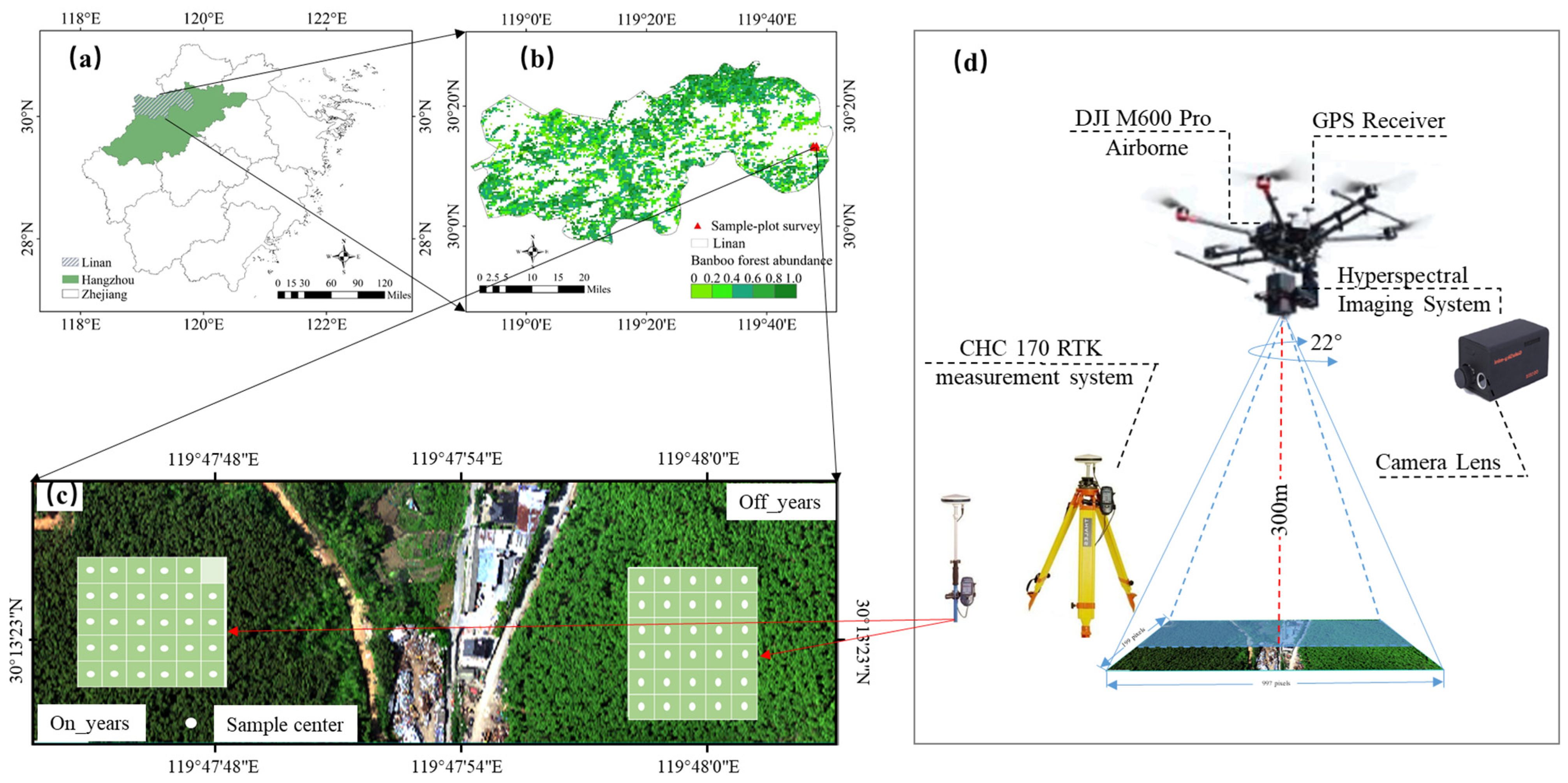
2.1. Experimental Site

The study site is located in Lin’an District, Hangzhou (30°13′09″–30°13′27″ N, 119°47′43″–119°48′11″ E). It has a subtropical monsoon climate that is warm and humid, with sufficient light, abundant rainfall, and four distinct seasons. The average annual temperature is 16.4 °C, the frost-free period is 237 days, the sunshine time is 1847.3 h, and the annual precipitation is 1613.9 mm. The territory is mainly hilly and mountainous, with terrain tilting from northwest to southeast, and the three-dimensional climate is evident. The field survey was conducted on 2 May 2023, and two phenological phenomena were selected for the study in both on-years and off-years in the sample plots. Within each kind of phenology, areas with gentle terrain slopes, uniform distribution of vegetation, and small variations were selected for the measurement, and the size of the sample squares was 10 m × 10 m, with a total of 59 sample squares (29 in on-years and 30 in off-years), on-years missing one due to topography. The distribution is shown in Figure 1.

2.2. Data Collection and Organization

2.2.1. Sample Plot Data Collection and Measurement

The ground measurement data generally represented the vegetation changes in the study area while minimizing the field measurement effort. Canopy photographs of each sample site were collected with a digital camera with a fisheye lens, and LAI was calculated for each sample site using a WinSCANOPY2009a (WinSCANOPY2009a; Regent Instruments, SteFoy, QC, Canada) canopy analyzer. Sample leaves from two to three branches were simultaneously collected from the top of the canopy in the mature sun-exposed portion using tall pruning shears [45]. The relative chlorophyll content index was immediately measured using a chlorophyll content meter and converted to absolute CAB using a correlation equation. To measure CAR, a random subset of 20 samples from 59 was rapidly transferred to an ice-filled cooler to prevent moisture loss. Upon collection, 0.1 g of fresh leaf from each sample was weighed, and leaf area (S) was measured using graph paper. Leaves were then cut, placed in 10 mL tubes, and immersed in 10 mL hybrid extraction solution composed of anhydrous ethanol, acetone, and distilled water at a ratio of 45:45:10. The tubes were sealed and stored in darkness at room temperature for 24 h until leaves tissue whitened. Thereafter, the CAR extract was decanted into 1 cm pathlength cuvettes, and absorbances at 470 nm, 645 nm, and 663 nm were measured against the extraction blank.

CCH and CCA are calculated from Equations (1)–(4).

$$CAB \left(\mathsf{\mu }\mathrm{g}/{\mathrm{c}\mathrm{m}}^2\right)=0.002\times CCI \left(\mathsf{\mu }\mathrm{g}/{\mathrm{c}\mathrm{m}}^2\right)+0.013$$

(1)

$$\mathrm{C}\mathrm{C}\mathrm{H} \left(\mathsf{\mu }\mathrm{g}/{\mathrm{c}\mathrm{m}}^2\right)=\mathrm{C}\mathrm{A}\mathrm{B} \left(\mathsf{\mu }\mathrm{g}/{\mathrm{c}\mathrm{m}}^2\right)\times \mathrm{L}\mathrm{A}\mathrm{I}$$

(2)

$$\mathrm{C}\mathrm{A}\mathrm{R} \left(\mathsf{\mu }\mathrm{g}/{\mathrm{c}\mathrm{m}}^2\right)=0.025\times (1000\times {∆\mathrm{A}}_{470}-2851.304\times {∆\mathrm{A}}_{649}+811.7385\times {∆\mathrm{A}}_{665})/245S$$

(3)

$$\mathrm{C}\mathrm{C}\mathrm{A} \left(\mathsf{\mu }\mathrm{g}/{\mathrm{c}\mathrm{m}}^2\right)=\mathrm{C}\mathrm{A}\mathrm{R} \left(\mathsf{\mu }\mathrm{g}/{\mathrm{c}\mathrm{m}}^2\right)\times \mathrm{L}\mathrm{A}\mathrm{I}$$

(4)

2.2.2. Remote Sensing Data Collection and Preprocessing

The UAV-based hyperspectral imaging system used in this study consisted of a DJI Warp M600 Pro hexacopter (dualix, Beijing, China), a microcomputer, and a hyperspectral imaging spectrometer (GaiaSky-Mini; dualix, Beijing, China). GaiaSky-Mini had a wavelength range of 390–1100 nm, 360 bands, spectral sampling interval of 1.87 nm, and a spectral resolution of 3.5 nm, with the drone hovering, and the hyperspectral imager is designed for push scan imaging. Hyperspectral images were captured on the same day when field observations were made. The flight altitude of the UAV was set at 300 m, the spatial resolution was 10 cm, and the overlap of the images was 80%. The spectrometer was radiometrically calibrated using a whiteboard prior to each imaging process. The imaging time for the entire study area was approximately 50 min. After UAV hyperspectral data acquisition, SpecView software was applied to the hyperspectral images to perform lens correction and reflectance correction; additionally, the 9-point smoothing method was used to smooth the hyperspectral data acquired by the UAV during the calibration process to eliminate the effects of the environmental noise and the equipment itself on the spectra and to obtain the 349 effective spectral bands of the data, with a range of 400–1000 nm. The calibrated data were imported into HI Spectral Stitch for image stitching to obtain a complete hyperspectral image of the study area.

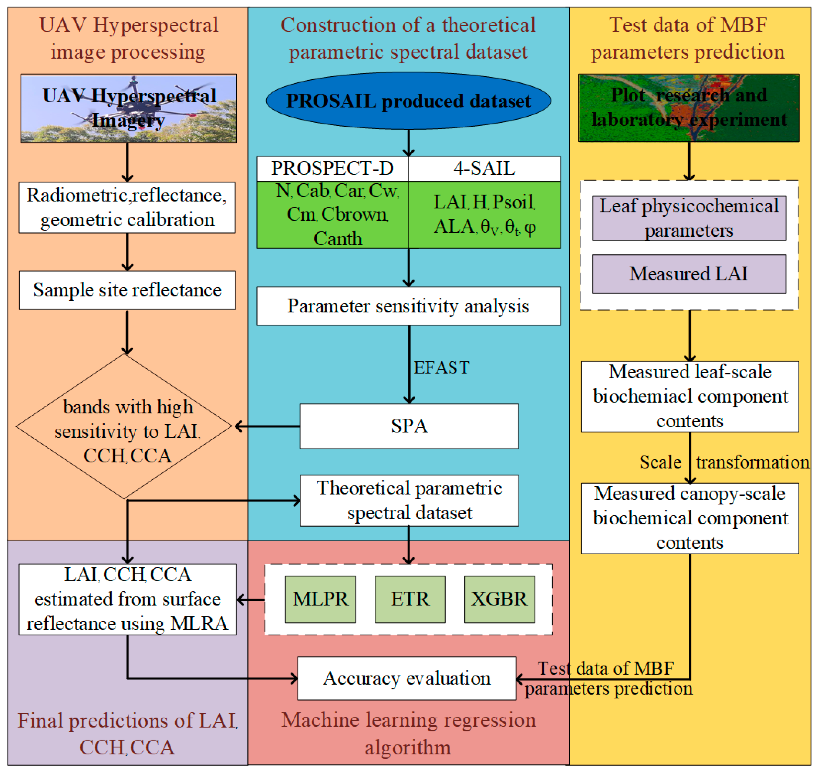
2.3. Research Methodology

2.3.1. Introduction to the PROSAIL Model

To more accurately model the spectral response of plant leaves, Feret et al. [46] proposed the PROSPECT5 model in 2008; this model could be used to distinguish the effects of different pigments on reflectance by introducing parameters such as carotenoids and chlorophyll a/b ratio [47]. Feret et al. [48] proposed the PROSPECT-D model on the basis of the PROSPECT5 model and utilized the physical principle of light–matter interaction to simulate the interaction between light and a single leaf; this further improved the model’s performance and applicability. To address the problems of ‘specular reflection’ and ‘hot spots’ of leaves in remote sensing of vegetation neglected by the SAIL model, Verhoef et al. [49] proposed the 4SAIL model, which was more applicable and optimized the model. Therefore, in this study, PROSAIL refers to the combination of two models, PROSPECT-D and 4SAIL, and the equations of the two models are shown in Equations (5) and (6).

$$\left(\rho ,\tau \right)=PROSPECT-\mathrm{D}\left(N,C_{AB},C_{AR},{{C_{ant\mathrm{h}},C}_{brown},C}_w,C_m\right)$$

(5)

$${\rho }_c=4SAIL\left(LAI,\rho ,\tau ,Hot,P_{soil},{\theta }_v,{\theta }_t,\phi \right)$$

(6)

PROSAIL characterizes the vegetation canopy using SAIL and the leaves with PROSPECT; to achieve this, a range of model input parameters are needed. In this study, a priori knowledge of field observations and sensor configurations was used to determine the range of model input parameters, as detailed in

Table 1. PROSAIL model input parameters.

Model	Parameter	Symbol	Value of Range	Unit
PROSPECT-D	Leaf structure parameter	N	1–2.5	—
	Chlorophyll content	CAB	0–60	μg·cm−2
	Carotenoid content	CAR	0–30	μg·cm−2
	Total anthocyanin content	Canth	0	μg·cm−2
	Brown pigments	Cbrown	0.1	—
	Water content	Cw	0.001–0.009	g·cm−2
	Dry matter content	Cm	0.001–0.009	g·cm−2
4-SAIL	Leaf area index	LAI	0–7	m2·m−2
	Hot-spot parameter	H	0–0.0009	—
	Soil reflectivity	Psoil	0–1	—
	Average leaf angle	ALA	45	degree
	View zenith angle	θv	0	degree
	Solar zenith angle	θt	27	degree
	Relative azimuth angle	φ	0	degree

.

2.3.2. Global Sensitivity Analysis Based on the EFAST Parameters

In this study, the extended Fourier amplitude sensitivity test (EFAST) method was used to analyze the sensitivity of each band of spectral data to the parameters of the PROSAIL model. This approach is a universal sensitivity assessment technique formed by integrating the strengths of Sobol’s method with EFAST, centered on breaking down variance [50]. Utilizing this method, the impact of individual input variables on the model is quantified by determining the primary sensitivity index (S_i) along with the overall sensitivity index (S_Ti); here, Si is the degree of influence on the output by considering only the change in a single parameter and is measured through the calculated partial derivatives of parameter changes on output changes, and S_Ti accounts for the interaction effects between the parameters.

2.3.3. Characterization Band Selection

In this study, the successive projections algorithm (SPA) was used for feature band extraction of simulated MBF spectrally sensitive band reflectance data. SPA was proposed for use in solving the covariance problem by selecting the wavelengths with the least redundancy of spectral information [51]. This algorithm selected the variable with the least redundant information by performing a simple operation in vector space [52].

The SPA algorithm consists of three main steps: first, the bands that are sensitive to LAI, CCH, and CCA are selected based on the EFAST results to form part of the spectral matrix, and a band is randomly selected from them to be added as an initial variable to the subset of variables. Second, all unselected bands are traversed and projected onto the orthogonal complementary space of the selected bands using Equation (7); specifically, if a new band is highly correlated with the selected bands, the vector obtained by its projection onto the orthogonal complementary space of the selected bands will be close to the zero vector, and this new band adds almost no new information. Third, the variable with the largest projection paradigm Equation (8) is selected and added to the subset of variables selected earlier, and then the above steps are repeated until all the desired bands have been selected.

$$P_{xj}=x_j-x_s^T{x}_s{\left(x_s^T{x}_s\right)}^{-1}{x}_j$$

(7)

$$N_j=\left|\right|P_{xj}\left|\right|$$

(8)

where $P_{xj}$ is the projection of the jth unselected variable into the orthogonal complementary space of the selected variable, $x_j$ is the jth unselected variable, $x_s$ is the selected variable T denotes the transpose of the matrix, ⁻¹ denotes the inverse matrix, and $N_j$ is the weight criterion of the jth variable selected according to the projection paradigm.

2.3.4. Introduction to Machine Learning Models

• MLPR

The learning of the MLPR model occurs through the backpropagation algorithm. In each training iteration, the model first backpropagates the input, calculates the error between the predicted value and the true target value, and then backpropagates this error, updating the weights of the neurons to reduce the prediction error [53,54]. Thus, this model is able to naturally handle complex nonlinear relationships between input features and is very suitable for handling a variety of complex regression problems.

• ETR

The ETR is an extreme random tree proposed by Geurts et al. [53] and belongs to a variant of random forest. In extreme random trees, instead of selecting the optimal features, the decision tree splits by finding the split point in a randomly selected set of features with a random threshold. This randomization process helps to reduce the variance of the decision tree and increase the diversity of the model, which, in turn, improves the overall performance of the integration. Therefore, extremely randomized trees exhibit good robustness to noise and outliers.

Parameter inversion using ETR determines parameters such as the number of trees in the extreme random tree n_estimators, the maximum depth max_depth, and the number of features that can be considered at each node max_features. In this study, the ExtraTreesRegressor model [54] was constructed based on the scikit-learn library in the Python 3.7 program, and the parameters of ETR were optimized by using the GridSearchCV function and the fivefold cross-validation method and by optimizing the abovementioned parameters using the coefficient of determination (R²) and root mean square error (RMSE) pairs.

• XGBR

The XGBR is an alternative method for predicting the dependent variable [55] and was constructed as an improvement on the gradient boosting decision tree (GBDT) algorithm, a class of integrated models. XGBoost reduces the search space mainly by learning the feature distribution of each data point to generate new branches, which improves the computational speed, and XGBoost adds regular terms to reduce the overfitting of the model at the decision tree construction stage. In the modeling process of this study, the GridSearchCV function and the fivefold cross-validation method are used to optimize each parameter of the XGBR and by optimizing the model parameters with the R² and RMSE pairs.

2.3.5. PROSAIL_MLRA Model Construction

In this study, in order to traverse each parameter combination, we generated 100,000 sets of parameter combinations based on the PROSAIL radiative transfer model and simulated the MBF reflectance corresponding to the parameter combinations on the basis of the EFAST global sensitivity analysis and SPA eigen-band extraction and constructed a theoretical MBF reflectance spectral dataset, i.e., “LAI-CCH-CCA-canopy Reflectance”. Then, with 80% of the data as the training set and 20% of the data as the validation set, the MBFLAI, CCH, and CCA inversion models were constructed using the three machine learning methods, MLPR, ETR, and XGBR, respectively. Finally, the constructed machine models were used to invert MBF LAI, CCH, and CCA from UAV hyperspectral data and validated with measured LAI, CCH, and CCA data, whose evaluation indices are shown in Equations (9)–(11).

$$R^2=1-\sum _{i=1}^n{\left(y_i-\widehat{y}\right)}^2/\sum _{i=1}^n{\left(y_i-\overline{y}\right)}^2$$

(9)

$$RMSE=\sqrt{\raisebox{1ex}{$\sum _{i=1}^n{\left(y_i-\widehat{y}\right)}^2$}\!\left/ \!\raisebox{-1ex}{$n$}\right.}$$

(10)

$$rRMSE=\frac{RMSE}{\overline{y}}\times 100\%$$

(11)

The metrics used to assess the accuracy of the model include the coefficient of R², the RMSE, and the relative root mean square error (rRMSE). $y_i$ is the actual observation, $\widehat{y}$ is the model prediction, and $\overline{y}$ is the average of the observations. In general, higher values of R² and lower values of RMSE and rRMSE indicate better performance of the model. The overall technical flowchart of this study is shown in Figure 2.

3. Results

3.1. Sensitivity of Canopy Reflectance Spectra to PROSAIL Model Input Parameters

Figure 3 shows the results of the sensitivity analysis of the LAI, CAB, and CAR parameters conducted using the EFAST global sensitivity analysis method. In the spectral range of 400–1000 nm, the degree of Si contribution of different parameters to the spectral reflectance is shown in Figure 3a. The contribution of LAI to the spectral reflectance of moso bamboo was the largest in the ranges of 400–490 nm and 710–1000 nm, with an average contribution of 78%. CAB had the largest effect on the change in reflectance in the range of 530–710 nm, with an average contribution of approximately 75%. CAR had a large effect on the change in reflectance from 490 to 530 nm, with an average contribution of approximately 88%, followed by the contribution of equivalent water thickness in the 700–1300 nm band, with an average of 20%, and the equivalent water thickness Cw and the dry matter content Cm had the smallest contribution to the spectral reflectance and the lowest sensitivity in the 600–700 nm band. Similarly, the overall degree of contribution of different parameters to the S_Ti of spectral reflectance in Figure 3b had a similar characteristic to S_i.

Through the above analysis, LAI, CAB, and CAR had a greater influence on the canopy reflectance of moso bamboo; these were set as the variable input parameters, and the remaining parameters were set as constants. The ranges of values of LAI, CAB, and CAR were determined with reference to the actual measurement data and previous studies [9], and the variable and constant input parameters of the PROSAIL model were determined as provided in

Table 2. PROSAIL model parameterization.

Symbol	Min	Max	Unit
LAI	0.1	7	m2·m−2
CAB	7	55	μg·cm−2
CAR	0.8	10	μg·cm−2
Cw	0.0035	0.0035	g·cm−2
Cm	0.005	0.005	g·cm−2
H	0.0003	0.0003	—
Psoil	0.25	0.25	—
N	1.5	1.5	—

. According to the determined model input parameters, the PROSAIL model was used to simulate the canopy reflectance of bamboo forest to obtain the simulated dataset. From Figure 4a,b, the simulated canopy reflectances of MBF on-years and off-years under the optimized parameters were relatively consistent with the observed reflectances.

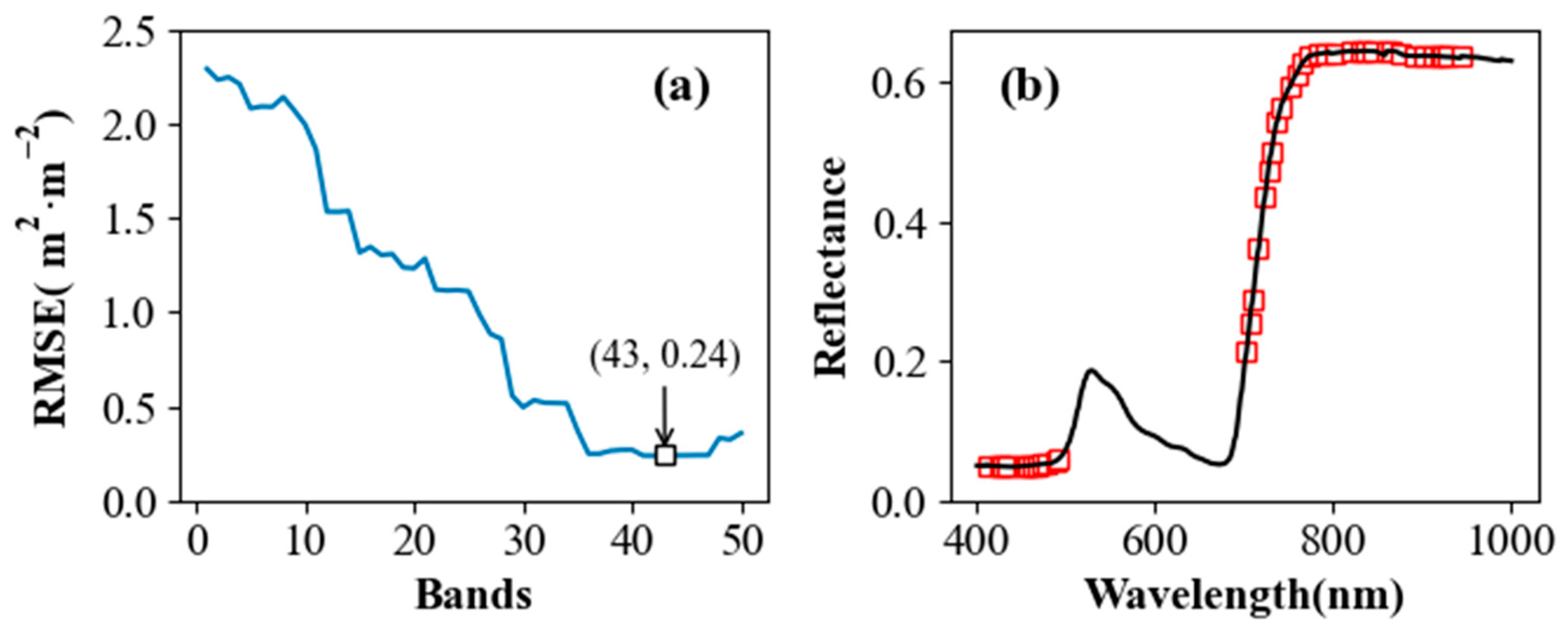
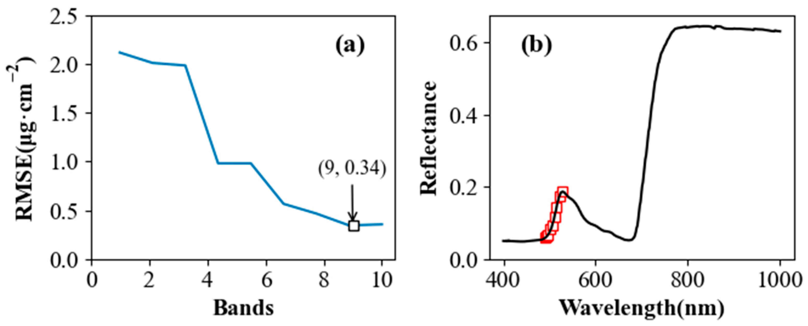
3.2. Selection of the Bands for the Characterization of the Moso Bamboo Canopy Parameters

Based on the spectral range of the UAV hyperspectral data (400~1000 nm) and the parameter sensitivity analysis, the wavelength range of 400~490 and 710~1000 nm was selected as the spectral data intervals for MBF canopy LAI inversion. The wavelength ranges of 530~710 nm were selected as the spectral data intervals for the CCH inversion of MBF. The wavelength range of 490~530 nm was selected as the spectral data intervals for the CCA inversion of MBF.

In this study, the simulated spectra were analyzed using the SPA algorithm to extract the characteristic bands of the canopy parameters, and the spectral features were screened using the RMSE values. Figure 5, Figure 6 and Figure 7 show the spectral feature bands of the MBF canopy parameters LAI, CCH, and CCA screened using the SPA algorithm. As the number of optimal bands increased, the overall RMSE tended to decrease; therefore, in this study, the number of feature bands for LAI, CCH, and CCA of moso bamboo were determined to be 43, 21, and 9, respectively, when the RMSE values reached the minimum of 0.24 m²/m², 0.41 μg/cm², and 0.34 μg/cm², respectively, as shown in Figure 5a, Figure 6a and Figure 7a, and the selected feature bands are shown in Figure 5b, Figure 6b and Figure 7b.

3.3. Comparison of the Inversion Models for the Canopy Parameters of the MBF

3.3.1. Inversion of the Canopy Parameters Based on MLPR

Table 3. Parameter settings used for MLPR model.

Variable Name	Values/Range	Best Combination
		LAI	CCH	CCA
Hidden layer sizes	[(50,), (50, 50), (100, 50), (100, 100), (50, 50, 50), (50, 100, 50)]	(50, 50)	(50, 100, 50)	(100, 100)
Activation	[Identity, logistic, tanh, relu]	relu	tanh	relu
Alpha	[0.0001, 0.001, 0.01, 0.05]	0.001	0.05	0.001
Learning rate initial	[0.0001, 0.001, 0.01, 0.05]	0.01	0.001	0.01

shows the hyperparameter optimization results of the MLPR model using the grid search algorithm (GridSearchCV). Figure 8a–c show the results of MLPR-based hyperparameter optimization for modeling the MBF canopy parameters LAI, CCH, and CCA. As shown in these figures, the model training accuracies R² of PROSAIL-MLPR are 0.9969, 0.9970, and 0.9937, with rRMSE of 2.75%, 4.82%, and 6.35%, respectively; the model validation accuracies R² are 0.9962, 0.9965, and 0.9934, with rRMSE of 2.65%, 4.16%, and 6.54%.

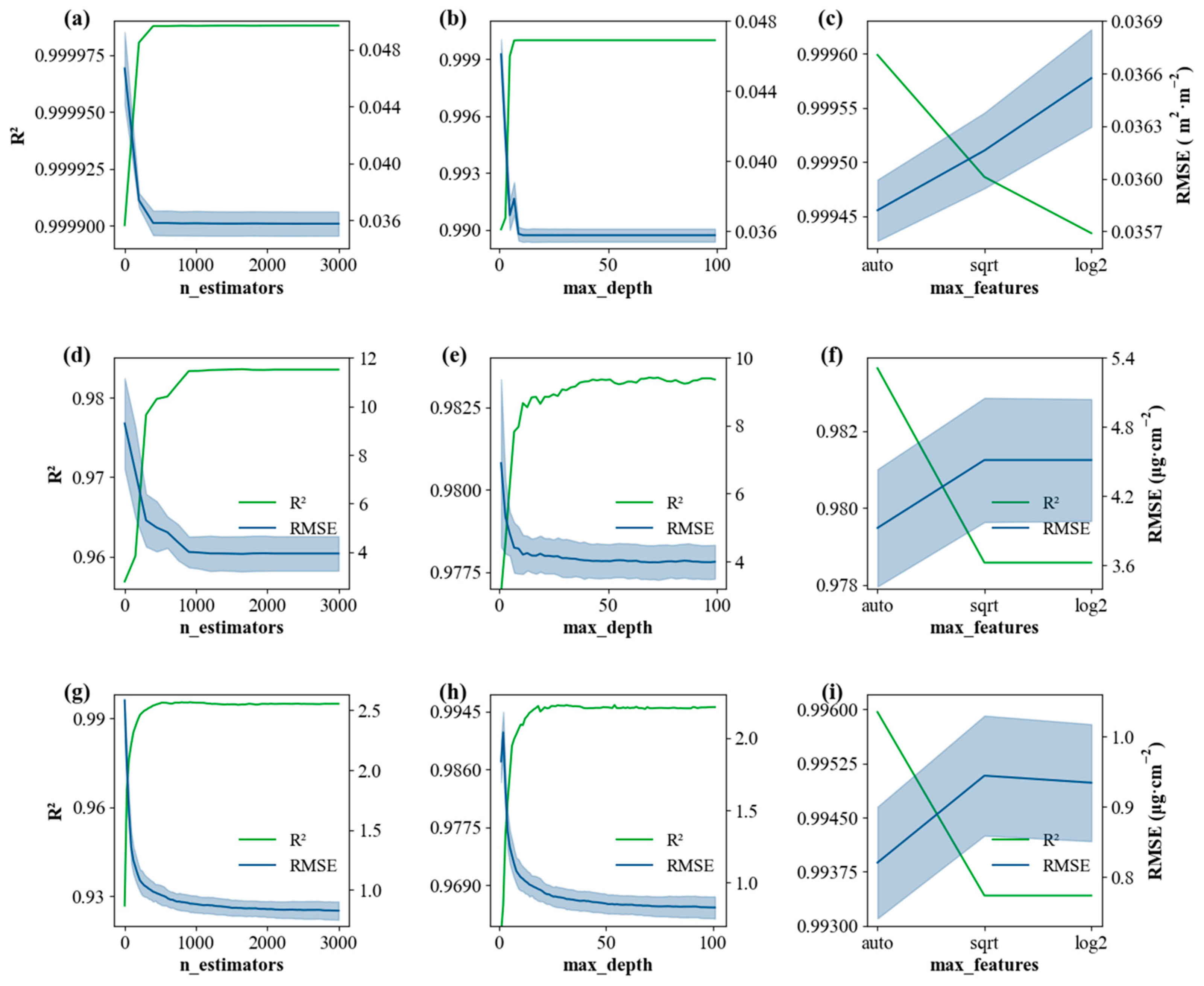
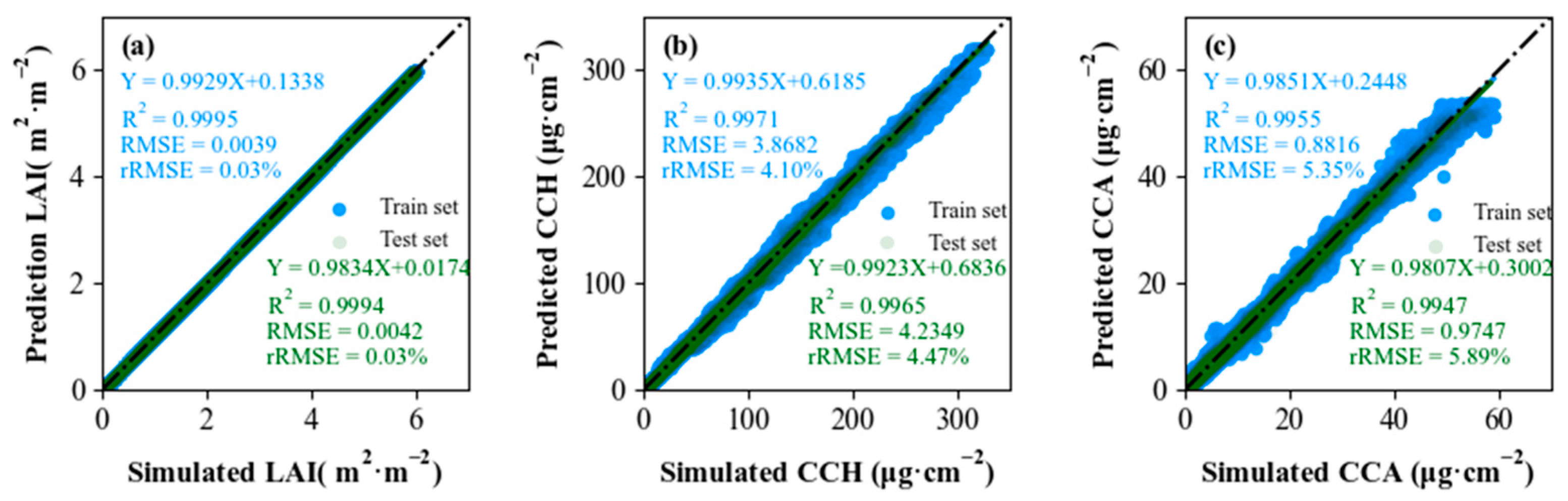
3.3.2. ETR-Based Inversion of the Canopy Parameters

Figure 9 shows the variation curves of canopy parameters R² and RMSE with the values of n_estimators, max_depth, and max_features. When the value of n_estimators was greater than 500, the R² and RMSE values of the canopy parameter LAI generally stabilized, as shown in Figure 9a. Then, max_depth was optimized after determining n_estimators. Figure 9b shows the stability of R² and RMSE for max_depth greater than 20. Finally, as shown in Figure 9c, RMSE reached a minimum value of 0.0053 m²/m², and R² reached a maximum value of 0.9998 when max_features was set to ‘auto.’ Similarly, the optimal hyperparameters for the canopy parameter CCH were obtained as follows: n_estimators = 2000, max_depth = 50, max_features = 20, max_depth = 20, and max_features = ‘auto’, and the RMSE gradually decreased to a minimum value of 4.26 μg/cm² with a maximum R² value of 0.9998. Similarly, the optimal hyperparameters for the canopy parameter CCA are obtained: n_estimators = 2000, max_depth = 80, and max_features = ‘auto’, and the RMSE gradually decreased to a minimum value of 0.94 μg/cm², with a maximum R² value of 0.9998.

Figure 10a–c show the results of ETR based on hyperparameter optimization for modeling the MBF canopy parameters LAI, CCH, and CCA. As shown in these figures, the model training accuracies R² of PROSAIL-ETR were 0.9995, 0.9872, and 0.9955, with rRMSE values of 0.03%, 4.1%, and 5.35%, respectively; the model validation accuracies R² were 0.994, 0.9965, and 0.9947, with rRMSE values of 0.03%, 4.47%, and 5.89%, respectively.

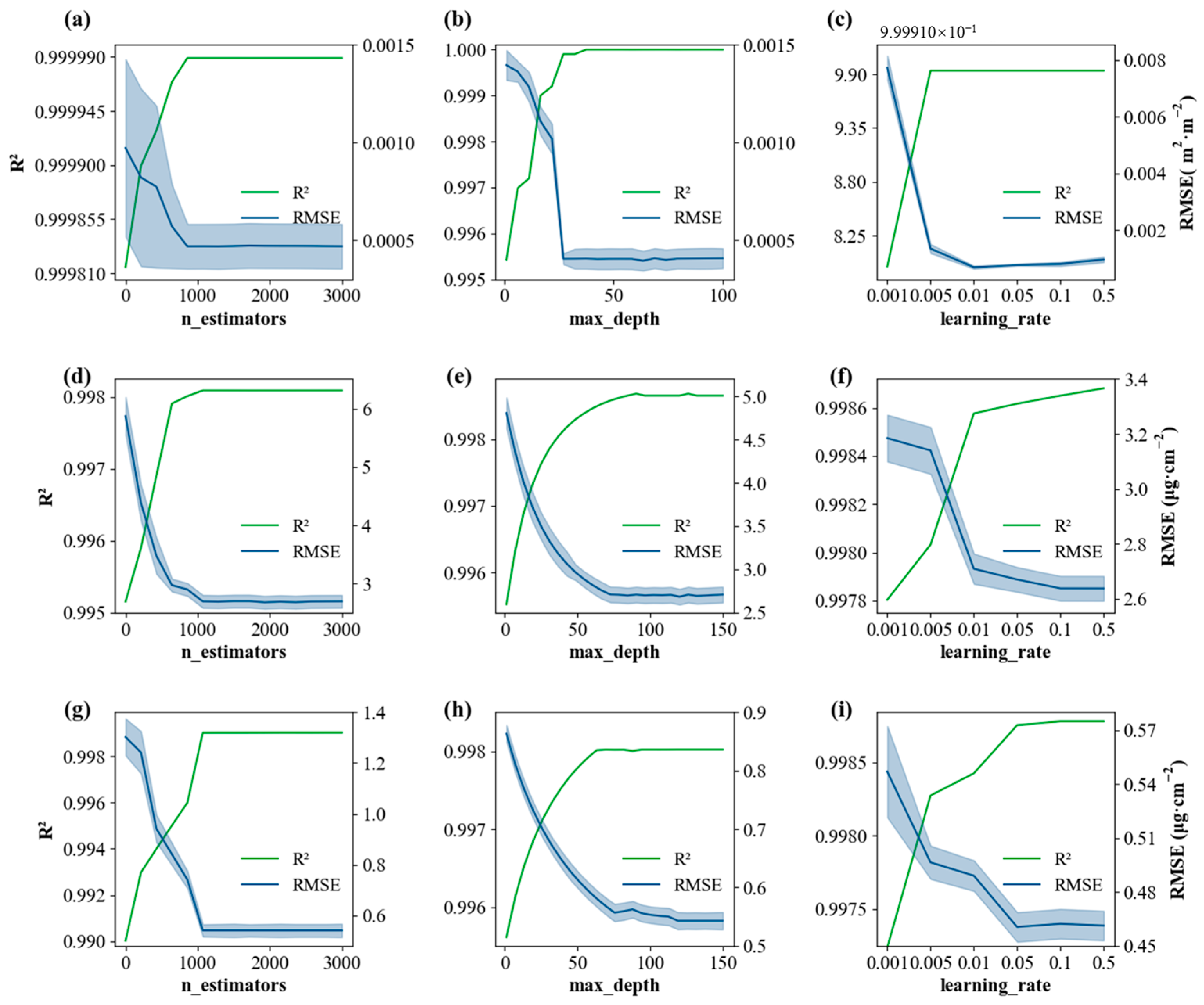
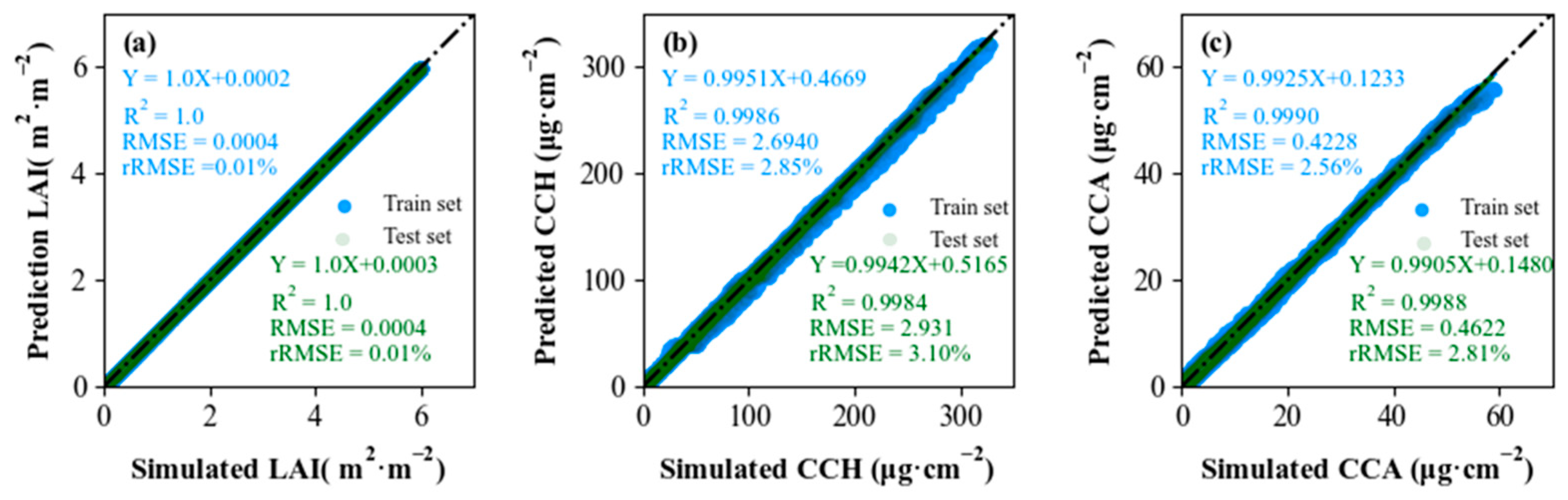
3.3.3. XGBR-Based Inversion of the Canopy Parameters

Figure 11 shows the variation curves of canopy parameters R² and RMSE with the values of n_estimators, max_depth, and learning_rate. When the value of n_estimators was greater than 1000, the R² and RMSE values of the canopy parameter LAI generally stabilized, as shown in Figure 11a. Then, max_depth was optimized after determining n_estimators. Figure 11b shows the stability of R² and RMSE for max_depth greater than 30. Finally, as shown in Figure 11c, the RMSE reached a minimum value of 0.0001 m²/m² and a maximum value of R² of 1.0 when the learning_rate was greater than 0.05. Similarly, the optimal hyperparameters for the canopy parameter CCH were obtained as follows: n_estimators = 2000, max_depth = 80, and learning_rate = 0.5. The RMSE gradually decreased to a minimum value of 2.638 μg/cm² and a maximum value of R² of 0.9987. The optimal hyperparameters for the canopy parameter CCA were as follows: n_estimators = 1200, max_depth = 140, learning_rate = 0.1, gradual RMSE decrease to a minimum value of 0.4613 μg/cm², and a maximum value of R² of 0.9988.

Figure 12a–c show the results of modeling the MBF canopy parameters LAI, CCH, and CCA by XGBR based on hyperparameter optimization. As shown in these figures, the model training accuracies R² of PROSAIL_XGBR were 1.0, 0.9986, and 0.9990, with rRMSE values of 0.01%, 2.85%, and 2.56%, respectively; the model validation accuracies R² were 1.0, 0.9984, and 0.9988, with rRMSE values of 0.01%, 3.10%, and 2.81%, respectively.

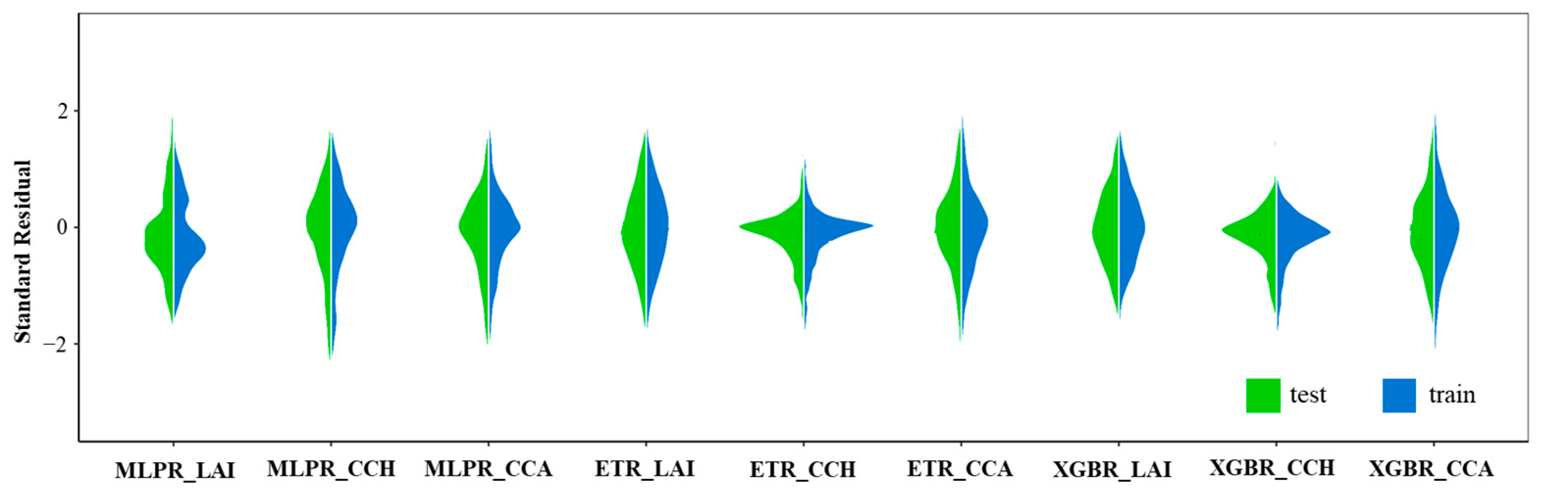
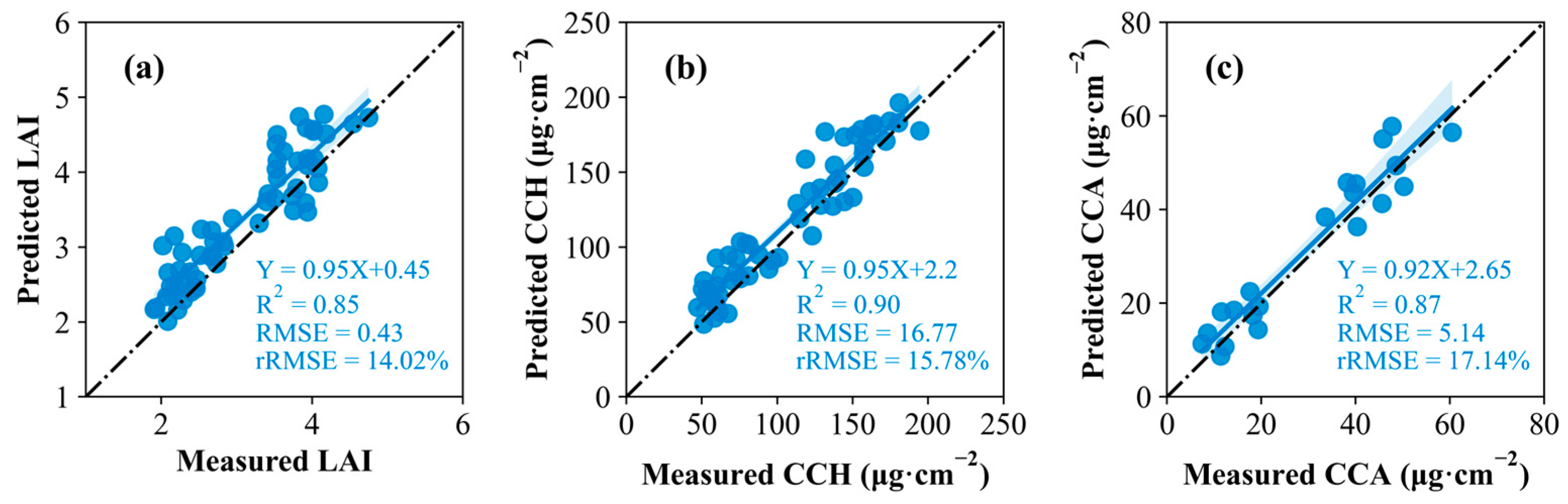
3.3.4. Comparison of Model Result

Figure 13 shows the distribution of standardized residuals of training and validation accuracies of the three MLRAs for estimating the three bamboo forest canopy parameters, and the standardized residuals of the sample canopy parameters of the three models were in the range of 2.5 to 2, which was normally distributed. These results indicated that all three models had better stabilities and generalization abilities in estimating the bamboo forest canopy parameters.

Table 4. Evaluation of canopy parameters for different models.

	Model	LAI			CCH			CCA
		R2	RMSE (m2/m2)	rRMSE (%)	R2	RMSE (μg/cm2)	rRMSE (%)	R2	RMSE (μg/cm2)	rRMSE (%)
Train	MLPR	0.9969	0.0658	2.15	0.9970	4.6566	4.82	0.9937	1.0471	6.35
	ETR	0.9995	0.0039	0.03	0.9971	3.8682	4.1	0.9955	0.8816	5.13
	XGBR	1.0	0.0004	0.01	0.9986	2.6940	2.85	0.9990	0.4228	2.56
Test	MLPR	0.9962	0.0670	2.65	0.9965	6.6579	4.16	0.9934	1.1251	6.54
	ETR	0.9994	0.0042	0.03	0.9965	4.2349	4.47	0.9947	0.9747	5.89
	XGBR	1.0	0.0004	0.01	0.9984	2.9310	3.1	0.9988	0.4622	2.81

shows the differences in the inversion performance of the three models for the bamboo forest canopy parameters LAI, CCH, and CCA, and all three models could attain the estimation of bamboo forest canopy parameters with higher accuracy. Based on these results, the performance of PROSAIL_XGBR was better than those of both the PROSAIL_MLPR and PROSAIL_ETR models.

As shown in Table 4, the best machine learning model for estimating bamboo forest canopy parameters based on UAV hyperspectral remote sensing data was PROSAIL_XGBR. The accuracies of LAI, CCH, and CCA in the PROSAIL_MLPR model inversion of LAI, CCH, and CCA were evaluated by using measured LAI, CCH, and CCA of the 59 sample plots, as shown in Figure 14a–c. The results showed that PROSAIL_MLPR inversions of LAI, CCH, and CCA had a good correlation with the measured LAI, CCH, and CCA with model validation accuracies of R² of 0.85, 0.90, and 0.87 and rRMSEs of 14.02%, 15.78%, and 17.14%, respectively.

Figure 15a–c show the spatial distribution of canopy parameter inversion for the area, with non-vegetated areas in blue and vegetated areas in color. The on-year LAI values of MBF ranged from 3.15 to 4.53 m²/m², averaging 3.84 m²·m⁻², while the LAI values ranged from 1.87 to 2.94 m²/m² in off-years, with an average of 2.37 m²·m⁻². Furthermore, the CCH values of MBF in on-years and off-years ranged from 106.44 to 194.31 µg/cm² and 43.46 to 100.86 µg/cm², respectively, with average values of 71.91 µg/cm² and 150.12 µg/cm², respectively. The CCA ranged from 33.54 to 60.53 µg/cm² in the on-years and from 6.70 to 20.32 µg/cm² in the off-years, averaging 45.38 µg/cm² in the on-years and 13.40 µg/cm² in the off-years. The inverted MBF on-years and off-years canopy parameters were consistent with the moso bamboo growth conditions at the sample site.

4. Discussion

4.1. Impact of Parametric Sensitivity Analysis on PROSAIL Modeling

Parameter sensitivity analysis has been recognized as a tool used to identify key parameters of a model and can help to understand the model structure and develop effective inversion strategies [56]. In this study, the global sensitivity analysis EFAST was utilized to analyze the PROSAIL model parameters, and the results are shown in Figure 3. LAI significantly contributed throughout the band process [57], especially in the near-infrared band, where the average contribution of S_i and S_Ti reached 78% and 57%, respectively. In contrast, the contributions of CAB and CAR were mainly concentrated in the blue and red light phases due to their specific spectral absorption properties, and the average contributions of S_i and S_Ti reached 75% and 56%, respectively. CAR was mainly concentrated in the blue and green light bands, and the average contributions of S_i and S_Ti were 88% and 63%. The relevant bands are also the main regions where CAB and CAR absorb light, respectively [58]. LAI was the most important structural driver and played a key role in the structure and physiology of vegetation, and CAB and CAR were important pigments for the photosynthesis of vegetation; thus, we could understand the information on the optical properties, the physiological processes and the structural changes of vegetation by studying the changes in LAI, CAB, and CAR. The changes in LAI, CAB, and CAR were studied to understand the information on the optical properties, physiological processes, and structural changes of vegetation. In the EFAST process, all metrics were more or less affected by confounding variables and not fully sensitive to a single target variable because the canopy reflectance was the result of complex interactions between the absorbance and scattering of biochemicals and structural variables [59,60]; additionally, the different biochemical components within the leaf correlations, as well as the saturation of parameters by preferred traits, affected the sensitivity between biochemical parameters.

4.2. Influence of Spatial Resolution of UAV Images on Canopy Parameter Inversion

The PROSAIL model was initially based on the turbid medium assumption to study the canopy and was suitable for a homogeneous vegetation canopy, i.e., most pixels are ‘pure’ [61,62]. High-resolution images can satisfy the need to obtain more pure pixels [63,64], and in this study, we used hyperspectral images with a spatial resolution of 0.1 m and could obtain more ‘pure’ pixels to satisfy the inversion of the PROSAIL_MLRA model. The PROSAIL_MLRA model was different from other empirical methods that needed several ground measurement datasets for modeling and used simulated datasets; however, this model was prone to data redundancy and spectral covariance in the simulation-generated sample data, affecting the model efficiency [65]. To obtain accurate MBF canopy parameter estimates, the optimal spectral bands needed to be screened. A higher spectral resolution correlated to a better band selection, lower uncertainty of the model parameters, and better accuracy and stability of the parameter inversion [66]. SPA determined the optimal band by the RMSE minimum, which reduced covariance interference and greatly simplified the modeling process. The wavelengths that best reflected the parameters LAI, CAB, and CAR were obtained to reduce the complexity of the data and the interference of irrelevant information, thus improving the accuracy and stability of the inversion model of MBF canopy parameters.

4.3. Mixed Inversion Modeling of Canopy Parameters

Table 4 and Figure 14 show that PROSAIL_MLRA significantly improves the accuracy of parameter inversion with an R² value as high as 0.99, which is consistent with the results of Wang et al., 2021 [67]. By comparing and analyzing the three MBF canopy parameter estimation methods for the PROSAIL_MLRA model, PROSAIL_XGBR outperformed PROSAIL_ETR, which, in turn, was superior to PROSAIL_MLPR (Table 4). The tree-based integration algorithms (e.g., ETR, XGBR) performed better than the MLPR in terms of performance [68,69]. The better performance of tree-based integration algorithms stemmed from their flexibility and strength in handling all data types. They could handle nonlinearities in the dataset and complex relationships between dependent and independent variables; the outliers were effectively modeled where other models might fail to model them. The integrated models could capture minute details of a dataset that were also within a training dataset of limited size. They also greatly reduced variance, and their ability to effectively handle missing values further improved their robustness. Among the integrated tree-based algorithms, the XGBR algorithm provided the best R² and the lowest RMSE values (Figure 12). ETR is a bagging model, and XGBR is a boosting model, where the boost-based ensemble severely penalizes the wrong prediction points and improves the bias. Therefore, the performance was slightly better than that of the integrated bagging-based model.

5. Conclusions

In this study, a novel hybrid model for estimating MBF canopy parameters was innovatively constructed by combining the PROSAIL radiative transfer model with an MLRA. This approach achieved the high-precision inversion of the MBF canopy parameters, including LAI, CCH, and CCA. Our findings revealed the spectral sensitivity nuances across different wavelengths, identifying specific bands (400–490 and 710–1000 nm for LAI, 530–710 nm for chlorophyll, and 490–530 nm for carotenoids) as pivotal for parameter estimation. By employing the successive projections algorithm (SPA), we effectively narrowed down the required bands, demonstrating improved inversion performance with RMSE values of 0.24 m²/m² for LAI, 0.41 µg/cm² for CCH, and 0.34 µg/cm² for CCA. The introduction of machine learning algorithms, particularly the PROSAIL_XGBR model, achieves high prediction accuracies with R² values exceeding 0.85 for all parameters under investigation. This underscores the potential of our hybrid approach in delivering spatially explicit, high-resolution assessments of forest health and productivity.

Despite these achievements, this study still has some limitations. The current model fails to adequately distinguish between direct vegetation signals and indirect effects caused by environmental factors such as shade, varying light conditions, and atmospheric disturbances, which may introduce uncertainty in field applications. Future studies should address these limitations by incorporating more environmental variables and validating the model in a wider range of geographic and ecological settings to enhance its utility in forest monitoring and management.

References

1. Croft, H.; Chen, J.M.; Wang, R.; Mo, G.; Luo, S.; Luo, X.; He, L.; Gonsamo, A.; Arabian, J.; Zhang, Y.; et al. The global distribution of leaf chlorophyll content. Remote Sens. Environ. 2020, 236, 111–479. [Google Scholar] [CrossRef]
2. Skidmore, A.K.; Coops, N.C.; Neinavaz, E.; Ali, A.; Schaepman, M.E.; Paganini, M.; Kissling, W.D.; Vihervaara, P.; Darvishzadeh, R.; Feilhauer, H.; et al. Priority list of biodiversity metrics to observe from space. Nat. Ecol. Evol. 2021, 5, 896–906. [Google Scholar] [CrossRef] [PubMed]
3. Du, H.; Zhou, G.; Mao, F.; Han, L. Quantitative Inversion of Bamboo Forest Parameters by Multi-Source Remote Sensing; Science Press: Beijing, China, 2022; p. 142. [Google Scholar]
4. Sun, J.; Wang, L.; Shi, S.; Li, Z.; Yang, J.; Gong, W.; Wang, S.; Tagesson, T. Leaf pigment retrieval using the PROSAIL model: Influence of uncertainty in prior canopy-structure information. Crop J. 2022, 10, 1251–1263. [Google Scholar] [CrossRef]
5. Fang, H.; Baret, F.; Plummer, S.; Schaepman, G. An Overview of Global Leaf Area Index (LAI): Methods, Products, Validation, and Applications. Rev. Geophys. 2020, 57, 739–799. [Google Scholar] [CrossRef]
6. Wu, G.; Jiang, C.; Kimm, H.; Wang, S.; Bernacchi, C.; Moore, C.E.; Suyker, A.; Yang, X.; Magney, T.; Frankenberg, C.; et al. Difference in seasonal peak timing of soybean far-red SIF and GPP explained by canopy structure and chlorophyll content. Remote Sens. Environ. 2022, 279, 113104. [Google Scholar] [CrossRef]
7. Zhang, L.; Gao, H.; Zhang, X. Combining Radiative Transfer Model and Regression Algorithms for Estimating Aboveground Biomass of Grassland in West Ujimqin, China. Remote Sens. 2023, 15, 2918. [Google Scholar] [CrossRef]
8. Gara, T.W.; Darvishzadeh, R.; Skidmore, A.K.; Wang, T.; Heurich, M. Accurate modelling of canopy traits from seasonal Sentinel-2 imagery based on the vertical distribution of leaf traits. ISPRS J. Photogramm. Remote Sens. 2019, 157, 108–123. [Google Scholar] [CrossRef]
9. Ji, J.; Li, X.; Du, H.; Mao, F.; Fan, W.; Xu, Y.; Huang, Z.; Wang, J.; Kang, F. Multiscale leaf area index assimilation for Moso bamboo forest based on Sentinel-2 and MODIS data. Int. J. Appl. Earth Obs. Geoinf. 2021, 104, 102519. [Google Scholar] [CrossRef]
10. Zhu, J.; Yin, Y.; Lu, J.; Warner, T.A.; Xu, X.; Lyu, M.; Wang, X.; Guo, C.; Cheng, T.; Zhu, Y.; et al. The relationship between wheat yield and sun-induced chlorophyll fluorescence from continuous measurements over the growing season. Remote Sens. Environ. 2023, 298, 113791. [Google Scholar] [CrossRef]
11. Liang, S. Quantitative Remote Sensing of Land Surfaces; John Wiley & Sons: Hoboken, NJ, USA, 2003; pp. 1–534. [Google Scholar] [CrossRef]
12. Kang, F.; Li, X.; Du, H.; Mao, F.; Zhou, G.; Xu, Y.; Huang, Z.; Ji, J.; Wang, J. Spatiotemporal Evolution of the Carbon Fluxes from Bamboo Forests and their Response to Climate Change Based on a BEPS Model in China. Remote Sens. 2022, 14, 366. [Google Scholar] [CrossRef]
13. Yu, K.; Lenz-Wiedemann, V.; Chen, X.P.; Bareth, G. Estimating leaf chlorophyll of barley at different growth stages using spectral indices to reduce soil background and canopy structure effects. Isprs J. Photogramm. Remote Sens. 2014, 97, 58–77. [Google Scholar] [CrossRef]
14. Asner, G.P.; Mascaro, J.; Anderson, C.; Knapp, D.E.; Martin, R.E.; Kennedy-Bowdoin, T.; van Breugel, M.; Davies, S.; Hall, J.S.; Muller-Landau, H.C.; et al. High-fidelity national carbon mapping for resource management and REDD+. Carbon Balance Manag. 2015, 8, 7. [Google Scholar] [CrossRef] [PubMed]
15. Zhang, Y.; Migliavacca, M.; Penuelas, J.; Ju, W. Advances in hyperspectral remote sensing of vegetation traits and functions. Remote Sens. Environ. 2021, 252, 112121. [Google Scholar] [CrossRef]
16. Guo, K.; Li, X.; Du, H.; Mao, F.; Ni, C.; Chen, Q.; Xu, Y.; Huang, Z. Wavelet Vegetation Index to Improve the Inversion Accuracy of Leaf V25cmax of Bamboo Forests. Remote Sens. 2023, 15, 2362. [Google Scholar] [CrossRef]
17. Chen, Z.; Jia, K.; Xiao, C.; Wei, D.; Zhao, X.; Lan, J.; Wei, X.; Yao, Y.; Wang, B.; Sun, Y.; et al. Leaf Area Index Estimation Algorithm for GF-5 Hyperspectral Data Based on Different Feature Selection and Machine Learning Methods. Remote Sens. 2020, 12, 2110. [Google Scholar] [CrossRef]
18. Li, Y.; Liang, S. Evaluation of Reflectance and Canopy Scattering Coefficient Based Vegetation Indices to Reduce the Impacts of Canopy Structure and Soil in Estimating Leaf and Canopy Chlorophyll Contents. IEEE Trans. Geosci. Remote Sens. 2023, 61, 4403015. [Google Scholar] [CrossRef]
19. Houborg, R.; Fisher, J.B.; Skidmore, A.K. Advances in remote sensing of vegetation function and traits. Int. J. Appl. Earth Obs. Geoinf. 2015, 43, 1–6. [Google Scholar] [CrossRef]
20. He, L.; Ren, X.; Wang, Y.; Liu, B.; Zhang, H.; Liu, W.; Feng, W.; Guo, T. Comparing methods for estimating leaf area index by multi-angular remote sensing in winter wheat. Sci. Rep. 2020, 10, 13943. [Google Scholar] [CrossRef] [PubMed]
21. Li, H.; Fan, W.; Yu, Y.; Yang, Y. Leaf area index retrieval based on prospect, liberty and geosail models. Sci. Silvae Sin. 2011, 47, 75–81. [Google Scholar] [CrossRef]
22. Duan, S.-B.; Li, Z.-L.; Wu, H.; Tang, B.-H.; Ma, L.; Zhao, E.; Li, C. Inversion of the PROSAIL model to estimate leaf area index of maize, potato, and sunflower fields from unmanned aerial vehicle hyperspectral data. Int. J. Appl. Earth Obs. Geoinf. 2014, 26, 12–20. [Google Scholar] [CrossRef]
23. Gupta, S.K.; Pandey, A.C. PROSAIL and empirical model to evaluate spatio-temporal heterogeneity of canopy chlorophyll content in subtropical forest. Model. Earth Syst. Environ. 2022, 8, 2151–2165. [Google Scholar] [CrossRef]
24. Xiao, Y.; Zhao, W.; Zhou, D.; Gong, H. Sensitivity of canopy reflectance to biochemical and biophysical variables. J. Remote Sens. 2015, 19, 368–374. [Google Scholar] [CrossRef]
25. Ma, J.; Huang, S.; Li, J.; Xi, L. Global sensitivity analysis of parameters in the PROSAIL model based on modified sobol’s method. Bull. Surv. Mapp. 2016, 3, 33–35. [Google Scholar] [CrossRef]
26. Binh, N.A.; Hauser, L.T.; Viet Hoa, P.; Thi Phuong Thao, G.; An, N.N.; Nhut, H.S.; Phuong, T.A.; Verrelst, J. Quantifying mangrove leaf area index from Sentinel-2 imagery using hybrid models and active learning. Int. J. Remote Sens. 2022, 43, 5636–5657. [Google Scholar] [CrossRef] [PubMed]
27. Shorten, P.R.; Leath, S.R.; Schmidt, J.; Ghamkhar, K. Predicting the quality of ryegrass using hyperspectral imaging. Plant Methods 2019, 15, 63. [Google Scholar] [CrossRef] [PubMed]
28. Canova, L.d.S.; Vallese, F.D.; Pistonesi, M.F.; de Araújo Gomes, A. An improved successive projections algorithm version to variable selection in multiple linear regression. Anal. Chim. Acta 2023, 1274, 341560. [Google Scholar] [CrossRef] [PubMed]
29. Lu, D.; Chen, Q.; Wang, G.; Liu, L.; Li, G.; Moran, E. A survey of remote sensing-based aboveground biomass estimation methods in forest ecosystems. Int. J. Digit. Earth 2014, 9, 63–105. [Google Scholar] [CrossRef]
30. Meng, S.; Pang, Y.; Zhang, Z.; Jia, W. Mapping Aboveground Biomass using Texture Indices from Aerial Photos in a Temperate Forest of Northeastern China. Remote Sens. 2016, 8, 230. [Google Scholar] [CrossRef]
31. Chen, L.; Ren, C.; Zhang, B.; Wang, Z. Estimation of forest above-ground biomass by geographically weighted regression and machine learning with sentinel imagery. Forest 2018, 9, 582. [Google Scholar] [CrossRef]
32. De Sá, N.C.; Baratchi, M.; Hauser, L.T.; van Bodegom, P. Exploring the Impact of Noise on Hybrid Inversion of PROSAIL RTM on Sentinel-2 Data. Remote Sens. 2021, 13, 648. [Google Scholar] [CrossRef]
33. Jiao, Q.; Sun, Q.; Zhang, B.; Huang, W.; Ye, H.; Zhang, Z.; Zhang, X.; Qian, B. A Random Forest Algorithm for Retrieving Canopy Chlorophyll Content of Wheat and Soybean Trained with PROSAIL Simulations Using Adjusted Average Leaf Angle. Remote Sens. 2022, 14, 98. [Google Scholar] [CrossRef]
34. Liang, L.; Di, L.; Zhang, L.; Deng, M.; Qin, Z.; Zhao, S.; Lin, H. Estimation of crop LAI using hyperspectral vegetation indices and a hybrid inversion method. Remote Sens. Environ. 2015, 165, 123–134. [Google Scholar] [CrossRef]
35. Verrelst, J.; Camps-Valls, G.; Muñoz-Marí, J.; Rivera, J.P.; Veroustraete, F.; Clevers, J.G.P.W.; Moreno, J. Optical remote sensing and the retrieval of terrestrial vegetation bio-geophysical properties—A review. ISPRS J. Photogramm. Remote Sens. 2015, 108, 273–290. [Google Scholar] [CrossRef]
36. Dong, T.; Liu, J.; Qian, B.; Zhao, T. Estimating winter wheat biomass by assimilating leaf area index derived from fusion of Landsat-8 and MODIS data. Int. J. Appl. Earth Obs. Geoinf. 2016, 49, 63–74. [Google Scholar] [CrossRef]
37. Pham, L.T.H.; Brabyn, L. Monitoring mangrove biomass change in Vietnam using SPOT images and an object-based approach combined with machine learning algorithms. ISPRS J. Photogramm. Remote Sens. 2017, 128, 86–97. [Google Scholar] [CrossRef]
38. Singh, C.; Karan, S.K.; Sardar, P.; Samadder, S.R. Remote sensing-based biomass estimation of dry deciduous tropical forest using machine learning and ensemble analysis. J. Environ. Manag. 2022, 308, 114639. [Google Scholar] [CrossRef]
39. Mahato, K.D.; Kumar Das, S.S.G.; Azad, C.; Kumar, U. Machine learning based hybrid ensemble models for prediction of organic dyes photophysical properties: Absorption wavelengths, emission wavelengths, and quantum yields. APL Mach. Learn. 2024, 2, 016101. [Google Scholar] [CrossRef]
40. Zhao, D.; Zhen, J.; Zhang, Y.; Miao, J.; Shen, Z.; Jiang, X.; Wang, J.; Jiang, J.; Tang, Y.; Wu, G.; et al. Mapping mangrove leaf area index (LAI) by combining remote sensing images with PROSAIL-D and XGBoost methods. Remote Sens. Ecol. Conserv. 2022, 9, 370–389. [Google Scholar] [CrossRef]
41. Du, H.; Fan, W.; Zhou, G.; Xu, X.; Ge, H.; Shi, Y.; Zhou, Y.; Cui, R.; Lu, Y. Retrieval of Canopy Closure and LAI of Moso Bamboo Forest Using Spectral Mixture Analysis Based on Real Scenario Simulation. IEEE Trans. Geosci Remote 2011, 49, 4328–4340. [Google Scholar] [CrossRef]
42. Mao, F.; Li, P.; Zhou, G.; Du, H.; Xu, X.; Shi, Y.; Mo, L.; Zhou, Y.; Tu, G. Development of the BIOME-BGC model for the simulation of managed Moso bamboo forest ecosystems. J Environ. Manag. 2016, 172, 29–39. [Google Scholar] [CrossRef]
43. Li, X.; Du, H.; Zhou, G.; Mao, F.; Zhang, M.; Han, N.; Fan, W.; Liu, H.; Huang, Z.; He, S.; et al. Phenology estimation of subtropical bamboo forests based on assimilated MODIS LAI time series data. ISPRS J. Photogramm. Remote Sens. 2021, 173, 262–277. [Google Scholar] [CrossRef]
44. Xu, Y.; Li, X.; Du, H.; Mao, F.; Zhou, G.; Huang, Z.; Fan, W.; Chen, Q.; Ni, C.; Guo, K. Improving extraction phenology accuracy using SIF coupled with the vegetation index and mapping the spatiotemporal pattern of bamboo forest phenology. Remote Sens. Environ. 2023, 297, 113785. [Google Scholar] [CrossRef]
45. Ali, A.M.; Darvishzadeh, R.; Skidmore, A.K.; Duren, I.v.; Heiden, U.; Heurich, M. Estimating leaf functional traits by inversion of PROSPECT: Assessing leaf dry matter content and specific leaf area in mixed mountainous forest. Int. J. Appl. Earth Obs. Geoinf. 2016, 45, 66–76. [Google Scholar] [CrossRef]
46. Feret, J.-B.; François, C.; Asner, G.P.; Gitelson, A.A.; Martin, R.E.; Bidel, L.P.R.; Ustin, S.L.; le Maire, G.; Jacquemoud, S. PROSPECT-4 and 5: Advances in the leaf optical properties model separating photosynthetic pigments. Remote Sens. Environ. 2008, 112, 3030–3043. [Google Scholar] [CrossRef]
47. Zhang, L.; Li, X.; Du, H. Time series simulation of canopy reflectance in typical subtropical forests with PROSPECT5 coupled with 4SAIL model. J. Appl. Ecol. 2017, 28, 9. [Google Scholar] [CrossRef]
48. Féret, J.B.; Gitelson, A.A.; Noble, S.D.; Jacquemoud, S. PROSPECT-D: Towards modeling leaf optical properties through a complete lifecycle. Remote Sens. Environ. 2017, 193, 204–215. [Google Scholar] [CrossRef]
49. Verhoef, W.; Bach, H. Coupled soil–leaf-canopy and atmosphere radiative transfer modeling to simulate hyperspectral multi-angular surface reflectance and TOA radiance data. Remote Sens. Environ. 2007, 109, 166–182. [Google Scholar] [CrossRef]
50. Gu, C.; Du, H.; Mao, F.; Han, N.; Zhou, G.; Xu, X.; Sun, S.; Gao, G. Global sensitivity analysis of PROSAIL model parameters when simulating Moso bamboo forest canopy reflectance. Int. J. Remote Sens. 2016, 37, 5270–5286. [Google Scholar] [CrossRef]
51. Araújo, M.C.U.; Saldanha, T.C.B.; Galvão, R.K.H.; Yoneyama, T.; Chame, H.C.; Visani, V. The successive projections algorithm for variable selection in spectroscopic multicomponent analysis. Chemom. Intell. Lab. Syst. 2001, 57, 65–73. [Google Scholar] [CrossRef]
52. Han, L.; Jiang, X.; Zhou, S.; Tian, J.; Hu, X.; Huang, D.; Luo, H. Hyperspectral Imaging Technology Combined with the Extreme Gradient Boosting Algorithm (XGBoost) for the Rapid Analysis of the Moisture and Acidity Contents in Fermented Grains. J. Am. Soc. Brew. Chem. 2023, 1–13. [Google Scholar] [CrossRef]
53. Geurts, P.; Ernst, D.; Wehenkel, L. Extremely randomized trees. Mach. Learn. 2006, 63, 3–42. [Google Scholar] [CrossRef]
54. Müller, A.C.; Guido, S. Introduction to Machine Learning with Python; O’Reilly Media: Sebastopol, CA, USA, 2016. [Google Scholar]
55. Chen, T.; Guestrin, C. XGBoost: A Scalable Tree Boosting System. In Proceedings of the 22nd ACM SIGKDD International Conference on Knowledge Discovery and Data Mining, San Francisco, CA, USA, 13–17 August 2016; pp. 785–794. [Google Scholar]
56. Pianosi, F.; Beven, K.J.; Freer, J.E.; Hall, J.W.; Rougier, J.; Stephenson, D.B.; Wagener, T. Sensitivity analysis of environmental models: A systematic review with practical workflow. Environ. Model. Softw. 2014, 79, 214–232. [Google Scholar] [CrossRef]
57. Wang, S.; Yang, D.; Li, Z.; Liu, L.; Huang, C.; Zhang, L. A Global Sensitivity Analysis of Commonly Used Satellite-Derived Vegetation Indices for Homogeneous Canopies Based on Model Simulation and Random Forest Learning. Remote Sens. 2019, 11, 2547. [Google Scholar] [CrossRef]
58. Zou, X.; Jin, J.; Mõttus, M. Potential of Satellite Spectral Resolution Vegetation Indices for Estimation of Canopy Chlorophyll Content of Field Crops: Mitigating Effects of Leaf Angle Distribution. Remote Sens. 2023, 15, 1234. [Google Scholar] [CrossRef]
59. Asner, G.P. Biophysical and biochemical sources of variability in canopy reflectance. Remote Sens. Environ. 1998, 64, 234–253. [Google Scholar] [CrossRef]
60. Verrelst, J.; Sabater, N.; Rivera, J.; Muñoz-Marí, J.; Vicent, J.; Camps-Valls, G.; Moreno, J. Emulation of Leaf, Canopy and Atmosphere Radiative Transfer Models for Fast Global Sensitivity Analysis. Remote Sens. 2016, 8, 673. [Google Scholar] [CrossRef]
61. Schlerf, M.; Atzberger, C. Inversion of a forest reflectance model to estimate structural canopy variables from hyperspectral remote sensing data. Remote Sens. Environ. 2006, 100, 281–294. [Google Scholar] [CrossRef]
62. Wang, S.; Gao, W.; Ming, J.; Li, L.; Xu, D.; Liu, S.; Lu, J. A TPE based inversion of PROSAIL for estimating canopy biophysical and biochemical variables of oilseed rape. Comput. Electron. Agric. 2018, 152, 350–362. [Google Scholar] [CrossRef]
63. Sun, B.; Wang, C.; Yang, C.; Xu, B.; Zhou, G.; Li, X.; Xie, J.; Xu, S.; Liu, B.; Xie, T.; et al. Retrieval of rapeseed leaf area index using the PROSAIL model with canopy coverage derived from UAV images as a correction parameter. Int. J. Appl. Earth Obs. Geoinf. 2021, 102, 102373. [Google Scholar] [CrossRef]
64. Liu, Z.; Li, H.; Ding, X.; Cao, X.; Chen, H.; Zhang, S. Estimating Maize Maturity by Using UAV Multi-Spectral Images Combined with a CCC-Based Model. Drones 2023, 7, 586. [Google Scholar] [CrossRef]
65. Shu, M.; Zhu, J.; Yang, X.; Gu, X.; Li, B.; Ma, Y. A spectral decomposition method for estimating the leaf nitrogen status of maize by UAV-based hyperspectral imaging. Comput. Electron. Agric. 2023, 212, 108100. [Google Scholar] [CrossRef]
66. Liu, K.; Zhou, Q.; Wu, W.; Chen, Z.; Tang, H. Comparison between multispectral and hyperspectral remote sensing for LAI estimation. Trans. Chin. Soc. Agric. Eng. 2016, 32, 155–162. [Google Scholar] [CrossRef]
67. Wang, S.; Guan, K.; Wang, Z.; Ainsworth, E.A.; Zheng, T.; Townsend, P.A.; Li, K.; Moller, C.; Wu, G.; Jiang, C. Unique contributions of chlorophyll and nitrogen to predict crop photosynthetic capacity from leaf spectroscopy. J. Exp. Bot. 2021, 72, 341–354. [Google Scholar] [CrossRef] [PubMed]
68. Song, T.; Yan, Q.; Fan, C.; Meng, J.; Wu, Y.; Zhang, J. Significant Wave Height Retrieval Using XGBoost from Polarimetric Gaofen-3 SAR and Feature Importance Analysis. Remote Sens. 2022, 15, 149. [Google Scholar] [CrossRef]
69. Li, H.; Zhang, G.; Zhong, Q.; Xing, L.; Du, H. Prediction of Urban Forest Aboveground Carbon Using Machine Learning Based on Landsat 8 and Sentinel-2: A Case Study of Shanghai, China. Remote Sens. 2023, 15, 284. [Google Scholar] [CrossRef]
Figure 1. Overview of the study area: (a) location of the Linan district, (b) location of the study area, (c) sample sites of the study area in on and off_years, (d) methodology for the acquisition of the hyperspectral image.
Forests 15 00946 g001
Figure 2. Research workflow.
Forests 15 00946 g002
Figure 3. (a) First-order and (b) total-order sensitivity index results for EFAST at canopy scale based on PROSAIL modeling.
Forests 15 00946 g003
Figure 4. Canopy simulated versus observed reflectance for MBF on_years (a) and off_years (b).
Forests 15 00946 g004
Figure 5. Number of LAI feature bands selected based on SPA algorithm (a) and corresponding feature bands (b). Note: Black boxes indicate number of feature bands; red boxes indicate selected feature bands.
Forests 15 00946 g005
Figure 6. Number of CCH eigenbands selected based on SPA algorithm (a) and corresponding eigenbands (b). Note: Black boxes indicate number of feature bands; red boxes indicate selected feature bands.
Forests 15 00946 g006
Figure 7. Number of CCA eigenbands selected based on SPA algorithm (a) and corresponding eigenbands (b). Note: Black boxes indicate number of feature bands; red boxes indicate selected feature bands.
Forests 15 00946 g007
Figure 8. Correlation between simulated and predicted values of LAI (a), CCH (b), and CCA (c) using the MLPR algorithm.
Forests 15 00946 g008
Figure 9. n_estimators, max_depth, and max_features parameters based on GridSearchCV 30 times 50% discounted cross-validation to obtain the effect of LAI (ac), CCH (df), and CCA (gi) on R2, RMSE. The blue areas represent the upper and lower standard deviations of the RMSE.
Forests 15 00946 g009
Figure 10. Correlation between simulated and predicted values of LAI (a), CCH (b), and CCA (c) using ETR algorithm.
Forests 15 00946 g010
Figure 11. n_estimators, max_depth, and learning_rate parameters based on GridSearchCV 30 times 50% discounted cross-validation to get the effect of LAI (ac), CCH (df), and CCA (gi) on R2, RMSE. The blue areas represent the upper and lower standard deviations of the RMSE.
Forests 15 00946 g011
Figure 12. Correlation between simulated and predicted values of LAI (a), CCH (b), CCA (c) using XGBR algorithm.
Forests 15 00946 g012
Figure 13. Standardized residual distribution of canopy parameters for different models.
Forests 15 00946 g013
Figure 14. Correlation between measured and predicted values of LAI (a), CCH (b), and CCA (c) in the canopy of MBF on and off_years by XGBR algorithm.
Forests 15 00946 g014
Figure 15. Spatial distribution of (a) LAI, (b) CCH, and (c) CCA in on and off_years annual canopies of MBF using PROSAIL_XGBR algorithm.
Forests 15 00946 g015