Determining Suitable Sampling Times for Soil CO₂ and N₂O Emissions Helps to Accurately Evaluate the Ability of Rubber-Based Agroforestry Systems to Cope with Climate Stress

Abstract

Agroforestry is known to significantly improve long-term land productivity, potentially enhancing the ability to cope with climate stress. However, there is limited information regarding the accurate monitoring of greenhouse gases (GHGs) in rubber-based agroforestry systems. Before GHGs can be accurately estimated, the diurnal variations and suitable sampling times must be studied to reduce the uncertainty of the manual static chamber method. In this study, the soil GHGs emitted from conventional single-row (SR) and improved double-row (DR) rubber plantations were compared across the dry and wet seasons in Hainan, China. A total of 1728 GHG samples from a field trial were collected, analyzed, and related to environmental factors. The results demonstrated that the diurnal fluxes of CO₂ in rubber plantations were likely to remain fluctuating, with the maximum typically occurring during the night-time and daytime hours of the dry and wet seasons, respectively. A clearer double-peak (around 2:00 and 14:00) during the dry season and a daytime peak (14:00) during the wet season of the N₂O were recorded. In addition to the commonalities, different seasons and different types of GHGs and rubber plantations also differed in their detailed fluctuation times and ranges; therefore, the determination of suitable sampling times should not ignore these factors in certain cases. Based on this study, it was determined that the late afternoon (16:00–18:00) was the suitable sampling time of soil GHGs in rubber plantations, instead of the most common morning times (with an underestimation of 25% on average). In addition, the air humidity during the dry season and the soil temperature during the wet season were both positively correlated with GHGs (p < 0.05). This study highlights the significance of accurately monitoring soil GHGs in rubber-based agroforestry systems, providing a basic reference for the development and management of climate-smart land use practices in rubber plantations.

1. Introduction

Since 1850, the concentrations of atmospheric carbon dioxide (CO₂), methane (CH₄), and nitrous oxide (N₂O) have increased by 47%, 156%, and 23%, respectively, exacerbating the rapid escalation of global climate warming [1]. Therein, agriculture, forestry, and other land use are responsible for about 24% of anthropogenic GHG emissions [2]. Soil, while emitting GHGs, is also an important GHG sink and therefore has a significant impact on global climate change [3]. In these contexts, climate-smart land use practices (e.g., cover crops and reduced tillage) are becoming more and more significant [4,5,6], and the monitoring of the soil GHGs from these practices is indispensable.

Agroforestry could be a climate-smart land use practice by integrating trees with crops or livestock intentionally, which has been widely studied during the past decades. Particularly, the rubber-based agroforestry system refers to agricultural production activities under rubber trees, which is advantageous in enhancing ecosystem services [7], increasing ecosystem stabilities [8], improving soil fertilities and properties [9], and so on, compared with rubber monoculture. In addition, the trend of decreasing global rubber prices in recent years has signaled diversified rubber-based agroforestry of interest for the local governor and producer in rubber planting areas [10,11,12]. China consumes nearly 50% of the world’s natural rubber [13]. As one of the major rubber planting areas in China, Hainan Island is not an exception. Over the past decade, an improved double-row (DR) rubber planting arrangement has been proposed to promote the development of diversified rubber-based agroforestry with a cordon rubber tree clone (CATAS 7-20-59) [14,15]. Our previous study has demonstrated that compared to the conventional single-row (SR) rubber plantations, this double-row arrangement exhibits higher resource utilizations (e.g., light and land) and economic benefits without significantly compromising the rubber yield [16]. Thus, it is considered one of the effective practices to improve the sustainability of rubber plantations, with great potential for promotion both currently and in the future. However, altering and expanding agricultural production in rubber plantations requires additional inputs such as fertilizer, irrigation, and human labor. Despite the prospective economic benefits, these additional factors and the potential changes in soil GHG emissions must be taken into account before widespread implementation. Moreover, some environmental factors including air temperature, air humidity, and soil temperature are different between the SR and DR plantations [17], which could also make a difference in the emissions of soil GHGs. Without considering these factors, the sampling of soil GHGs in rubber-based agroforestry systems may be inaccurate. For example, Rao et al. [18] sampled GHGs emitted from rubber-based agroforestry systems during the common hours of 9:00–11:00, as suggested by other systems (subtropical forest) [19] rather than during a more specific time interval.

The manual static chamber method is currently the most popular way to sample GHGs due to its simplicity and low cost [20]. To improve sampling accuracy, it is essential to first understand the diurnal variations and suitable sampling times [21], which vary in different regions and ecosystems. Many previous studies have determined suitable sampling times for various crops and locations. For example, by comparing soil N₂O fluctuations in farmlands in the UK and grasslands in Brazil, Alves et al. [22] determined that 9:00–10:00 and 21:00–22:00 were the best sampling times for both locations. In a separate study, Reeves et al. [23] suggested a morning (9:00–12:00) N₂O sampling time in Australian sugarcane cropping systems. Cueva et al. [24] provided evidence for 17:00–19:00 and 20:00–21:00 as the ideal CO₂ sampling intervals in the semiarid shrubs of Mexico, differing from the traditional morning hours. Additionally, Yang et al. [25] indicated that regardless of region or ecosystem, different GHGs (CO₂, N₂O, and CH₄) followed different diurnal variation patterns. Although Wu et al. [26] systematically analyzed 286 data sets on the diurnal patterns of global N₂O emissions and recommended mid-morning (around 10:00) as a common sampling time, they also pointed out that the diurnal GHG emissions vary greatly, with the proportion of daytime peaking, night-time peaking, and non-diurnal emission patterns being 60%, 20%, and 20%, respectively. These differences were mainly attributed to differing climatic conditions, such as soil texture, photosynthetically active radiation (PAR), rainfall, air temperature, soil temperature, root exudation, soil carbon availability, soil nitrogen availability, soil water content, and soil pH [26,27]. In general, there is still significant uncertainty regarding the diurnal variation patterns and suitable sampling times of soil GHGs, and it is necessary to conduct relevant research on given ecosystems under specific regions or climate conditions.

Therefore, this study observed the diurnal variations of soil GHG emissions in the DR systems based on the manual static chamber method, with the SR used as a control. At the same time, suitable sampling times were suggested according to the deviations between real-time GHG flux and daily mean flux. Additionally, environmental factors including air temperature, air humidity, soil water-filled pore space (WFPS), root mass density, and soil available nitrogen content were recorded. The primary objective of this experiment was to understand the diurnal variations and suitable sampling times of GHG emissions for highlighting the importance of the accurate sampling of GHG in rubber-based agroforestry. It also provided a basic reference for understanding the climate stress resistance in rubber plantations.

2. Materials and Methods

2.1. Study Site

The field trial was conducted at the experimental farm of the Chinese Academy of Tropical Agricultural Sciences (CATAS; 19°32′55″ N, 109°28′30″ E) in Danzhou City, the largest rubber production area in Hainan Island, China (Figure 1). The region has a hilly topography and a tropical monsoon climate with distinct wet and dry seasons similar to most tropical regions in the world. The average annual precipitation and temperature are 1826 mm and 23.4 °C, respectively. The field is composed of a silty clay loam soil type according to the international classification. The soil has a pH of 4.80 and contains 13.15 g kg⁻¹ of organic matter, 10.48 mg kg⁻¹ of available N, 43.90 mg kg⁻¹ of available P, and 56.43 mg kg⁻¹ of available K in the upper 20 cm.

2.2. Experimental Design

In this study, the diurnal variations of soil GHG emissions were measured in two types of rubber plantations (Figure 2). These plantations were located adjacent to each other and contained similar initial soil properties. The conventional single-row rubber plantation (3 m × 7 m, 480 trees ha⁻¹) was selected as a control, and three sampling points were distributed between adjacent planting strips with natural vegetation (Figure 2a). Considering the heterogeneity in the DR, this study divided the plantation into non-intercropped plots (DRNIPs) and intercropped plots (DRIPs) for comparison with SR. The DR consisted of 20 m of inter-row spacing, 4 m of intra-row spacing, and 2 m of tree spacing (420 trees ha⁻¹). Six sampling points were distributed along one row, with three in the DRIP and the remaining three in the DRNIP (areas in the DR other than the DRIP, Figure 2b). Two replicates were made for each sampling point (with a distance over 10 m), and a total of 18 sampling points were included in this study. The rubber tree clone CATAS 7-20-59 was utilized for both experimental treatments, and all the trees were transplanted in 2016. During the experiment, the canopy closure rates in SR and DRNIP were roughly 90%, while the DRIP had a similar PAR as open field conditions [17], leaving a quite different microclimate between the two kinds of rubber plantations. Fingered citron, Citrus medica var. sarcodactylis (Noot.) Swingle, was the intercrop in this study and was transplanted in 2021. This crop grew to a plant height of 1.5–2.0 m during the sampling period, which was representative of typical perennial intercrops selected for the DR such as coffee, tea, and black pepper [16].

2.3. Data Collection

2.3.1. Greenhouse Gas Sampling and Analysis

Soil GHG samples were collected every two hours for 48 consecutive hours using the manual static chamber method, as described by Tian et al. [28]. This experiment was conducted in the dry season in 2023 from 8:00 on 10 April to 8:00 on 12 April, as well as wet season in 2023 from 8:00 on 22 September to 8:00 on 24 September. The cylindrical static chamber consisted of a stainless-steel base (8 cm in height and 27 cm in inner diameter) and a chamber box made of PVC and wrapped with reflective material outside (30 cm in height and 25 cm in inner diameter). The base was inserted into the soil 3 days before the sampling at a depth of 5 cm to avoid disturbing the soil. The U-shaped groove (2 cm wide and 3 cm deep) on the base box was used to maintain a water-sealed connection with the chamber box. A 60-mL airtight syringe was used to collect 30 mL of gas samples after the chamber had been closed for 5 and 30 min [28]. These samples were then stored in 12 mL negative-pressure chromatography vials. A total of 1728 GHG samples were collected during the experimental period.

The CO₂ and N₂O concentrations of each sample were determined simultaneously using a gas chromatograph (Agilent 4890B, Agilent Technologies, Palo Alto, CA, USA) equipped with a flame ionization detector (FID, coupled with a nickel catalyst) and an electron capture detector (ECD). Reference gases of 0.381 ppm N₂O and 452 ppm CO₂ (provided by the National Standard Material Center, Beijing, China) were employed as standards. The working temperatures of the column oven, FID, and ECD were 55, 250, and 300 °C, respectively. It should be noted that the soil CH₄ flux was normally negligible in upland areas and was therefore not considered in this experiment [29]. The fluxes of soil CO₂ and N₂O were calculated according to Equation (1) [25].

$$F=\frac{M}{V_0}\frac{P}{P_0}\frac{T_0}{T}H\frac{dc}{ct}$$

(1)

In this equation, F is the emission fluxes of CO₂ (mg m⁻² h⁻¹) and N₂O (μg m⁻² h⁻¹); M is the molecular weight (g mol⁻¹); V₀ is the standard molar volume (22.41 L mol⁻¹); P and P₀ are the atmospheric pressure under actual and standard conditions, respectively (P₀ = 1013.25 hPa); T and T₀ are the atmospheric temperature under actual and standard conditions, respectively (T₀ = 273.15 K); H is the chamber height (m); and dc/dt is the regression curve slope of gas concentrations with the sampling times.

The GHG emission deviation was defined as the difference between the real-time emission flux and the daily average value. It was calculated according to Equation (2) [24].

$$D_{ij}=\frac{F_{ij}}{F_{mean}}\times 100\%$$

(2)

In this equation, D_ij is the deviation from the real-time emission flux and the daily average value (%); F_ij is the real-time emission flux; and F_mean is the daily average emission flux.

2.3.2. Environmental Factors Measurement

To record air temperature and humidity, electronic sensors (RC-4HC, Jiangsu Jingchuang Electric Co., Ltd, Xuzhou, China) were placed approximately 1 m above the ground at each sampling site. The soil temperatures were recorded at a depth of 5 cm, and the chamber air temperatures were recorded using a sensor during each GHG sampling. It should be noted that due to the insufficient accuracy of instruments and large spatial heterogeneity, the diurnal variations in soil humidity can hardly be effectively recorded in many cases [30]. This study had to ignore the changes in soil humidity within a short time. Following the final gas collection in each season, soil samples were obtained near each of the 18 sampling points. These were prepared by obtaining multiple core soil samples from the upper 0–20 cm soil layer, combining collections from each sampling point, and removing impurities using a 2 mm sieve. The samples were then sealed in plastic bags and transported to the laboratory at 4 °C for further analysis. The mass water content of each sample was determined using the oven-drying method, and the soil bulk density was determined using the core method. The water-filled pore space (WFPS) was calculated based on the soil bulk density and water content according to Liu et al. [31]. The root mass density was determined using the oven-dried plant roots collected from the soil cubes of a known volume (20 cm in length × 20 cm in width × 30 cm in depth) with three replicates. The soil NH₄⁺ and NO₃⁻ contents were extracted using 1 mol L⁻¹ KCl and analyzed using an Automatic Analyzer (DeChem-Tech/CleverChem 380Plus, Hamburg, Germany). The data on PAR and rainfall were sourced from nearby meteorological observation stations.

2.4. Statistical Analysis

Excel 2019, Visio (Ver. 2019), and GraphPad Prime (Version 8.0.1, GraphPad Software Inc., San Diego, CA, USA) were used for data calculation and visualization. Significant differences in environmental factors and soil GHG emissions were defined using the least significant difference method using SPSS software (ver. 26.0, SPSS Inc., Chicago, IL, USA) with p < 0.05.

3. Results

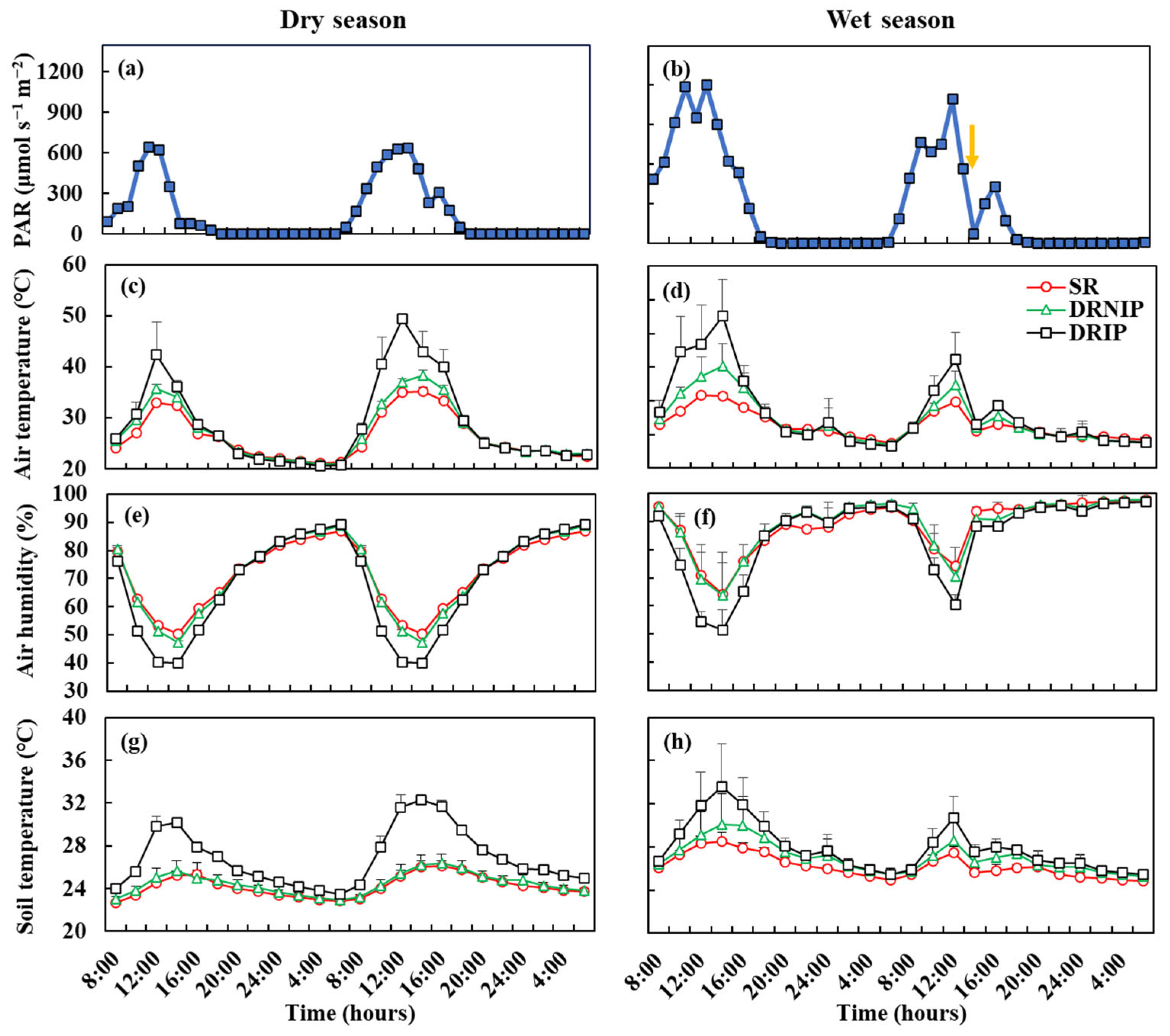
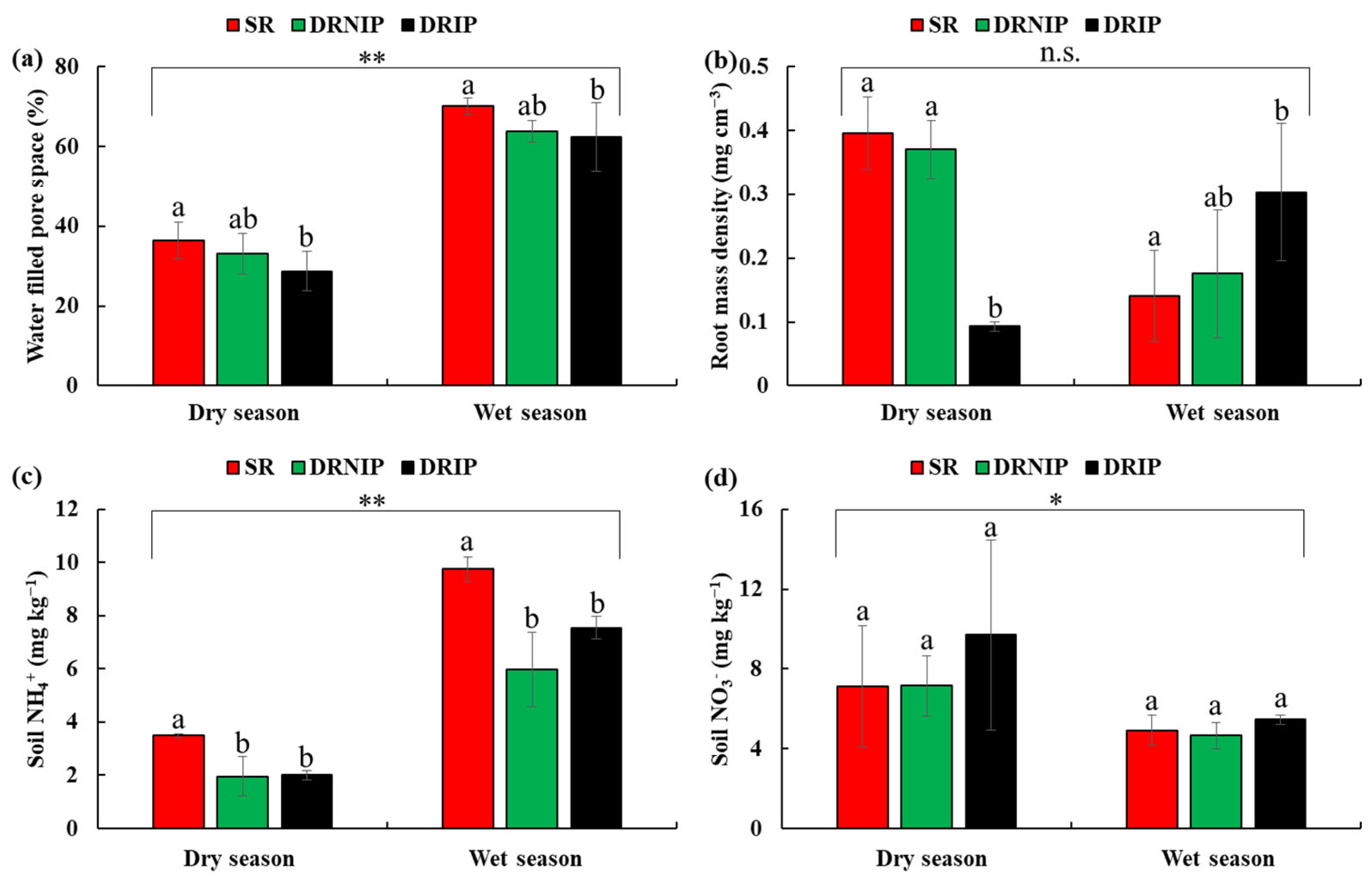
3.1. Environmental Factors

To verify the results and analyze potentially influencing factors, this study measured environmental factors including air temperature, air humidity, soil temperature, soil WFPS, root mass density, and available soil nitrogen content.

During the experimental period, rainfall was recorded in the second 24 h of the wet season, which resulted in a lower PAR (Figure 3b), lower air temperature (Figure 3d), higher air humidity (Figure 3f), and lower soil temperature (Figure 3h). Neglecting the impacts of rainfall, a consistent diurnal pattern was recorded between the dry and wet season among the different plantations. Specifically, the PAR, air temperature, and soil temperature rose around 6:00–8:00 in the morning and gradually decreased after peaking at around 12:00–16:00 in the afternoon (Figure 3e). The air humidity showed an opposite trend, decreasing significantly as the temperature peaked (12:00–14:00), then gradually increasing until peaking in the early morning (2:00–6:00) (Figure 3g). The PAR and air temperature were closest to the daily mean values around 8:00 (and 18:00), and these changed to 9:00 (and 19:00) and 10:00 (and 20:00) for the air humidity and soil temperature, respectively. The average PAR, air temperature, air humidity, and soil temperature in the wet season were 65.95%, 1.16%, 20.75%, and 7.65% higher than that of the dry season, respectively. Additionally, the DRIP represented the highest temperature and lowest humidity among the different treatments in both the dry and wet seasons.

As shown in Figure 4, the non-diurnal environmental factors including WFPS, root mass density, soil NH₄⁺, and soil NO₃⁻ changed a lot from dry to wet seasons. The average WFPS of the different treatments in the dry and wet seasons were 32.74% and 64.37%, respectively, with a significant difference. Compared to the dry season, the root mass densities of SR and DRNIP decreased by 64.37% and 52.57% in the wet season, respectively, while the DRIP increased by more than twice (with significant differences). The total available nitrogen content (the sum of soil NH₄⁺ and NO₃⁻) varied from 9.11–11.70 mg kg⁻¹ and 10.63–14.79 mg kg⁻¹ in the dry and wet seasons, respectively, with no significant difference. Nevertheless, the soil NH₄⁺ and soil NO₃⁻ in the wet season were significantly higher and lower than in the dry season, respectively (Figure 4c,d). Moreover, during the study period (in both seasons), the soil WFPS and NH₄⁺ of the SR were mainly higher than the DRNIP and DRIP, while there was no significant difference in the soil NO₃⁻ among the different treatments.

3.2. Diurnal Variations in Soil Greenhouse Gases

Unlike the diurnal environmental factors that exhibited similar diurnal variation patterns during the study period, the CO₂ and N₂O fluxes showed different patterns between the dry and wet seasons (Figure 5).

In the dry season, the CO₂ fluxes represented continuous fluctuations and similar diurnal variation patterns between the first and second 24 h (varied from 160.13 to 448.92 mg m⁻² h⁻¹), with little distinctions. During the first 24 h, the fluxes among the different treatments showed a similar fluctuating upward trend from the mid-morning (about 8:00–10:00) of the first day to the early morning (2:00–4:00) of the second day, and then a fluctuating downward trend was recorded until the next mid-morning. During the second 24 h, similar CO₂ diurnal emission patterns were recorded, except for a more pronounced and consistent emission peak around 14:00 (Figure 5a).

In the wet season, the CO₂ fluxes also fluctuated continuously during the first 24 h (varied from 175.03 to 726.75 mg m⁻² h⁻¹), but most peaked during daytime hours (about 16:00–18:00) instead of night-time hours compared with the dry season (Figure 5b). Therein, the DRIP had a significantly higher emission peak, while the other treatments experienced relatively stable fluctuations throughout the 24 h. Then, the emission fluxes (varied from 74.84 to 545.80 mg m⁻² h⁻¹) significantly decreased within 2 h after the rainfall, and then showed a fluctuating upward trend in the following 2–8 h. Nevertheless, the daily mean CO₂ fluxes of the second 24 h were slightly lower than the first 24 h among the different treatments.

During the dry season, the daily mean CO₂ flux of SR was significantly higher than that of DRNIP and DRIP, while the situation became the opposite during the wet season (Figure 5c). Such changes were consistent with the root mass density during the study periods (Figure 4b). On average, the emission flux during the wet season was significantly higher than that of the dry season, with the DRIP increasing the most (+83.55%), followed by DRNIP (+34.76%), and SR changing less (+7.11%).

Compared to CO₂, the diurnal variation patterns of N₂O were clearer and more similar among the different treatments (Figure 6). During the consecutive 48 h of dry season, a clear peak at night-time (about 2:00–4:00) was recorded (ranged from 4.05 to 54.11 μg m⁻² h⁻¹), while the first 24 h of the wet season (ranged from 37.82 to 235.87 μg m⁻² h⁻¹) represented a noticeable peak during the daytime (around 14:00). Meanwhile, the N₂O flux in the wet season fluctuated less than the dry season, including all the plantation types. The N₂O emissions in the second 24 h of the wet season were also influenced by the rainfall, with a wider range of variation varying from 27.38 to 259.93 μg m⁻² h⁻¹. Compared to the dry season, the N₂O emissions among all the treatments increased significantly (more than 3 times) in the wet season. Moreover, the DRNIP in the wet season had higher N₂O fluxes than that of the SR and DRIP, with significant differences.

In addition, the results indicated consistent ranges and diurnal variations in GHG fluxes under two replicates, making this an important consideration when collecting GHG samples.

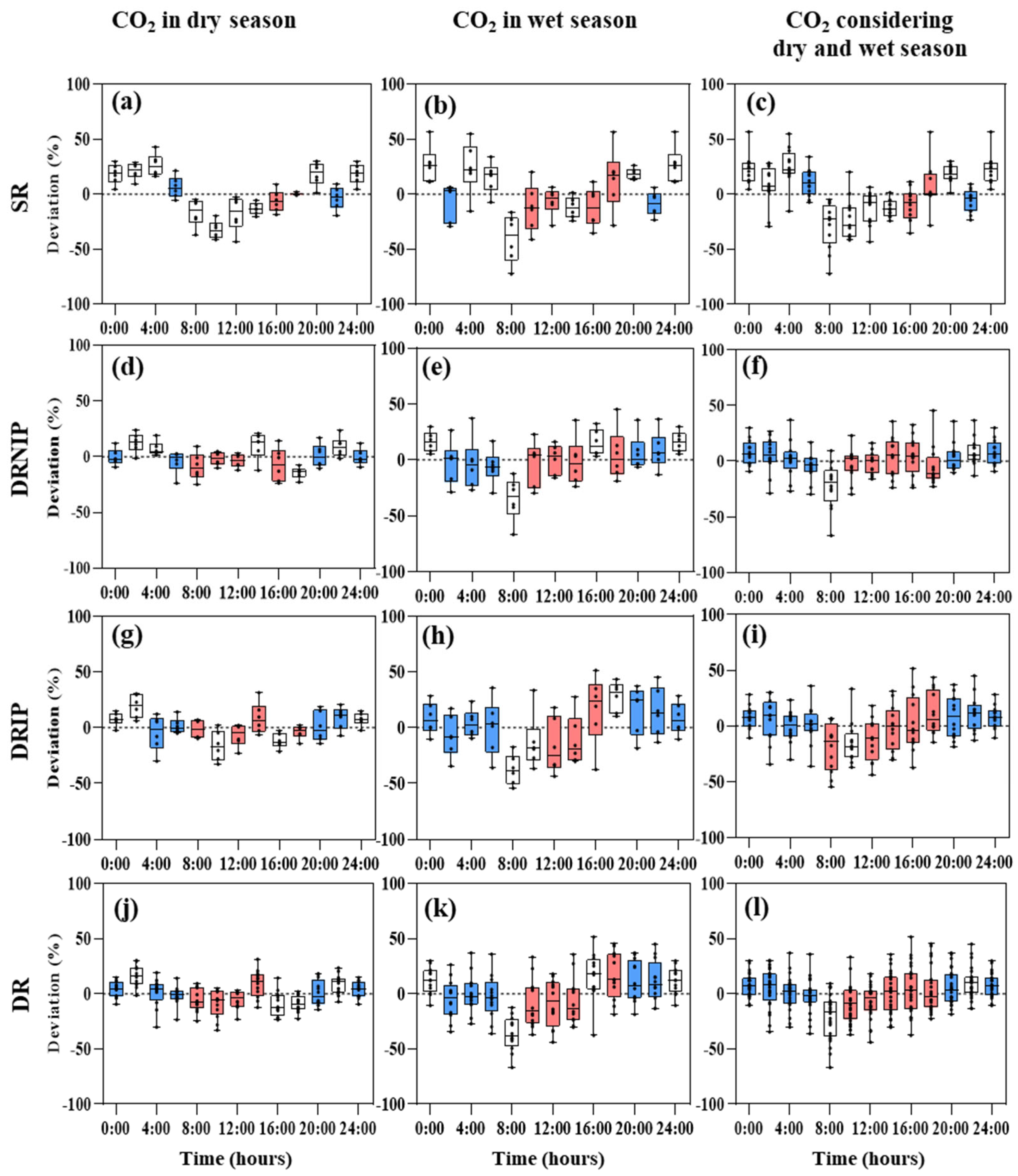
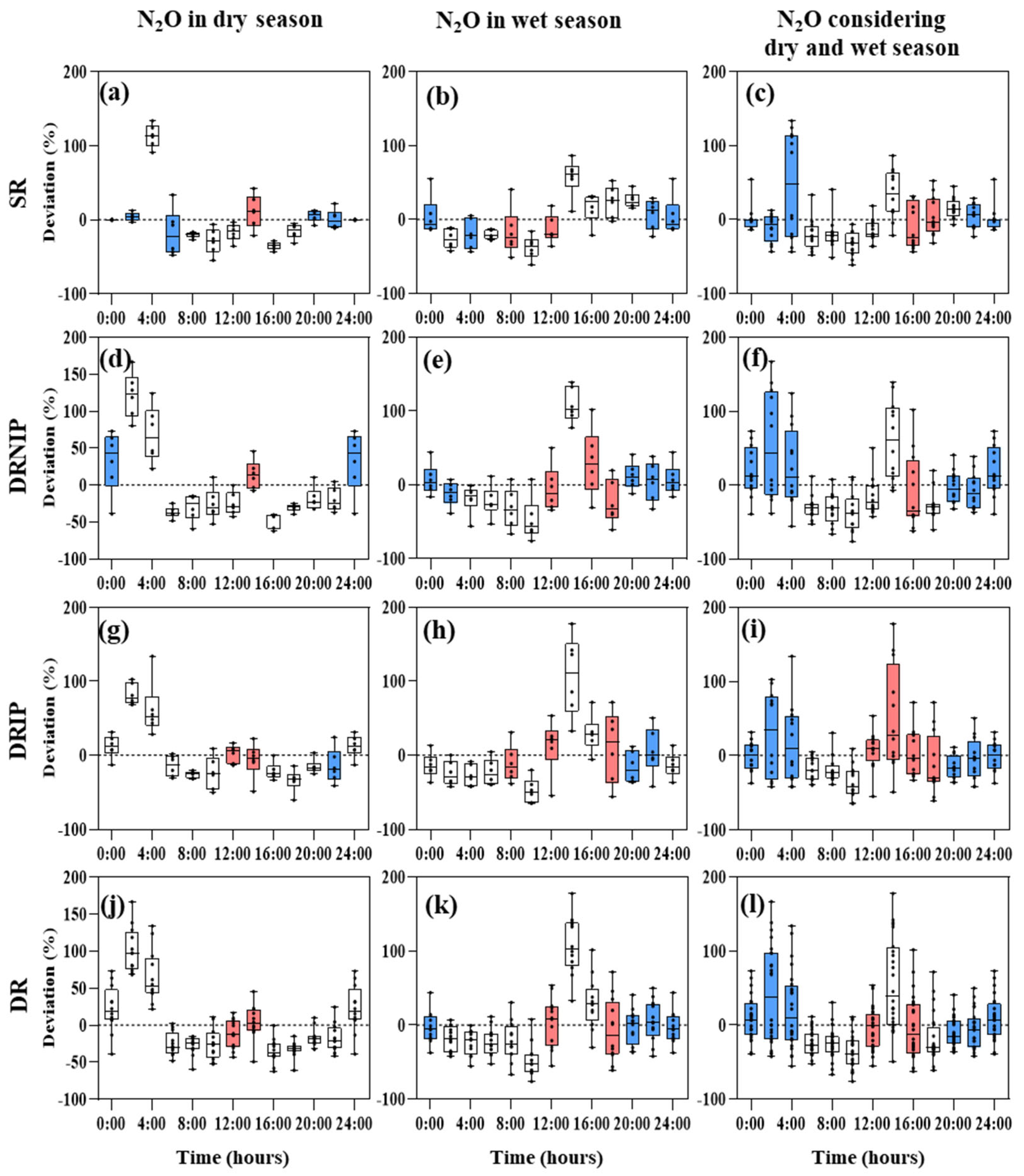
3.3. Suitable Soil Greenhouse Gas Sampling Times

Considering the data representativeness and availability, this study used the data from the consecutive 48 h of the dry season and only the first 24 h of the wet season to determine potentially suitable soil GHG sampling times. The diurnal variations of the deviation between real-time GHG fluxes and daily mean values under different treatments and seasons are depicted in Figure 7 and Figure 8, with deviations closest to zero resembling a more representative sampling time.

The common characteristics of CO₂ and N₂O emissions in all seasons and plantations were that the deviations in the dry season (−32.72%~+26.40% for CO₂ and −40.34%~+140.51% for N₂O) were generally smaller than those in the wet season (−40.41%~+27.67% for CO₂ and −51.94%~+146.12% for N₂O), sampling in the morning times (8:00–10:00) was more likely to cause underestimation (about 25% on average), and the DR (or CO₂) had more potential suitable sampling time intervals than the SR (or N₂O).

The specific situations varied depending on different GHGs, seasons, and treatments. For the CO₂ emitted from the SR treatment, the dry season (or wet season) had a smaller deviations of −6.44% (−12.04%) and −3.76% (−8.67%) around 16:00 and 22:00, respectively. Although the situations with DR were more complex, it could be found that 12:00 was a more suitable sampling time of CO₂ in both dry and wet seasons, and it was strongly recommended to avoid sampling in the morning times (around 8:00) of the wet season.

For the N₂O of SR, the results indicated that only sampling around 22:00 to 24:00 was suitable for both dry and wet seasons, and when considering both dry and wet seasons, it was recommended to sample around 16:00 to 18:00 during the daytime (22:00–4:00 during the night-time). The N₂O sampling of DR (including DRNIP and DRIP) around 14:00 was suggested in the dry season, while it overestimated the fluxes by 50.28% in the wet season. The more recommended sampling times for the wet season were 12:00 and 18:00–22:00. Considering both the dry season and wet season, the results suggested that 16:00 and 20:00–4:00 could be compromised sampling times of N₂O in the DR.

In this study, the results indicated that there were more potential sampling times for CO₂ emissions, the wet season, and improved double-row rubber plantation rather than N₂O emissions, the dry season, and conventional single-row rubber plantation. GHG sampling times should be determined based on these specific situations. The commonly used sampling times in the morning were not suggested in rubber plantations due to the generally consistent and significant underestimation.

3.4. Correlations between Fluxes and Environmental Factors

The correlation analysis indicated that the response of different GHGs to diurnal environmental factors was consistent, and they exhibited opposite trends between the dry and wet seasons (Figure 9). Specifically, in the dry season, both CO₂ and N₂O fluxes positively correlated with air humidity and negatively correlated with air and soil temperature. On the contrary, the fluxes were positively correlated with temperature (including air and soil) and negatively correlated with air humidity in the wet season. Overall, two significant positive correlations were observed in this study, including the GHG fluxes and air humidity in the dry season, as well as the GHG fluxes and temperature (especially soil temperature) in the wet season.

4. Discussion

The diurnal variations in GHGs are a common phenomenon [26,27], which is no exception in this study (Figure 5 and Figure 6). At the same time, there are differences in the diurnal variation patterns of different seasons, GHGs, and treatments. The soil GHG emissions may be influenced by multiple environmental factors and therefore exhibit a large range of diurnal variations. We considered that PAR, air temperature, and soil temperature have similar diurnal patterns, and the soil temperature has a more direct impact on GHG emissions. The following discussion will focus on soil temperature and air humidity (Figure 3), combined with non-diurnal environmental factors between the dry and wet seasons (Figure 4), to analyze their impacts on GHG emissions.

Firstly, the time when the maximum appeared was found to be between the GHG fluxes and soil temperature (and air humidity), especially for the N₂O. In this study, the PAR, air temperature, and soil temperature all reached their peaks around 14:00 in the daytime, while air humidity reached its peak around 2:00 in the nighttime. These phenomena were closely related to the peak of GHGs. Almost all the treatments exhibited significant emission peaks of CO₂ and N₂O during the dry season at night (2:00–4:00), accompanied by a weaker emission peak around 14:00 during the day. During the wet season, the peaks of GHGs were more likely to occur during the day. Also, the correlation analysis illustrated that the air humidity during the dry season and the soil temperature during the wet season were positively correlated with the GHG emissions during the corresponding seasons (Figure 9). These results indicate that the soil temperature and air humidity are important factors influencing the diurnal variation patterns of GHGs.

Secondly, a large number of studies have found that the higher temperature increases GHG emissions (usually peaking around 14:00) by promoting litter decomposition, nitrogen mineralization, microbial activity, etc., and a positive correlation between the two has been recorded [21,24,32]. Wu et al. [26] systematically analyzed 286 N₂O emission datasets and found that 60% of the diurnal variation patterns were significantly correlated with soil temperature, while 20% observed non-diurnal variation patterns without significant temperature correlation. It has been determined that temperature can become one of the dominant factors affecting GHG emissions when the substrate (soil NO₃⁻ and NH₄⁺) and moisture contents are sufficient, thereby allowing for the observation of diurnal variations [21,22]. In this study, a significant positive correlation was recorded between GHGs with temperature during the wet season when soil WFPS was higher (64.37% on average), rather than during the dry season (average soil WFPS was 32.74%), which confirms the above statement.

Thirdly, humidity is also considered to significantly affect GHG emissions over a longer period (e.g., seasonal and annual), and it is usually recorded in the form of rainfall [33,34]. However, the relationship between GHGs and humidity in a diurnal variation is rarely observed, and even if it is, a direct positive correlation has not been found in most cases due to the complex mechanisms of GHG emissions or the uncertainty of monitoring diurnal variations in soil humidity [30]. This study indicated a significant positive correlation between GHG emissions and air humidity during the dry season. The lower soil temperature and WFPS (compared with the wet season), and moderate air humidity (nearly 90% at night) during the dry season (Figure 3) could be an explanation for the reduced sensitivity of GHG to temperature and increased sensitivity to humidity. Ravi et al. [35] indicated that the moisture content of the topsoil layer was significantly affected by air humidity, especially in arid circumstances. Lakhal and Ayyoub [36] demonstrated a similar diurnal variation between soil water content and air humidity. These results indicate that it is possible for soil to harvest moisture from the air, especially in situations where the land is dry but has high air humidity. Therefore, it is reasonable to speculate that the lower soil humidity is influenced by the higher air humidity (especially during the night-time hours of the dry season), leading to alterations in soil GHG emissions despite the slight variations.

In addition, both the CO₂ and N₂O fluxes during the dry season and CO₂ during the wet seasons fluctuated frequently, and such frequent fluctuations have also been found in other studies [37]. It is precisely the multiple factors that contribute to the emissions of soil GHGs, and the limiting factors in different situations may vary [21,26]. One potential reason could be that during the wet season, there is more sufficient moisture and substrate, resulting in a larger emission magnitude and therefore smaller errors in static-chamber sampling. Second, temperature and humidity may have a synergistic effect on the emissions of GHGs in these situations; for example, temperature and humidity are dominant during the daytime and night-time hours, respectively. Additionally, other factors such as the root mass densities cannot be ruled out. In this study, the root mass densities (Figure 4b) and daily mean CO₂ fluxes (Figure 5c) of different treatments showed consistent changes from the dry season to the wet season, which highlighted the importance of roots in soil respiration in rubber plantations, as described by Wu et al. [38]. Also, this study coincidentally recorded a heavy rainfall event in the wet season and its strong interference with soil GHG diurnal variations. Considering the increasing probability of heavy rainfall under the background of climate change and its strong impact on soil GHG emissions [39], future research should focus on the changing diurnal variations in GHG emissions in this context, as well as suitable sampling times.

For suitable sampling times, some studies have recommended morning sampling times for young exotic pine plantations [40], cropland [22], sugarcane cropping systems [23], and tropical forests [25]. Other studies have argued that morning sampling can both overestimate [41] and underestimate [42] the daily mean flux in GHGs. In this study, the results indicated that morning samplings (8:00–10:00) likely resulted in underestimation among all the seasons, GHGs, and plantations (about −25% on average), which could potentially have an impact on the formulation of emission reduction policies. Considering the diversities of the diurnal variations and suitable sampling times, this study suggests that the sampling of soil GHGs in rubber plantations should avoid this clear and consistent underestimation. A suitable sampling time could be 16:00–18:00 to obtain lower deviations from daily mean fluxes in most situations. Nevertheless, there were more potential sampling times for CO₂ emissions, the wet season, and improved double-row rubber plantation rather than N₂O emissions, the dry season, and conventional single-row rubber plantation (Figure 7 and Figure 8). In other words, suitable sampling times could also be diverse, just like the diurnal variations, and suitable GHG sampling times should be determined based on these specific situations.

Future research needs to focus on the diurnal variation patterns over longer periods and other types of rubber-based agroforestry systems with respect for the significant impact of short-term rainfall. Also, it should be pointed out that the emissions and related environmental factors of SR and DR systems vary greatly, especially during the wet season. Therefore, we believe that before promoting DR-based agroforestry systems more reasonably, full consideration should be given to the balance between their comprehensive productivity and carbon costs (or their comprehensive ability to cope with climate stress), with full respect for soil GHG emissions because of their important role.

5. Conclusions

Developing rubber-based agroforestry systems could be one of the potential ways for rubber plantation and agricultural production in tropical regions to address ecosystem services including climate mitigation. For increasing the accuracy of GHG estimation, it is a crucial step to understand the diurnal variations and suitable sampling times for the manual static chamber method. In this study, the diurnal variation patterns of CO₂ in rubber plantations were likely to remain fluctuating, with the maximum flux typically occurring during the night-time and daytime hours of the dry season and wet season, respectively. A clearer double-peak (around 2:00 and 14:00) during the dry season and a daytime peak (14:00) during the wet season of the N₂O were recorded. The sampling of soil GHGs in rubber plantations should be conducted during the late afternoon (16:00–18:00) instead of the most common morning times (underestimation of 25% on average). In addition to the commonalities, different seasons and different types of GHGs and rubber plantations also differed in their detailed fluctuation times and ranges, and therefore the determination of suitable sampling times should not ignore these factors in certain cases. Additionally, the air humidity during the dry season and the soil temperature during the wet season were both positively correlated with GHGs (p < 0.05). This study provides a resource for decreasing the bias of GHG estimation of rubber-based agroforestry in Hainan Island, China.

References

1. AR6 Synthesis Report: Climate Change 2023. Available online: https://www.ipcc.ch/report/sixth-assessment-report-cycle/ (accessed on 31 December 2023).
2. AR5 Synthesis Report: Climate Change 2014. Available online: https://www.ipcc.ch/report/ar5/syr/ (accessed on 31 December 2023).
3. Lal, R. Farming systems to return land for nature: It’s all about soil health and re-carbonization of the terrestrial biosphere. Farm. Syst. 2023, 1, 100002. [Google Scholar] [CrossRef]
4. Paustian, K.; Lehmann, J.; Ogle, S.; Reay, D.; Robertson, G.P.; Smith, P. Climate-smart soils. Nature 2016, 532, 49–57. [Google Scholar] [CrossRef]
5. Tian, H.; Lu, C.; Ciais, P.; Michalak, A.M.; Canadell, J.G.; Saikawa, E.; Huntzinger, D.N.; Gurney, K.R.; Sitch, S.; Zhang, B.; et al. The terrestrial biosphere as a net source of greenhouse gases to the atmosphere. Nature 2016, 531, 225–228. [Google Scholar] [CrossRef] [PubMed]
6. Kumar, A.; Kumar, A.; Kumar, M.; Bhat, J.A. Editorial: Greenhouse gas emissions and terrestrial ecosystems. Front. Environ. Sci. 2022, 10, 834444. [Google Scholar] [CrossRef]
7. Singh, A.K.; Liu, W.; Zakari, S.; Wu, J.; Yang, B.; Jiang, X.J.; Zhu, X.; Zou, X.; Zhang, W.; Chen, C.; et al. A global review of rubber plantations: Impacts on ecosystem functions, mitigations, future directions, and policies for sustainable cultivation. Sci. Total Environ. 2021, 796, 148948. [Google Scholar] [CrossRef]
8. Qi, D.; Wu, Z.; Yang, C.; Xie, G.; Li, Z.; Yang, X.; Li, D. Can intercropping with native trees enhance structural stability in young rubber (Hevea brasiliensis) agroforestry system? Eur. J. Agron. 2021, 130, 126353. [Google Scholar] [CrossRef]
9. Chen, C.; Liu, W.; Wu, J.; Jiang, X.; Zhu, X. Can intercropping with the cash crop help improve the soil physico-chemical properties of rubber plantations? Geoderma 2019, 335, 149–160. [Google Scholar] [CrossRef]
10. Rodrigo, V.H.L.; Silva, T.U.K.; Munasinghe, E.S. Improving the spatial arrangement of planting rubber (Hevea brasiliensis Muell. Arg.) For long-term intercropping. Field Crops Res. 2004, 89, 327–335. [Google Scholar] [CrossRef]
11. Jessy, M.D.; Shankar, M.; Nair, N.U. A cropping system for reduction of gestation period and enhanced yield of rubber trees (Hevea brasiliensis). Rubber Sci. 2013, 26, 210–216. [Google Scholar]
12. Oliosi, G.; Oliveira, M.G.; Partelli, F.L. Microclimate and development of black pepper intercropped with rubber tree. Agrofor. Syst. 2021, 95, 1635–1645. [Google Scholar] [CrossRef]
13. FAOATAT. Available online: https://www.fao.org/faostat/en/#data (accessed on 31 December 2022).
14. Zeng, X.; Cai, M.; Lin, W. Improving planting pattern for intercropping in the whole production span of rubber tree. Afr. J. Biotechnol. 2012, 11, 8484–8490. [Google Scholar] [CrossRef]
15. Zhou, L.; Lin, W.; Zeng, X.; Cai, M.; Chen, J.; Huang, J.; Pan, J.; Zheng, D.; Zhou, J. Investigation on a new rubber based farming system in China. In Proceedings of the CRRI and IRRDB International Rubber Conference, Siem Reap, Cambodia, 24–25 November 2016. [Google Scholar]
16. Huang, J.; Pan, J.; Zhou, L.; Zheng, D.; Yuan, S.; Chen, J.; Li, J.; Gui, Q.; Lin, W. An improved double-row rubber (Hevea brasiliensis) plantation system increases land use efficiency by allowing intercropping with yam bean, common bean, soybean, peanut, and coffee: A 17-year case study on Hainan island, China. J. Clean. Prod. 2020, 263, 121493. [Google Scholar] [CrossRef]
17. Dong, T. Response of Intercropped Ficus Hirta Vahl Growth and Yield to Nitrogen Fertilization in Different Rubber Plantations; China Agricultural University: Beijing, China, 2023. (In Chinese) [Google Scholar]
18. Rao, X.; Liu, C.; Tang, J.; Nie, Y.; Liang, M.; Shen, W.; Siddique, K.H.M. Rubber-leguminous shrub systems stimulate soil N2O but reduce CO2 and CH4 emissions. For. Ecol. Manag. 2021, 480, 118665. [Google Scholar] [CrossRef]
19. Tang, X.; Liu, S.; Zhou, G.; Zhang, D.; Zhou, C. Soil-atmospheric exchange of CO2, CH4, and N2O in three subtropical forest ecosystems in southern China. Glob. Chang. Biol. 2006, 12, 546–560. [Google Scholar] [CrossRef]
20. Wang, Y.; Wang, Y. Quick measurement of CH4, CO2 and N2O emissions from a short-plant ecosystem. Adv. Atmos. Sci. 2003, 20, 842–844. [Google Scholar]
21. Reeves, S.; Wang, W. Optimum sampling time and frequency for measuring N2O emissions from a rain-fed cereal cropping system. Sci. Total Environ. 2015, 530–531, 219–226. [Google Scholar] [CrossRef] [PubMed]
22. Alves, B.J.R.; Smith, K.A.; Flores, R.A.; Cardoso, A.S.; Oliveira, W.R.D.; Jantalia, C.P.; Urquiaga, S.; Boddey, R.M. Selection of the most suitable sampling time for static chambers for the estimation of daily mean N2O flux from soils. Soil. Biol. Biochem. 2012, 46, 129–135. [Google Scholar] [CrossRef]
23. Reeves, S.; Wang, W.; Salter, B.; Halpin, N. Quantifying nitrous oxide emissions from sugarcane cropping systems: Optimum sampling time and frequency. Atmos. Environ. 2016, 136, 123–133. [Google Scholar] [CrossRef]
24. Cueva, A.; Bullock, S.H.; López-Reyes, E.; Vargas, R. Potential bias of daily soil CO2 efflux estimates due to sampling time. Sci. Rep. 2017, 7, 11925. [Google Scholar] [CrossRef]
25. Yang, H.; Liu, S.; Li, Y.; Xu, H. Diurnal variations and gap effects of soil CO2, N2O and CH4 fluxes in a typical tropical montane rainforest in Hainan island, China. Ecol. Res. 2018, 33, 379–392. [Google Scholar] [CrossRef]
26. Wu, Y.; Whitaker, J.; Toet, S.; Bradley, A.; Davies, C.A.; Mcnamara, N.P. Diurnal variability in soil nitrous oxide emissions is a widespread phenomenon. Glob. Chang. Biol. 2021, 27, 4950–4966. [Google Scholar] [CrossRef] [PubMed]
27. Lammirato, C.; Wallman, M.; Weslien, P.; Klemedtsson, L.; Rütting, T. Measuring frequency and accuracy of annual nitrous oxide emission estimates. Agric. For. Meteorol. 2021, 310, 108624. [Google Scholar] [CrossRef]
28. Tian, S.; Ning, T.; Chi, S.; Wang, Y.; Wang, B.; Han, H.; Li, C.; Li, Z. Diurnal variations of the greenhouse gases emission and their optimal observation duration under different tillage systems. Acta Ecol. Sin. 2012, 32, 879–888. [Google Scholar] [CrossRef]
29. Wang, X.; Feng, Y.; Yu, L.; Shu, Y.; Tan, F.; Gou, Y.; Luo, S.; Yang, W.; Li, Z.; Wang, J. Sugarcane/soybean intercropping with reduced nitrogen input improves crop productivity and reduces carbon footprint in China. Sci. Total Environ. 2020, 719, 137517. [Google Scholar] [CrossRef] [PubMed]
30. Yu, X.; Li, X.; Xu, L.; Wang, M.; Zhang, J.; Jiang, M.; Wang, G. Diurnal variation of soil CO2 efflux and its optimal measuring time-window of temperate meadow steppes in western Songnen plain, China. Chin. Geogr. Sci. 2020, 26, 518–526. [Google Scholar] [CrossRef]
31. Liu, X.J.; Mosier, A.R.; Halvorson, A.D.; Reule, C.A.; Zhang, F.S. Dinitrogen and N2O emissions in arable soils: Effect of tillage, n source and soil moisture. Soil Biol. Biochem. 2007, 39, 2362–2370. [Google Scholar] [CrossRef]
32. Savage, K.; Phillips, R.; Davidson, E. High temporal frequency measurements of greenhouse gas emissions from soils. Biogeosciences 2014, 11, 2709–2720. [Google Scholar] [CrossRef]
33. Duan, B.; Cai, T.; Man, X.; Xiao, R.; Gao, M.; Ge, Z.; Mencuccini, M. Different variations in soil CO2, CH4, and N2O fluxes and their responses to edaphic factors along a boreal secondary forest successional trajectory. Sci. Total Environ. 2022, 838, 155983. [Google Scholar] [CrossRef]
34. Jovani-Sancho, A.J.; O’Reilly, P.; Anshari, G.; Chong, X.Y.; Crout, N.; Evans, C.D.; Evers, S.; Gan, J.Y.; Gibbins, C.N.; Gusmayanti, E.; et al. CH4 and N2O emissions from smallholder agricultural systems on tropical peatlands in southeast Asia. Glob. Chang. Biol. 2023, 29, 4279–4297. [Google Scholar] [CrossRef]
35. Ravi, S.; D’Odorico, P.; Over, T.M.; Zobeck, T.M. On the effect of air humidity on soil susceptibility to wind erosion: The case of air-dry soils. Geophys. Res. Lett. 2004, 31, L09501. [Google Scholar] [CrossRef]
36. Lakhal, E.; Ayyoub, A. Effect of air relative humidity harvest on soil moisture content under moroccan climatic conditions. J. Eng. Res. Appl. 2015, 4, 74–82. [Google Scholar] [CrossRef]
37. Metya, A.; Datye, A.; Chakraborty, S.; Tiwari, Y.K.; Sarma, D.; Bora, A.; Gogoi, N. Diurnal and seasonal variability of CO2 and CH4 concentration in a semi-urban environment of western India. Sci. Rep. 2021, 11, 2931. [Google Scholar] [CrossRef] [PubMed]
38. Wu, Z.; Guan, L.; Chen, B.; Yang, C.; Lan, G.; Xie, G.; Zhou, Z. Components of soil respiration and its monthly dynamics in rubber plantation ecosystems. In Proceedings of the 2013 Fourth International Conference on Digital Manufacturing & Automation, Qindao, China, 29–30 June 2013; pp. 361–369. [Google Scholar] [CrossRef]
39. Li, L.; Hao, Y.; Zheng, Z.; Wang, W.; Biederman, J.A.; Wang, Y.; Wen, F.; Qian, R.; Xu, C.; Zhang, B.; et al. Heavy rainfall in peak growing season had larger effects on soil nitrogen flux and pool than in the late season in a semiarid grassland. Agric. Ecosyst. Environ. 2022, 326, 107785. [Google Scholar] [CrossRef]
40. Wang, Y.; Wang, H.; Wang, Z.; Zhang, W.; Guo, C.; Wen, X.; Liu, Y. Optimizing manual sampling schedule for estimating annual soil CO2 efflux in a young exotic pine plantation in subtropical China. Eur. J. Soil. Biol. 2012, 52, 41–47. [Google Scholar] [CrossRef]
41. Scheer, C.; Rowlings, D.W.; Firrel, M.; Deuter, P.; Morris, S.; Grace, P.R. Impact of nitrification inhibitor (DMPP) on soil nitrous oxide emissions from an intensive broccoli production system in sub-tropical Australia. Soil Biol. Biochem. 2014, 77, 243–251. [Google Scholar] [CrossRef]
42. Savage, K.E.; Davidson, E.A. A comparison of manual and automated systems for soil CO2 flux measurements: Trade-offs between spatial and temporal resolution. J. Exp. Bot. 2003, 54, 891–899. [Google Scholar] [CrossRef]
Figure 1. Study site of the experiment.
Forests 15 00950 g001
Figure 2. Schematic diagram of the rubber plantations and the location of the greenhouse gas sampling.
Forests 15 00950 g002
Figure 3. Diurnal environmental factors between dry season (a,c,e,g) and wet season (b,d,f,h). (Note: the yellow arrow in the (b) indicates a heavy rainfall (23.2 mm) from 13:40 to 14:20.).
Forests 15 00950 g003
Figure 4. Non-diurnal environmental factors in different rubber plantations during the study period. (a) water filled pore space; (b) root mass density of rubber trees; (c) soil NH4+ content; (d) soil NO3 content. Values in the bar chart are the mean ± SD. Different lowercase letters represent significant differences among different treatments (LSD, p < 0.05); * p  <  0.05, ** p  <  0.01, and n.s. as not significant.
Forests 15 00950 g004
Figure 5. Diurnal variations (a,b) and average fluxes (c) of CO2 in different plantations. Error bars in line charts indicate + SD (n = 3). Values in the bar chart are the mean ± SD (n = 6). Different lowercase letters represent significant differences among different breakdowns (LSD, p < 0.05); * p  <  0.05.
Forests 15 00950 g005
Figure 6. Diurnal variations (a,b) and average fluxes (c) of N2O in different plantations. Error bars in line charts indicate + SD (n = 3). Values in the bar chart are the mean ± SD (n = 6). Different lowercase letters represent significant differences among different breakdowns (LSD, p < 0.05); ** p  <  0.01.
Forests 15 00950 g006
Figure 7. Soil CO2 emission flux deviations from daily averages in the dry season (a,d,g,j), wet season (b,e,h,k), and both of them (c,f,i,l). Red boxes and blue boxes represent potentially suitable sampling times during daytime (8:00–18:00) and night-time (20:00–6:00), respectively. The center lines of each boxplot show the medians, box limits indicate the 25th and 75th percentiles, and whiskers extend to the minimal and maximal values, as determined using GraphPad Prism 8.0.1 software.
Forests 15 00950 g007
Figure 8. Soil N2O emission flux deviations from daily averages in the dry season (a,d,g,j), wet season (b,e,h,k), and both of them (c,f,i,l). Red boxes and blue boxes represent potentially suitable sampling times during daytime (8:00–18:00) and night-time (20:00–6:00), respectively. The center lines of each boxplot show the medians, box limits indicate the 25th and 75th percentiles, and whiskers extend to the minimal and maximal values, as determined using GraphPad Prism 8.0.1 software.
Forests 15 00950 g008
Figure 9. Relationships between GHG fluxes and diurnal environmental factors in different seasons. CO2 and air temperature (a), air humidity (b), and soil temperature (c); N2O and air temperature (d), air humidity (e), and soil temperature (f). Linear regression using averages of two days in the dry season and the first day in the wet season (n = 216). Statistical significance is calculated as ** p  <  0.01, and n.s. as not significant.
Forests 15 00950 g009
Disclaimer/Publisher’s Note: The statements, opinions and data contained in all publications are solely those of the individual author(s) and contributor(s) and not of MDPI and/or the editor(s). MDPI and/or the editor(s) disclaim responsibility for any injury to people or property resulting from any ideas, methods, instructions or products referred to in the content.