Article

Cunninghamia lanceolata Canopy Relative Chlorophyll Content Estimation Based on Unmanned Aerial Vehicle Multispectral Imagery and Terrain Suitability Analysis

1
College of Forestry, Fujian Agriculture and Forestry University, Fuzhou 350028, China
2
University Key Lab for Geomatics Technology and Optimized Resources Utilization in Fujian Province, Fuzhou 350002, China
*
Author to whom correspondence should be addressed.
Forests 2024, 15(6), 965; https://doi.org/10.3390/f15060965
Submission received: 14 April 2024 / Revised: 27 May 2024 / Accepted: 28 May 2024 / Published: 31 May 2024
(This article belongs to the Special Issue UAV Application in Forestry)

Abstract

:
This study aimed to streamline the determination of chlorophyll content in Cunninghamia lanceolate while achieving precise measurements of canopy chlorophyll content. Relative chlorophyll content (SPAD) in the Cunninghamia lanceolate canopy were assessed in the study area using the SPAD-502 portable chlorophyll meter, alongside spectral data collected via onboard multispectral imaging. And based on the unmanned aerial vehicle (UAV) multispectral collection of spectral values in the study area, 21 vegetation indices with significant correlation with Cunninghamia lanceolata canopy SPAD (CCS) were constructed as independent variables of the model’s various regression techniques, including partial least squares regression (PLSR), random forests (RF), and backpropagation neural networks (BPNN), which were employed to develop a SPAD inversion model. The BPNN-based model emerged as the best choice, exhibiting test dataset coefficients of determination (R2) at 0.812, root mean square error (RSME) at 2.607, and relative percent difference (RPD) at 1.942. While the model demonstrated consistent accuracy across different slope locations, generalization was lower for varying slope directions. By creating separate models for different slope directions, R2 went up to about 0.8, showcasing favorable terrain applicability. Therefore, constructing inverse models with different slope directions samples separately can estimate CCS more accurately.

1. Introduction

Chlorophyll serves as the primary pigment essential for photosynthesis within the forest canopy, enabling light absorption to fuel the Calvin cycle [1]. It stands as a key biochemical parameter within this ecosystem. The precise and prompt assessment of chlorophyll content not only aids in evaluating the photosynthetic capacity and physiological well-being of forest trees but also provides insights into their overall health status [2]. This information carries significant implications for estimating terrestrial carbon flux cycles and biomass levels.
Traditional methods for determining chlorophyll content in forest canopies, such as spectrophotometry and fluorescence analysis, are known for their superior accuracy [3,4]. However, these methods entail intricate and cumbersome operations, making sampling challenging and time-consuming while also consuming substantial energy. Moreover, the transportation of leaf blade chlorophyll samples can result in certain losses. In recent years, the handheld chlorophyll meter has gained popularity as a nondestructive and portable tool for assessing relative chlorophyll content (SPAD), which has been widely adopted in chlorophyll content analysis [5,6]. SPAD serves to quantify the greenness of plant leaves, with prior research demonstrating a significant positive correlation between SPAD and chlorophyll content, allowing for highly accurate conversions [1,7]. Despite its advantages, the handheld chlorophyll meter is limited to contact measurements on individual samples, necessitating extensive sampling and limiting the scope of chlorophyll estimation. With ongoing advancements in remote sensing platforms, sensors, and data-processing methodologies, the field of remote sensing has alleviated the shortcomings of traditional survey methods, providing an effective alternative for rapidly and accurately collecting forest parameter data [8,9,10,11].
Among many remote sensing techniques, satellite remote sensing has been favored by many scholars in the estimation of chlorophyll content due to its ability to collect information over a wide range and multiple time phases [11,12,13,14]. However, as satellites fly along fixed orbits, their information collection for an area is cyclical, which makes it difficult for satellite remote sensing to meet the real-time probing of chlorophyll content of forest trees [15]. On the other hand, the lower spatial resolution makes it difficult for satellite remote sensing to focus on the monitoring of the canopy chlorophyll of a single tree, and makes it difficult for the spectral reflectance obtained from its collection to match with the canopy chlorophyll content obtained from ground surveys; thus, it also makes it difficult to match the spectral reflectance collected by satellite remote sensing with the canopy chlorophyll content obtained from ground surveys, thus reducing the accuracy of canopy chlorophyll content determination [16]. Compared with satellite remote sensing, unmanned aerial vehicle (UAV) remote sensing technology can not only meet the needs of large-scale chlorophyll content monitoring, but can also obtain higher-resolution remote sensing images according to the needs of users [17].
UAV remote sensing technology leverages hyperspectral or multispectral sensors to capture spectral images of the target area, enabling the estimation of chlorophyll content. Specifically, UAV hyperspectral technology has demonstrated exceptional accuracy in chlorophyll content estimation within plant canopies, owing to its broad response range and high resolution [18,19,20,21]. However, challenges such as high costs, data redundancy, processing complexity, and restrictive operational conditions have hindered its widespread adoption in practical forestry applications. In the past, multispectral cameras have been widely used for quantitative inversion of plant physiological parameters due to their low cost and practicality. Nevertheless, the spectral resolution of multispectral images is in the range of λ/10 order of magnitude, which is much higher than that of hyperspectral, in the range of λ/100 order of magnitude. As a result, it is more difficult for multispectral imagery to accurately capture changes in forest SPAD than hyperspectral imagery. Previous studies have attempted to enhance the prediction of plant canopy SPAD by modifying the features integrated into modeling [22,23,24] and by exploring and contrasting diverse model construction techniques [25,26,27]. However, factors like geographical region, lighting conditions, image capture elevation, and terrain can impact model construction and predictive performance [28,29]. Among them, terrain includes factors such as elevation, slope directions, and the slope of the forest planting site [30], and the influence of terrain on the construction of large-area models is difficult to control, and the poor applicability of the models to different topographies still exists in the field of remote sensing inversion of forest canopy SPAD, which is worth exploring further.
Cunninghamia lanceolata (Lamb.) Hook has a planted area of 9.90 × 10⁶ hm2 in China, with a volume of 7.55 × 10⁸ m3, ranking first in the total area and volume of planted tree forests in the country [31], and the management of Cunninghamia lanceolata plantation forests is of great significance for timber production and maintenance of ecological functions [32]. The management and management of Cunninghamia lanceolata plantation forests are important in terms of timber production and maintenance of ecological functions. Among them, the judgment and monitoring of the health status of Cunninghamia lanceolata plantation forests is an important means to improve the quality and ecological benefits of Cunninghamia lanceolata plantation forests [33]. As one of the important indexes to measure the growth and health status of Cunninghamia lanceolata, the accuracy and timeliness of the observed values of the chlorophyll content are of great significance to the management of Cunninghamia lanceolata and even to the country to guarantee the quality of timber and ecological safety.
In this study, the focus is on Cunninghamia lanceolata plantation forests, where a Cunninghamia lanceolata canopy SPAD (CCS) inversion model is established utilizing UAV multispectral imagery. The model aims to identify and select appropriate vegetation indices as independent variables, compare prediction performance across different modeling methods, and evaluate model applicability from a terrain perspective. The primary objective is to realize the accurate measurement of CCS in a wide range, and provide theoretical basis and technical support for the growth monitoring and health evaluation of Cunninghamia lanceolata.

2. Materials and Methods

2.1. Study Areas

The study area is situated within the state-owned forest region of Shunchang County, Nanping City, Fujian Province, China, and spanning longitudes 117°9′ to 118°4′ and latitudes 26°8′ to 27°21′. Encompassing a length of 74 km east to west and a width of 61 km north to south, the area experiences a humid monsoon climate characteristic of the central subtropical zone. Abundant rainfall and sunshine define the climatic conditions, with an average annual temperature of 19.2 °C and a frost-free period lasting 289 days. The average annual precipitation measures 2144 mm. The forested land boasts a deep and ample soil layer predominantly composed of red loam soil, with minimal barren soil patches. Forested areas dominate and exhibit high coverage rates, indicative of preferable forest quality. Spanning a total land area of 23,799.20 hm2, the region features 161.95 m3/hm2 of Cunninghamia lanceolata storage. Coniferous forests prevail as the predominant tree type, occupying 10,852.70 hectares with a storage capacity of 1,295,718 m3. These coniferous forests account for 46.39% of the total woodland area and 43.76% of the total forest area storage capacity in the region [34].
The study area is a Cunninghamia lanceolata plantation near-mature pure forest with a degree of depression of 0.7, a slope gradient of 30°, and slope lengths all greater than 60 m. The soil is a Class I fertile red loam, and the forest management type is general Cunninghamia lanceolata medium-diameter timber. In this study, based on the dichotomy of slope directions, the slope directions were divided into sunny and shady slope directions by using small-group contour maps combined with the use of a compass in the field [35] (Figure 1), and, at the same time, the slopes were equally divided into upper and lower parts. In addition, since most Cunninghamia lanceolata plantation forests in southern China are planted in hilly terrain, and elevation differences between hills are small, the elevation factor in terrain factors was not included in the discussion in this study.

2.2. Data Collection

2.2.1. Measurement of CCS

In March 2023, 270 Cunninghamia lanceolata samples were randomly selected from sample plots with different slope directions and slope locations in the Cunninghamia lan-ceolata plantation near-mature forest stand in Shunchang County, Nanping City, Fujian Province, China, and the distribution of the samples is shown in Figure 2. The sample canopy was divided into upper, middle, and lower layers, and within each layer, a number of unobstructed branches were cut from each layer using a tall branch shear with a pole length of 10 m. From the cut branches, 10–20 leaves were randomly selected, and the SPAD values of the selected leaves were measured immediately using a handheld chlorophyll meter (SPAD-502, Konica Minolta, Tokyo, Japan), and the average value of each leaf was calculated by taking 3 measurements at different parts of each leaf, and finally, 5 leaves were counted. The measured CCS for the upper location of sunny slope (USunny), the lower location of sunny slope (LSunny), the upper location of shady slope (UShady), and the lower location of shady slope (LShady) is shown in Figure 3.

2.2.2. Collection and Processing of UAV Imagery

A quadcopter mini UAV, DJI Phantom 4 equipped with a multispectral sensor, was used to collect remote sensing images of the Cunninghamia lanceolata artificial forest area. The camera can capture spectral images in five different spectral channels simultaneously. The five 2.08-megapixel monochrome sensors cover the following spectral bands: blue (450 nm ± 16 nm), green (560 nm ± 16 nm), red (650 nm ± 16 nm), red-edge (730 nm ± 16 nm), and near-infrared (840 nm ± 26 nm).
In order to reduce the influence of shadows and solar light intensity on the inversion results, the cloudy and maximum solar altitude angle time period was selected for aerial photography operations. Based on previous studies combined with elevation and average stand height in the study area [29,36], the DJI Wizard P4 multispectral version was set to have a route altitude of 80 m, an overlap rate of 85% in the heading direction, an overlap rate of 80% in the side direction, and a gimbal pitch angle of 90°, and a route design of 90° was carried out based on the target area of the small-class. route design for semi-automatic aerial photography by UAV. After the remote sensing images were collected, DJI and ENVI 5.3 software were used to correct the radiation and remove the noise from the multispectral images.

2.3. Data Processing

2.3.1. Selection of Vegetation Indices

The spectral characteristics of green plant leaves and vegetation canopy, as well as their differences and changes, can reflect the vegetation information on remote sensing images. However, the spectral reflectance of forest vegetation is susceptible to the influence of various factors such as the ground, the atmosphere, the canopy structure, etc. [37,38], while the vegetation index can weaken the influence of external factors, enhance the sensitivity to changes in vegetation, and can quickly, simply, and efficiently measure the health of the vegetation growth and the coverage of the vegetation. Drawing on previous research and the spectral features of chlorophyll, this study employed ENVI 5.3 software to calculate 21 vegetation indices from the five monochrome spectral images collected by the UAV. The formulas for these 21 vegetation indices are presented in Table 1. The relationship between each vegetation index and measured CCS was analyzed using SPSS 25, and the vegetation indices with significant correlations with CCS were screened as independent variables to participate in the CCS inversion modeling.
In order to reduce the influence of background values on the vegetation index of the samples, this study constructed circular buffers with a radius of 0.5 m for each sample centered on the tree apex based on the canopy size measured in the field. The mean of the pixel values of each buffer was then extracted as the vegetation index value of each sample using ArcGIS 10.8.

2.3.2. Model Establishment

In this study, using the Python 3.7 software platform, three modeling methods were selected: partial least squares regression (PLSR), random forest regression (RF), and backpropagation neural networks (BPNN). Three vegetation indices with the highest correlation to the CCS were chosen as independent variables, while the measured SPAD served as the dependent variable for constructing the inversion model.
Previous studies have shown that the estimation models constructed by combinations of different vegetation indices have higher estimation accuracy and performance than single-band, single-variable estimation models [23]. However, the multicollinearity among the vegetation indices weakened their explanatory power for the estimation indexes. Therefore, in this study, PLSR was selected to build a linear estimation model of CCS, aiming at weakening the high correlation among the independent variables [55]. RF, on the other hand, as one of the most representative of the integration algorithms, is able to provide an assessment of the importance of each feature, which helps to understand which features contribute the most to the model. This ability of feature selection makes random forests more convenient in dealing with features of different scales, which demonstrates its powerful performance in a variety of realistic tasks [56,57]. BPNN, as one of the most widely used neural networks, has a powerful nonlinear mapping ability, which allows it to approximate any complex nonlinear function through a multilayer network structure. This makes BP neural networks have higher accuracy and stronger generalization ability when dealing with data with complex nonlinear relationships [58]. However, in the construction of the BPNN model, too many input nodes not only increase the training time cost of the model, but also may cause the neural network to be too sensitive to the noise and redundant information in the input vectors, which reduces the generalization ability and prediction accuracy of the model. In order to avoid the above problems, principal component analysis (PCA) was used in this study for dimensionality reduction of the input data.

2.3.3. Accuracy Evaluation

After removing some outliers, the remaining 255 samples are divided into a training dataset with a sample size of 200 as well as a test dataset of 55 in the ratio of 8:2, while 25% of the samples from the training dataset are randomly selected for the test of model training performance. The performance and accuracy of the model were comprehensively compared using the model’s coefficient of determination (R2), root mean square error (RMSE), and relative percent difference (RPD). A higher R2 closer to 1 during inversion modeling and test indicates higher estimation accuracy of the model. Similarly, a lower RMSE suggests better predictive performance, indicating smaller differences between predicted and observed values. For the evaluation criteria of RPD: when RPD < 1.4, the model is considered unable to predict the samples effectively; when 1.4 < RPD < 2, the model demonstrates good predictive capability for the samples; and when RPD > 2, the model exhibits strong sample prediction ability. The formulas for evaluating model accuracy are as follows:
R 2 = 1 i = 1 n y i y ^ i 2 i = 1 n y i y ¯ i 2
R M S E = 1 n i = 1 n y i y ^ i 2
S D = 1 n 1 i = 1 n y ^ i y ¯ i 2
R P D = S D R M S E
where the n is the number of samples, i is the sample ordinal number, y i is the measured value of CCS, y ^ i is the predicted value of CCS, y ¯ i is the mean of the measured value of CCS, and SD is the standard deviation of the model prediction.

3. Results

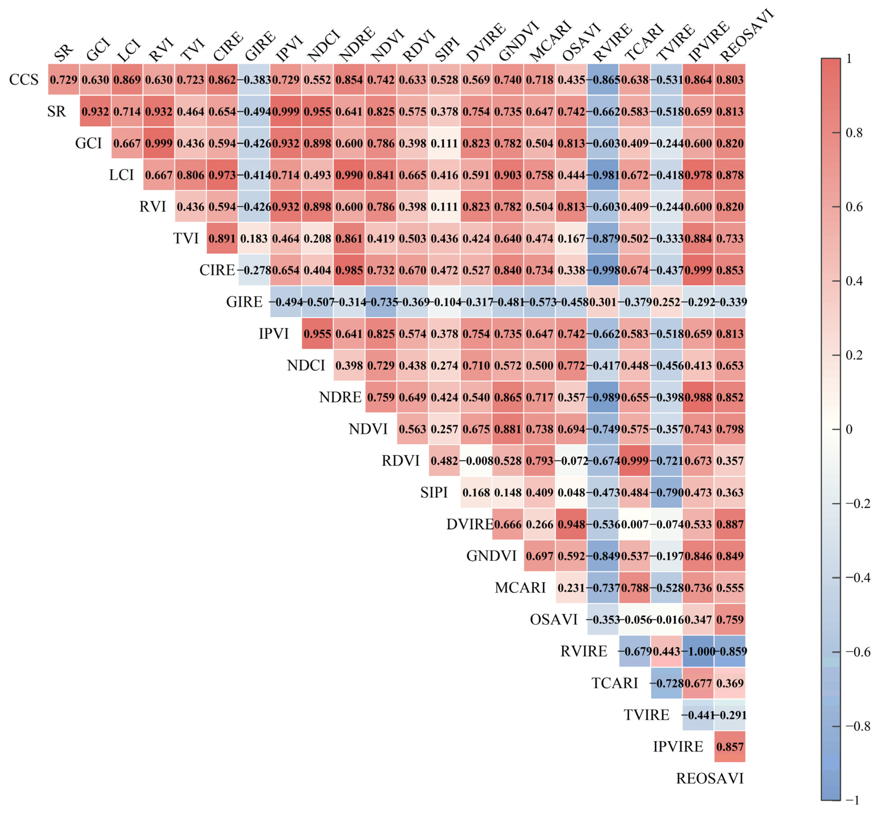
3.1. Correlation Analysis

The Pearson correlation analysis was conducted on the single-band spectral reflectance collected by the UAV and the CCS, with the results presented in Table 2. As shown in the table, except for the G band, all other single bands exhibit a significant correlation with the CCS (p < 0.01). Specifically, the R and B bands show a negative correlation with the CCS, while the NIR and RE bands display a positive correlation. Among these, the RE band demonstrates the highest correlation with the CCS, with a correlation coefficient of 0.682, followed by the NIR band with a correlation coefficient of 0.638. Within the visible light spectrum, the R band exhibits the highest correlation with the CCS, with a correlation coefficient of −0.446.
A Pearson correlation analysis was performed on the selected 21 vegetation indices and the CCS (Figure 4). The results indicate that except for GIRE, RVIRE, and TVIRE, the remaining 19 vegetation indices are positively correlated with CCS, with significant correlations observed between CCS and the selected vegetation indices. Among them, LCI exhibits the highest correlation with CCS, with a correlation coefficient of 0.869, followed by RVIRE, IPVIRE, and CIre, with correlation coefficients of −0.865, 0.864, and 0.862, respectively. In contrast, GIRE shows the lowest correlation with CCS, with a correlation coefficient of −0.383.

3.2. Principal Component Analysis

From the correlation analysis between vegetation indices and CCS, it can be seen that there is a significant correlation between the vegetation indices constructed in this study and the measured CCS, and at the same time, there is a strong correlation between these vegetation indices; therefore, this study utilized the SPSS 25 software to carry out the principal component analysis on the 21 vegetation indices constructed, and to reduce the dimensionality of the data in order to eliminate the multicollinearity between the factors, while retaining the information of the original data. The principal components extracted after principal component analysis, and the scores of each factor are shown in Table 3.
The principal component analysis extracted four main components in each vegetation index, and the cumulative contribution rate of the four components reached 94%, which contained the vast majority of the information of the original parameters, and could replace the original parameters to build the prediction model.

3.3. Modeling Results

In this paper, PLSR was selected to build a CCS inversion model with 21 vegetation indices as independent variables and measured CCS as dependent variable, and four principal components were selected based on the cumulative contribution of the independent variables, and the results showed (Figure 5a) that the RPDs of the model’s training and test dataset were 2.306 and 2.185, respectively, which were greater than 2, and that the model possessed a better predictive ability of the samples; the RMSEs for both were 2.230 and 2.922, the R2s were 0.807 and 0.770, and the slopes of the fitted regression lines were 0.772 and 0.868, respectively. Compared with the training dataset, the slope of the regression line in the test dataset is closer to 1:1, but the overall prediction value of the test dataset is low and more discrete. Overall, the PLSR model has good predictive ability and can be used for CCS prediction.
In the inversion model built based on the RF algorithm, the parameters were selected using the grid search method, and the number of decision trees was finally selected to be 170, the maximum depth of the decision tree was 5, the minimum number of samples required to split the internal nodes was 5, the minimum number of samples required on the leaf nodes was 1, and the maximum number of features considered in the node splitting was 23. The training results show (Figure 5b) that the model’s RPD for the training dataset and test dataset are 2.104 and 1.935, respectively, both higher than 1.4, and the model is able to predict the samples efficiently; the RMSEs for both are 2.471 and 2.937, respectively, and the R2s are 0.763 and 0.771, respectively, and the ratio of predicted and actual values of the model’s test dataset is much closer to 1:1 in the interval of CCS < 50, and the ratio of predicted and actual values of the model’s test dataset is much closer to 1:1 in the interval of SPAD > 50; the predicted CCS of the model is slightly lower than the measured CCS. Overall, the predictive ability of the CCS inversion model built based on the RF algorithm is good and can be used for CCS prediction.
The BPNN model is mainly composed of input, hidden and output layers, and its hyperparameters mainly include the number of hidden layers and neurons, the learning rate, the number of training times, and the activation function. Among them, the number of layers of the neural network and the number of neurons in the hidden layer can affect the performance of the model to a large extent. Theoretically, the deeper the number of hidden layers, the stronger the model’s ability to fit the function, but deeper layers may also bring problems such as overfitting; therefore, according to the trial-and-error method, this study chose to construct a neural network model containing four hidden layers.
When the number of nodes in the neural network is too large, not all neurons in the hidden layer can be adequately trained due to the limited amount of information in the training dataset, thus leading to overfitting. Even if the amount of information in the training data is sufficient, too many neurons in the hidden layer will increase the training time, thus making it difficult to achieve the expected results. Therefore, choosing the appropriate number of hidden layer neurons is equally important. The learning rate, as another important hyperparameter in the neural network model, controls how the gradient moves in each iteration to reach the optimal solution of the loss function, and its size determines the speed of the neural network’s learning speed, and the appropriate learning rate can make the cost function converge to the minimum value at a suitable speed. The number of training times also has an important impact on the model performance, as too many training times will lead to overfitting of the model, while too few will easily lead to underfitting. Therefore, based on the previous research, this study adopts the “trial and error method”, and finally sets the number of hidden layer neurons to 10, the learning rate to 0.001, and the number of training times to 200,000.
In addition, the activation function is the core parameter for neural networks to learn, understand and learn complex nonlinear functions; in this study, the construction of each hidden layer of the neural network used the hyperbolic tangent function (Tanh), which outputs between −1 and 1, and it solves the problem that the Sigmoid function does not output centred on 0.
In addition to this, regularization is used in this study to limit the range of values of the model parameters as a way to prevent overfitting of the BPNN model. The regularization method is divided into L1 regularization and L2 regularization, in which L1 regularization makes the model more inclined to select sparse features by adding a penalty term of L1 paradigm to the loss function of the model, which reduces unnecessary feature weights and improves the generalization ability, and L2 regularization quadratically constrains the parameters by summing up the squares of the individual elements in the weight vector and then solving for the square root to make the optimization solution stable fast, and makes the weights smoother. Compared with L1 regularization, L2 regularization is more robust to outliers. In the construction of the BPNN-based chest diameter inversion model, L2 regularization is adopted for the constraints of the loss function, and its parameter is set to 0.0001.
Meanwhile, based on the results of principal component analysis of vegetation indices, this study constructed a CCS inversion model of the BPNN algorithm with the four component factors obtained from the weighted calculation of 21 vegetation indices as the independent variables, and the training results showed (Figure 5c) that the RPDs of the model’s training and test dataset were 2.157 and 1.942, respectively, which were higher than 1.4, and that the model was able to predict the samples effectively; the two RMSEs are 2.138 and 2.607, and the R2s are 0.816 and 0.812, respectively, and the fitted regression lines of the training and test dataset are closer to the 1:1 regression line, with no systematic overestimation or underestimation, and in general, the prediction ability of the CCS inversion model based on the BPNN is better, and it is able to be used for the prediction of CCS.
In conclusion, the selected inversion algorithms in this study demonstrate good predictive abilities. However, based on a comprehensive assessment using R2 and RMSE, the BPNN model had the best predictive performance, highest accuracy, and least dispersion on the test dataset, making it the best choice for CCS inversion.

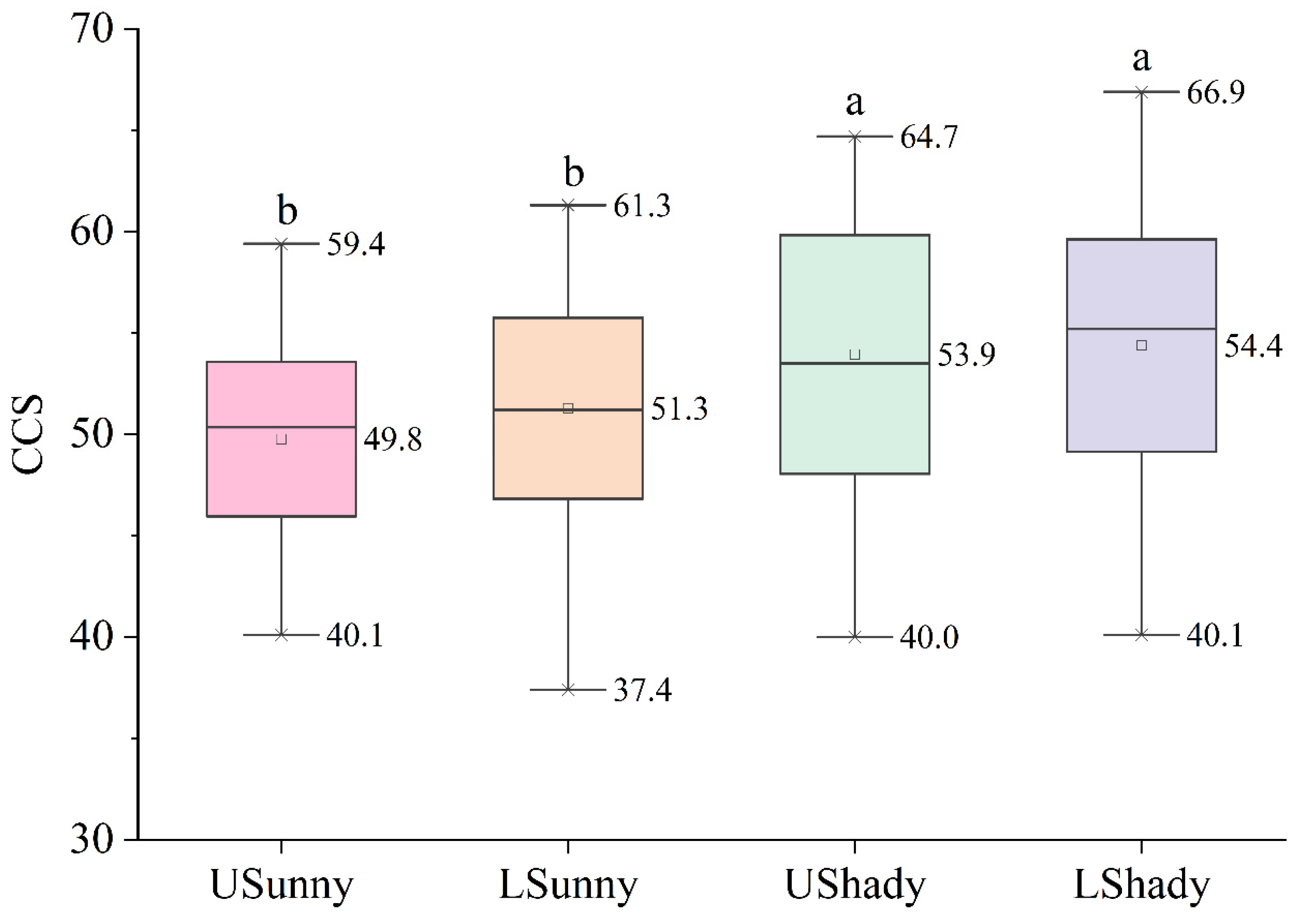
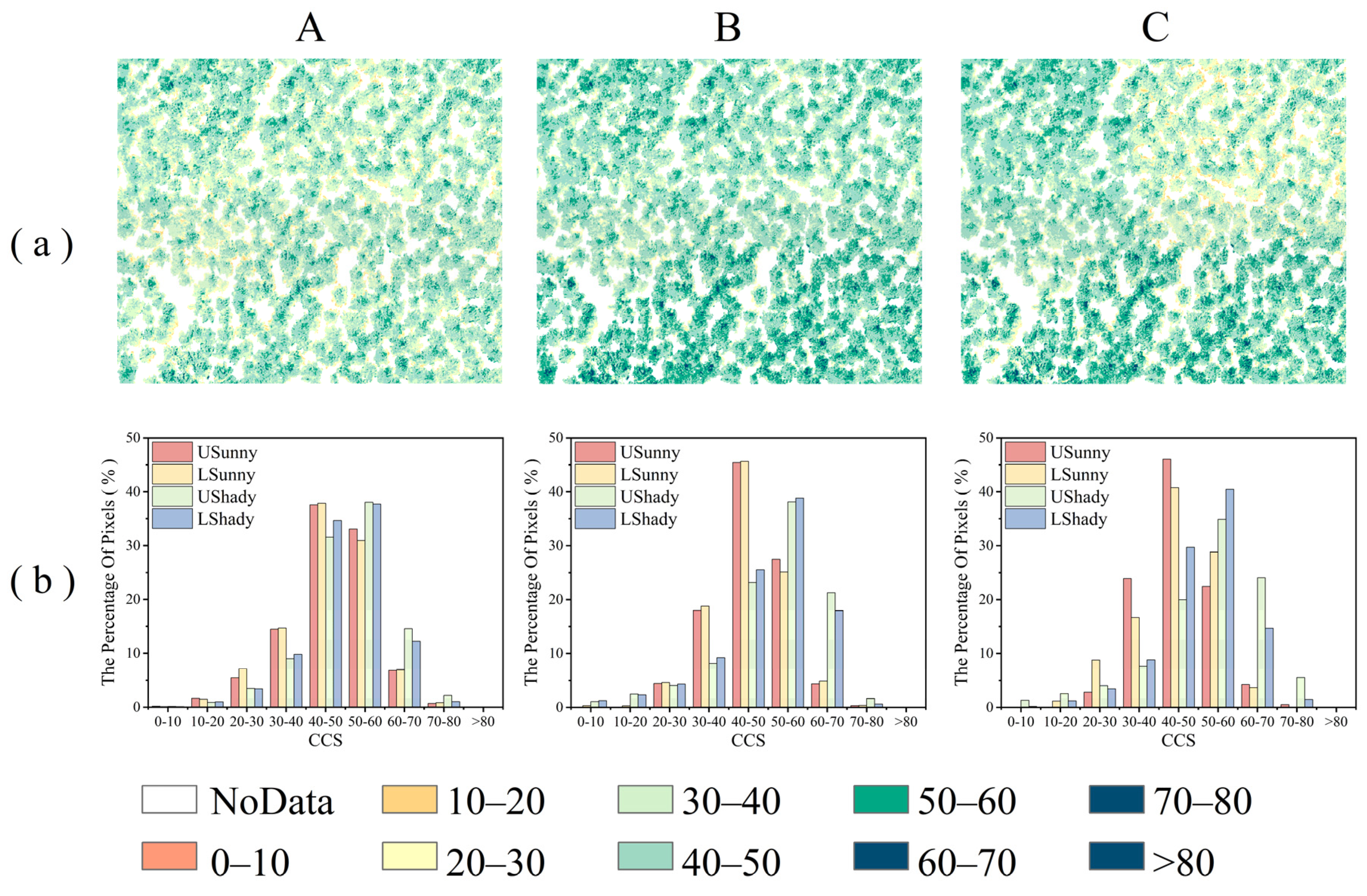
3.4. Effects of Terrain on CCS Estimates

Based on the selected optimal CCS inversion model, the CCS of USunny, LSunny, UShady and LShady were inverted and the results are shown in Figure 6. It is obvious that the pre-predicted CCSs of UShady and LShady are close to the 1:1 regression line, with R2s of 0.791 and 0.803, respectively, and RPDs of 1.636 and 1.779, respectively, which are higher than 1.4, indicating that the models have good predictive ability for these sites. On the other hand, the predicted TCCs for USunny and LSunny were slightly lower than the actual TCCs, with R2s of 0.662 and 0.659 and RPDs of 1.638 and 1.076, respectively, where the RPD for LSunny was below 1.4, indicating the effective prediction ability of the model for these locations.
When comparing the predicted CCS results for the four different terrains, it is evident that the model’s prediction accuracy is relatively similar for the upper and lower locations within the same slope location, with no significant differences in prediction capabilities. However, the selected best CCS model has significantly higher prediction accuracy and capability for samples on the shady slope compared to the sunny slope within the same slope direction. This indicates that slope direction can influence the accuracy of model predictions. Therefore, the best CCS model used in this study may not be applicable for predicting CCS of different slope directions.
Using the above conclusions, the training dataset was divided into two subsets: the sunny slope dataset and the shady slope dataset. The BPNN algorithm was then utilized to construct two separate CCS models: the sunny CCS model and the shady CCS model. Figure 7 illustrates the model prediction results and their performance on different slope locations. Both the sunny CCS model and shady CCS model achieved R2s of around 0.8, with RPDs of 2.381 and 2.015, respectively, both exceeding 2, indicating that both models have good sample predictive capabilities. The CCS of USunny and LSunny was predicted using the sunny CCS model, and the prediction results had an R2 above 0.8 in both cases. Similarly, applying the shady CCS model to predict the CCS on the UShady and LShady resulted in an R2 around 0.8 as well. This demonstrates that both models are highly adaptable to different slope direction and can be used to predict CCS in various terrains.
The training dataset was divided into USunny dataset, LSunny dataset, UShady dataset, and LShady dataset. Based on the BPNN algorithm, separate models were built for USunny CCS model, LSunny CCS model, UShady CCS model, and LShady CCS model. Table 4 shows the accuracy assessment of modeling and testing for the four models. With the exception of UShuuy, all models achieved an accuracy of above 0.8, with RPD > 2, indicating that they all possess good predictive capabilities and accurate CCS forecasting.
The study predicted the CCS in the study area using three categories of CCS inversion models, where the first category is the best CCS inversion model, while the second category includes the sunny CCS model and the shady CCS model. The third category comprises the USunny CCS model, LSunny CCS model, UShady CCS model, and LShady CCS model. Figure 8a shows the spatial distribution of predicted CCS for the three categories of CCS inversion models. The predictions of the first type of model differed significantly from the other two, with higher predictions in the sunny slope directions and lower predictions in the shady slope directions, whereas the second category model’s CCS distribution is more similar to that of the third category model. Figure 8b illustrates the pixel distribution among CCS for the three categories of CCS inversion models. The proportion of pixels with CCS between 50–60 is the highest in all three predicted maps, whereas the proportion of pixels with CCS greater than 80 is the lowest. The predicted CCS for the shady slope is noticeably higher than that for the sunny slope across different terrains. However, there is no significant difference in the predicted CCS between the upper and lower slope locations. The distribution of CCS predictions in the 40–60 interval is similar between the first and third category models, but there is a notable overestimation in intervals higher than 60, indicating some error in CCS prediction by the first category model. However, the spatial distribution of CCS predicted by the third category and the second category models is similar, which confirms the applicability of the second category models across various terrains.

4. Discussion

An analysis of the correlation between the selected 21 vegetation indices and CCS revealed that LCI, IPVIRE, and RVIRE displayed the highest correlation and explanatory power concerning CCS. This finding contrasts with the conclusion of Yuan et al. regarding the higher expressive capability of MCARI for predicting SPAD based on multispectral images of Hopea hainanensis [59]. It is known from previous studies on the correlation between SPAD and vegetation indices that the interpretation of SPAD varies among different plant species [60,61,62,63]. The spectral characteristics of plants are influenced by their unique structures, morphologies, and physiological features, and the biochemical composition and structure differ among different plant species, leading to varying absorption and reflection capacities of leaves in each spectral band. This divergence results in different plant populations’ spectral characteristics having varying capabilities in interpreting SPAD.
Moreover, the involvement of the red-edge band in constructing these three vegetation indices demonstrates the red-edge band’s heightened sensitivity to changes in SPAD. In this study’s correlation analysis between the five spectral images collected by drones and CCS, a highly significant correlation at the 0.01 level was observed between the red-edge band and CCS. This conclusion, similar to the findings of Lu et al. in predicting SPAD of Cinnamomum camphora dwarf forest using drone multispectral images [64], further confirms the interpretive capability of the red-edge band for SPAD.
In addition to the choice of vegetation indices, the choice of modeling methods is another important factor affecting the estimation of CCS. Previous studies have shown that machine learning algorithms have stronger generalization capabilities and better predictive performance in constructing SPAD models compared to traditional linear models due to their robust noise resistance [65,66,67].
In this study, based on a comprehensive analysis of R2, RPD, and RMSE, the performance of a traditional linear model (PLSR) was compared with three machine learning models (SVR, RMSE, and BPNN). The results showed that the BPNN model, which uses backpropagation to iteratively adjust model weights, had the best predictive ability in CCS estimation. This conclusion is consistent with previous research indicating that the BPNN model performs better in constructing SPAD inversion models [60,68]. Compared with other machine learning algorithms, BPNN takes the backpropagation algorithm as the core, and adjusts the BPNN model weights and biases by continuously repeating the forward and backward propagation process of data and errors, so as to fit the complex mapping relationship between the input and output data from a large number of training data, and iteratively obtains higher network performance.
However, compared to the significant advantage of the BPNN model in SPAD inversion, PLSR is significantly better at predicting CCS than RF. This suggests that the linearity or nonlinearity of the model did not have a large impact on the construction of the CCS model, which is inconsistent with the conclusions reached in most studies, but is more similar to the findings of Jiang et al. in the estimation of chlorophyll in watersheds [69]. This may be due to the fact that the CCS measured in this study was centrally distributed around 50, making the RF overly concerned with data in that range, leading to a decrease in overall prediction accuracy. In addition, the strong correlation among the selected vegetation indices as shown in Figure 4 suggests potential multicollinearity among the features, and the PLSR model developed from principal component analysis effectively addresses issues of high intercorrelation among variables, resulting in comparable predictive accuracy among the three models. Therefore, future optimization efforts could focus on refining the choice of vegetation indices or considering multiple types of independent variables to reduce multicollinearity between variables.
Although the best CCS model established in this study has good prediction ability, the prediction accuracy of the model appears to be significantly different among different terrains, and unlike the model’s stable prediction ability among different slope locations, its prediction generalization is lower among different slope directions. Compared with slope location, slope directions have a greater impact on the prediction accuracy of the best CCS model, making the model not applicable to CCS prediction in different terrains.
The interpretation of multispectral imagery for CCS is mainly derived from the reflectance of the Cunninghamia lanceolata canopy to solar radiation, which is directly related to the radiation environment of the vegetation canopy. Variations in the radiation environment of the vegetation canopy are mainly defined by the quantity, quality, and directional distribution of incident radiation, and these factors are mainly defined by the dimension and terrain of the vegetation site.
The interpretation of CCS from multispectral imagery is mainly derived from the reflectance of the Cunninghamia lanceolata canopy to solar radiation, which is directly related to the radiation environment of the vegetation canopy. Variations in the radiation environment of the vegetation canopy are defined by the quantity, quality, and directional distribution of incident radiation, and these factors are mainly defined by the latitude and terrain of the vegetation site.
The different performance of the best CCS model in slope location and slope directions may be due to the fact that the study area is located in a hilly area, and there is not much difference in elevation between different slope locations, so there is no big difference in the quality and quantity of solar radiation received by the Cunninghamia lanceolata canopy between different slope locations, while the slope directions have a big influence on the incidence direction of solar radiation, and a change in the slope directions will lead to the difference in the incidence angle of radiation, which will directly affect the reflectance of Cunninghamia lanceolata. The effect of the change of slope directions will lead to the difference of radiation incidence angle, which will directly affect the reflectance of the fir canopy, and the result of this effect is that the more the slope directions are turned to the light-facing direction, the larger the spectral reflectance ratio is [70]. Additionally, as a heliophilous species, Cunninghamia lanceolata experiences different light and water distribution across various slope aspects, directly influencing its growth, yield, and function [71,72]. These internal variations cannot be perfectly interpreted by vegetation indices, thus limiting the model’s adaptability. Based on the above factors, the following ways can be used in the future to reduce the influence of slope directions on the model prediction accuracy. First, the acquisition of multispectral images of the study area can be carried out at noon in cloudy weather as much as possible to reduce the influence of the directionality of solar radiation. Secondly, tilt photography can be used to obtain multi-angle multispectral information of the forest floor, and optimize the acquisition of spectral data of the forest floor from the perspective of forest canopy reflectance anisotropy [73], so as to reduce the influence of slope directions on spectral reflectance data. In addition, the feature parameters related to CCS can be further explored, and new vegetation indices or texture feature indices can be incorporated to achieve higher interpretation capability of CCS, so as to explore the CCS inversion model with better applicability.
However, as far as the above approaches are concerned, they do not completely eliminate the influence of terrain on the predictive ability of the model, so this study builds inverse models of CCS for different slope directions separately, aiming to seek for a better accuracy of CCS prediction. The model training results show that the sunny CCS model and the shady CCS model had higher predictive accuracy than the best CCS inversion model. Moreover, the predictive capabilities of the sunny CCS model and the shady CCS model did not vary significantly across different slope directions. Comparing the performance of the second category models and the third category models in predicting CCS across the study area, all six models exhibited strong predictive abilities with high similarity in the distribution patterns of CCS predictions. This confirms that the sunny CCS model and the shady CCS model have strong applicability across terrains. Therefore, in practical applications, separating inversion models for shady and sunny slopes can provide more accurate predictions of CCS. In addition, this study did not address the effect of elevation on model applicability.
In addition, there is still room for improvement in the following processes in this study: first, in the previous study, the SPAD can be calibrated to chlorophyll content with high accuracy, but there are still some errors in it [74,75], so this study can be followed up with a study on how to calibrate the CCS derived from the prediction to Cunninghamia lanceolata canopy chlorophyll content; second, this study has not elaborated on the effect of elevation on the applicability of the model, and so the model could not be applied in the prediction of CCS with large differences in stand elevation; third, this study used UAV remote sensing to estimate CCS with the aim of reducing the drawbacks of small range and long time in the investigation of chlorophyll process, but this study found that UAVs still have some limit in the investigation range in practical application due to signal reception and other problems, and currently, high-resolution satellites covering the whole world are constantly emerging, and scholars are also exploring the joint use of UAV and satellite data to carry out remote sensing investigations [76,77,78], so this study can be followed up with joint high-resolution satellite remote sensing to expand the application range of the CCS inversion model.

5. Conclusions

This study constructed a CCS inversion model based on multispectral images of near-mature Cunninghamia lanceolata forests acquired by drones and data from 200 collected SPAD samples. The research analyzed the terrain adaptability of the model, and the results showed the following:
Based on the correlation analysis between measured CCS and features extracted from multispectral drone images, a highly significant correlation at the 0.01 level was found between the red-edge band and CCS. The three vegetation indices with the highest correlation to CCS were LCI, RVIRE, and IPVIRE, all of which included the red-edge band in their construction, further confirming the close relationship between the red-edge band and CCS.
The principal component analysis of the vegetation indices constructed in this study shows that the correlation between the 21 vegetation indices is significant, and after dimensionality reduction of the vegetation index data, we can obtain four uncorrelated principal components, whose cumulative contribution rate is 94%, which contains most of the information of the original parameters, and can be used to establish prediction models instead of the original parameters.
Through a comprehensive analysis of R2, RPD, and RMSE, the BPNN model was identified as the best CCS model for predicting CCS. The model showed good performance with R2s of 0.816 and 0.812 for the training and test datasets, RMSEs of 2.138 and 2.607, and RPDs of 2.157 and 1.942, indicating high prediction accuracy and suitability for CCS prediction.
Using the established best CCS model, CCS was predicted for different terrains. The results showed similar prediction accuracy for CCS across different slope locations, but lower generalization across different slope directions. After separately modeling samples from different slope directions, both models showed R2 above 0.8 and demonstrated strong applicability across terrains.

Author Contributions

Conceptualization, R.L.; Investigation, L.Z., Y.Z., W.G. and N.C.; Methodology, L.Z., X.S. and R.L.; Software, L.Z. and H.L.; Validation, X.S.; writing—original draft preparation, L.Z.; writing—review and editing, H.L. All authors have read and agreed to the published version of the manuscript.

Funding

This work was supported by the Forestry Peak Discipline Construction Project of Fujian Agriculture and Forestry University (72202200205).

Data Availability Statement

The data is available on request from the corresponding author.

Conflicts of Interest

The authors declare no conflict of interest.

References

  1. Zhang, R.; Yang, P.; Liu, S.; Wang, C.; Liu, J. Evaluation of the Methods for Estimating Leaf Chlorophyll Content with SPAD Chlorophyll Meters. Remote Sens. 2022, 14, 5144. [Google Scholar] [CrossRef]
  2. Li, J.; Lu, X.; Ju, W.; Li, J.; Zhu, S.; Zhou, Y. Seasonal changes of leaf chlorophyll content as a proxy of photosynthetic capacity in winter wheat and paddy rice. Ecol. Indic. 2022, 140, 109018. [Google Scholar] [CrossRef]
  3. Phaenark, C.; Seechanhoi, P.; Sawangproh, W. Metal toxicity in Bryum coronatum Schwaegrichen: Impact on chlorophyll content, lamina cell structure, and metal accumulation. Int. J. Phytoremediation 2024, 26, 1336–1347. [Google Scholar] [CrossRef]
  4. Meng, F.; Chen, Z.; Wang, Y.; Multi-omics Analysis of Chlorophyll Metabolic Pathways in Tea Tree Varieties with Different Leaf Colors. Molecular Plant Breeding. 2024. Available online: https://link.cnki.net/urlid/46.1068.S.20240305.1556.008.html (accessed on 7 March 2024). (In Chinese).
  5. Fu, X.Y.; Mo, W.P.; Zhang, J.Y.; Zhou, L.Y.; Wang, H.C.; Huang, X.M. Shoot growth pattern and quantifying flush maturity with SPAD value in litchi (Litchi chinensis Sonn.). Sci. Hortic. 2014, 174, 29–35. [Google Scholar] [CrossRef]
  6. Rakib, M.; Borhan, A.; Jawahir, A. The relationship between SPAD chlorophyll and disease severity index in Ganoderma-infected oil palm seedlings. J. Bangladesh Agric. Univ. 2019, 17, 355–358. [Google Scholar] [CrossRef]
  7. Celaleddin, B.; Irem, T.; Hatice, T.; Mehmet, Y.; Mujde, K. Spad greenness to estimate genotypic variation in flag leaf chlorophyll in spring wheat under Mediterranean conditions. Turk. J. Field Crops 2015, 20, 1–8. [Google Scholar]
  8. Saberioon, M.M.; Amin, M.S.M.; Anuar, A.R.; Gholizadeh, A.; Wayayok, A.; Khairunniza-Bejo, S. Assessment of rice leaf chlorophyll content using visible bands at different growth stages at both the leaf and canopy scale. Int. J. Appl. Earth Obs. Geoinf. 2014, 32, 35–45. [Google Scholar] [CrossRef]
  9. Nguyen, H.T.; Lee, B.-W. Assessment of rice leaf growth and nitrogen status by hyperspectral canopy reflectance and partial least square regression. Eur. J. Agron. 2006, 24, 349–356. [Google Scholar] [CrossRef]
  10. Zarco-Tejada, P.; Hornero, A.; Beck, P.; Kattenborn, T.; Kempeneers, P.; Hernández-Clemente, R. Chlorophyll content estimation in an open-canopy conifer forest with Sentinel-2A and hyperspectral imagery in the context of forest decline. Remote. Sens. Environ. 2019, 223, 320–335. [Google Scholar] [CrossRef]
  11. Delloye, C.; Weiss, M.; Defourny, P. Retrieval of the canopy chlorophyll content from Sentinel-2 spectral bands to estimate nitrogen uptake in intensive winter wheat cropping systems. Remote. Sens. Environ. 2018, 216, 245–261. [Google Scholar] [CrossRef]
  12. Wan, L.; Ryu, Y.; Dechant, B.; Lee, J.; Zhong, Z.; Feng, H. Improving retrieval of leaf chlorophyll content from Sentinel-2 and Landsat-7/8 imagery by correcting for canopy structural effects. Remote Sens. Environ. 2024, 304, 114048. [Google Scholar] [CrossRef]
  13. Li, Y.; Ma, Q.; Chen, J.M.; Croft, H.; Luo, X.; Zheng, T.; Rogers, C.; Liu, J. Fine-scale leaf chlorophyll distribution across a deciduous forest through two-step model inversion from Sentinel-2 data. Remote. Sens. Environ. 2021, 264, 112618. [Google Scholar] [CrossRef]
  14. Vincini, M.; Calegari, F.; Casa, R. Sensitivity of leaf chlorophyll empirical estimators obtained at Sentinel-2 spectral resolution for different canopy structures. Precis. Agric. 2016, 17, 313–331. [Google Scholar] [CrossRef]
  15. Zhang, S.; Zhao, G.; Lang, K.; Su, B.; Chen, X.; Xi, X.; Zhang, H. Integrated Satellite, Unmanned Aerial Vehicle (UAV) and Ground Inversion of the SPAD of Winter Wheat in the Reviving Stage. Sensors 2019, 19, 1485. [Google Scholar] [CrossRef] [PubMed]
  16. Croft, H.; Chen, J.; Zhang, Y.; Simic, A. Modelling leaf chlorophyll content in broadleaf and needle leaf canopies from ground, CASI, Landsat TM 5 and MERIS reflectance data. Remote. Sens. Environ. 2013, 133, 128–140. [Google Scholar] [CrossRef]
  17. Colomina, I.; Molina, P. Unmanned aerial systems for photogrammetry and remote sensing: A review. ISPRS J. Photo-Grammetry Remote Sens. 2014, 92, 79–97. [Google Scholar] [CrossRef]
  18. Jihoon, S.; Gunhyeong, L.; TaeHo, K.; Hwa, C.K.; Min, H.S.; Hyuck, K.D.; JongCheol, P.; YoonKyung, C. Deep learning-based efficient drone-borne sensing of cyanobacterial blooms using a clique-based feature extraction approach. Sci. Total Environ. 2023, 912, 169540. [Google Scholar]
  19. Zhang, A.; Yin, S.; Wang, J.; He, N.; Chai, S.; Pang, H. Grassland Chlorophyll Content Estimation from Drone Hyperspectral Images Combined with Fractional-Order Derivative. Remote Sens. 2023, 15, 5623. [Google Scholar] [CrossRef]
  20. Sahoo, R.N.; Gakhar, S.; Rejith, R.G.; Verrelst, J.; Ranjan, R.; Kondraju, T.; Meena, M.C.; Mukherjee, J.; Daas, A.; Kumar, S.; et al. Optimizing the Retrieval of Wheat Crop Traits from UAV-Borne Hyperspectral Image with Radiative Transfer Modelling Using Gaussian Process Regression. Remote Sens. 2023, 15, 5496. [Google Scholar] [CrossRef]
  21. Chuanmei, Z.; Jianli, D.; Zipeng, Z.; Jinjie, W.; Zheng, W.; Xiangyue, C.; Jingzhe, W. SPAD monitoring of saline vegetation based on Gaussian mixture model and UAV hyperspectral image feature classification. Comput. Electron. Agric. 2022, 200, 107236. [Google Scholar]
  22. Lv, S.; Wang, J.; Wang, S.; Wang, Q.; Wang, Z.; Fang, Y.; Zhai, W.; Wang, F.; Qu, G.; Ma, W. Quantitative analysis of chlorophyll in Catalpa bungei leaves based on partial least squares regression and spectral reflectance index. Sci. Hortic. 2024, 329, 113019. [Google Scholar] [CrossRef]
  23. Xiao, H.; Beibei, N.; Xinju, L.; Xiangyu, M. Unmanned aerial vehicle (UAV) remote sensing estimation of wheat chlorophyll in subsidence area of coal mine with high phreatic level. Earth Sci. Inform. 2021, 14, 2171–2181. [Google Scholar]
  24. Naqvi, S.M.Z.A.; Awais, M.; Khan, F.S.; Afzal, U.; Naz, N.; Khan, M.I. Unmanned air vehicle based high resolution imagery for chlorophyll estimation using spectrally modified vegetation indices in vertical hierarchy of citrus grove. Remote Sens. Appl. Soc. Environ. 2021, 23, 100596. [Google Scholar]
  25. Wang, Y.; Tan, S.; Jia, X.; Qi, L.; Liu, S.; Lu, H.; Wang, C.; Liu, W.; Zhao, X.; He, L.; et al. Estimating relative chlorophyll content in rice leaves using unmanned aerial vehicle multi-spectral images and spectral-textural analysis. Agronomy 2023, 13, 1541. [Google Scholar] [CrossRef]
  26. Li, C.; Ma, C.; Chen, P.; Cui, Y.; Shi, J.; Wang, Y. Machine learning-based estimation of potato chlorophyll content at different growth stage using UAV hyperspectral data. Zemdirb. Agric. 2021, 108, 181–190. [Google Scholar] [CrossRef]
  27. Qian, S.; Xiaohe, G.; Liping, C.; Xiaobin, X.; Zhonghui, W.; Yuchun, P.; Yunbing, G. Monitoring maize canopy chlorophyll density under lodging stress based on UAV hyperspectral imagery. Comput. Electron. Agric. 2022, 193, 106671. [Google Scholar]
  28. Huaixing, X.; Juzhong, W.; Yiling, Q.; Lulu, H.; Yan, T.; Zhongsheng, Z.; Xiaojun, X.; Yufeng, Z. Estimating Leaf Chlorophyll Content of Moso Bamboo Based on Unmanned Aerial Vehicle Visible Images. Remote Sens. 2022, 14, 2864. [Google Scholar] [CrossRef]
  29. Songtao, B.; Weizhen, L.; Minglu, T.; Qi, W.; Tao, Y.; Qingrui, C.; Linyi, L. Rice Leaf Chlorophyll Content Estimation Using UAV-Based Spectral Images in Different Regions. Agronomy 2022, 12, 2832. [Google Scholar] [CrossRef]
  30. Wang, B.; Wang, Z.; Zhang, D.; Li, L.; Zhao, Y.; Luo, T.; Wang, X. Spatial and Temporal Variation in Primary Forest Growth in the Northern Daxing’an Mountains Based on Tree-Ring and NDVI Data. Forests 2024, 15, 317. [Google Scholar] [CrossRef]
  31. State Forestry and Grassland Administration. China Forest Resources Report (2014–2018); China Forestry Press: Beijing, China, 2019. (In Chinese) [Google Scholar]
  32. Lu, L.-H.; Nong, Y.; Li, H.; Zeng, J.; Sun, D.-J.; Chen, L.; Ming, A.-G.; Yang, Y.-J. Effects of retention density on growth, biomass, and economic benefit of Cunninghamia lanceolata plantation. Chin. J. Appl. Ecol. 2020, 31, 717–724. (In Chinese) [Google Scholar]
  33. Zhang, W.Q.; Fang, L.; Yang, J.; Zhang, W.D.; Yan, Y.; Yan, Q.L. Reconstruction of stand-replacement disturbance and stand age of Chinese fir plantation based on a Landsat time series in Huitong County, Hunan. Chin. J. Ecol. 2018, 37, 3467–3479. (In Chinese) [Google Scholar]
  34. Zhou, X.; Hu, R.L. Analysis of the current situation of forest resources in state-owned forest farms in Shunchang County, Fujian Province. Inn. Mong. For. Investig. Des. 2021, 44, 13–19. (In Chinese) [Google Scholar]
  35. Wen, M.L.; Chen, Y.; He, X.W.; Yang, L.; Zhou, Q. Distribution of collapsed gullies (Beng Gang) using GIS and verification of slope aspect selection. Sci. Soil Water Conserv. 2018, 16, 1–7. (In Chinese) [Google Scholar]
  36. Luo, X.B.; Xie, T.S.; Dong, S.X. Estimation of Citrus Canopy Chlorophyll Based on UAV Multispectral Images. Trans. Chin. Soc. Agric. Mach. 2023, 54, 198–205. (In Chinese) [Google Scholar]
  37. Zou, X.; Jin, J.; Mõttus, M. Potential of Satellite Spectral Resolution Vegetation Indices for Estimation of Canopy Chlorophyll Content of Field Crops: Mitigating Effects of Leaf Angle Distribution. Remote Sens. 2023, 15, 1234. [Google Scholar] [CrossRef]
  38. Verma, B.; Prasad, R.; Srivastava, P.K.; Yadav, S.A.; Singh, P.; Singh, R. Investigation of optimal vegetation indices for retrieval of leaf chlorophyll and leaf area index using enhanced learning algorithms. Comput. Electron. Agric. 2022, 192, 106581. [Google Scholar] [CrossRef]
  39. Gitelson, A.A.; Gritz, Y.; Merzlyak, M.N. Relationships between leaf chlorophyll content and spectral reflectance and algorithms for non-destructive chlorophyll assessment in higher plant leaves. J. Plant Physiol. 2003, 160, 271–282. [Google Scholar] [CrossRef]
  40. Datt, B. A New Reflectance Index for Remote Sensing of Chlorophyll Content in Higher Plants: Tests using Eucalyptus Leaves. J. Plant Physiol. 1999, 154, 30–36. [Google Scholar] [CrossRef]
  41. Schuerger, A.C.; Capelle, G.A.; Di Benedetto, J.A.; Mao, C.; Thai, C.N.; Evans, M.D.; Richards, J.T.; Blank, T.A.; Stryjewski, E.C. Comparison of two hyperspectral imaging and two laser-induced fluorescence instruments for the detection of zinc stress and chlorophyll concentration in bahia grass (Paspalum notatum Flugge.). Remote. Sens. Environ. 2003, 84, 572–588. [Google Scholar] [CrossRef]
  42. Chen, Z.; Jia, K.; Wei, X.; Liu, Y.; Zhan, Y.; Xia, M.; Yao, Y.; Zhang, X. Improving leaf area index estimation accuracy of wheat by involving leaf chlorophyll content information. Comput. Electron. Agric. 2022, 196, 106902. [Google Scholar] [CrossRef]
  43. Gitelson, A.A.; Viña, A.; Arkebauer, T.J.; Rundquist, D.C.; Keydan, G.; Leavitt, B. Remote estimation of leaf area index and green leaf biomass in maize canopies. Geophys. Res. Lett. 2003, 30, 1248. [Google Scholar] [CrossRef]
  44. Dube, T.; Mutanga, O.; Elhadi, A.; Ismail, R. Intra-and-Inter Species Biomass Prediction in a Plantation Forest: Testing the Utility of High Spatial Resolution Spaceborne Multispectral Rapid Eye Sensor and Advanced Machine Learning Algorithms. Sensors 2014, 14, 15348–15370. [Google Scholar] [CrossRef]
  45. Gupta, S.K.; Pandey, A.C. PROSAIL and empirical model to evaluate spatio-temporal heterogeneity of canopy chlorophyll content in subtropical forest. Model. Earth Syst. Environ. 2021, 8, 2151–2165. [Google Scholar] [CrossRef]
  46. Hong, S.; Minzan, L.; Yane, Z.; Yong, Z.; Haihua, W. Detection of Corn Chlorophyll Content Using Canopy Spectral Reflectance. Sens. Lett. 2010, 8, 134–139. [Google Scholar] [CrossRef]
  47. Gu, C.; Li, J.; Liu, Q.; Zhang, H.; Liu, L.; Mumtaz, F.; Dong, Y.; Zhao, J.; Wang, X.; Liu, C. Retrieving decametric-resolution leaf chlorophyll content from GF-6 WFV by assessing the applicability of red-edge vegetation indices. Comput. Electron. Agric. 2023, 215, 108455. [Google Scholar] [CrossRef]
  48. Hajek, P.; Mörsdorf, M.; Kovach, K.R.; Greinwald, K.; Rose, L.; Nock, C.A.; Scherer-Lorenzen, M. Quantifying the influence of tree species richness on community drought resistance using drone-derived NDVI and ground-based measures of Plant Area Index and leaf chlorophyll in a young tree diversity experiment. Eur. J. For. Res. 2024, 143, 141–155. [Google Scholar] [CrossRef]
  49. Patrick, A.; Pelham, S.; Culbreath, A.; Holbrook, C.C.; De Godoy, I.J.; Li, C. High throughput phenotyping of tomato spot wilt disease in peanuts using unmanned aerial systems and multispectral imaging. IEEE Instrum. Meas. Mag. 2017, 20, 4–12. [Google Scholar] [CrossRef]
  50. Qian, B.; Ye, H.; Huang, W.; Xie, Q.; Pan, Y.; Xing, N.; Ren, Y.; Guo, A.; Jiao, Q.; Lan, Y. A sentinel-2-based triangular vegetation index for chlorophyll content estimation. Agric. For. Meteorol. 2022, 322, 109000. [Google Scholar] [CrossRef]
  51. Cao, Y.; Zhou, H.; Zheng, W. Study on Methods of Reducing Hyperspectral Data and Retrieving Chlorophyll Content from Rice Leaf. J. Shenyang Agric. Univ. 2019, 50, 101–107. (In Chinese) [Google Scholar]
  52. De Sousa, C.; Souza, C.G.; Zanella, L.; De Carvalho, L. Analysis of Rapideye’s Red edge band for image segmentation and classification. In Proceedings of the GEOBIA 2012: 4th International Conference on Geographic Object-Based Image Analysis, Rio de Janeiro, Brazil, 7–9 May 2012; Brazilian National Institute for Space Research: Paraiba Valley, Brazil, 2012; Volume 79, pp. 7–9. [Google Scholar]
  53. Zhang, L.; Han, W.; Niu, Y.; Chávez, J.L.; Shao, G.; Zhang, H. Evaluating the sensitivity of water stressed maize chlorophyll and structure based on UAV derived vegetation indices. Comput. Electron. Agric. 2021, 185, 106174. [Google Scholar] [CrossRef]
  54. Yang, G.; Niu, L. Retrieval of Chlorophyll Content in Ear Leaves of Summer Maize Based on UAV Multispectral Data. Acta Agric. Jiangxi 2022, 34, 8–12. (In Chinese) [Google Scholar]
  55. Nakaji, T.; Oguma, H.; Nakamura, M.; Kachina, P.; Asanok, L.; Marod, D.; Aiba, M.; Kurokawa, H.; Kosugi, Y.; Kassim, A.R.; et al. Estimation of six leaf traits of East Asian forest tree species by leaf spectroscopy and partial least square regression. Remote Sens. Environ. 2019, 233, 111381. [Google Scholar] [CrossRef]
  56. Yi, L.; Kangkang, W.; Ke, C.; Jianqiang, H.; Yong, Z.; Guang, Y.; Ning, Y.; Ben, N.; Bin, W.; Lei, W.; et al. Forecasting Monthly Water Deficit Based on Multi-Variable Linear Regression and Random Forest Models. Water 2023, 15, 1075. [Google Scholar] [CrossRef]
  57. Amirruddin, A.D.; Muharam, F.M.; Ismail, M.H.; Ismail, M.F.; Tan, N.P.; Karam, D.S. Hyperspectral remote sensing for assessment of chlorophyll sufficiency levels in mature oil palm (Elaeis guineensis) based on frond numbers: Analysis of decision tree and random forest. Comput. Electron. Agric. 2020, 169, 105221. [Google Scholar] [CrossRef]
  58. Dong, J.; Qin, W.; Mo, J. Low-Cost Multi-Objective Optimization of Multiparameter Antenna Structures Based on the l1 Optimization BPNN Surrogate Model. Electronics 2019, 8, 839. [Google Scholar] [CrossRef]
  59. Yuan, Y.; Wang, X.; Shi, M. Prediction of relative chlorophyll content in Hopea hainanensis based on multispectral frequency domain features. J. Beijing For. Univ. 2023, 45, 42–52. (In Chinese) [Google Scholar]
  60. Gao, C.; Li, H.; Wang, J.; Zhang, X.; Huang, K.; Song, X.; Yang, W.; Feng, M.; Xiao, L.; Zhao, Y.; et al. Combined use of spectral resampling and machine learning algorithms to estimate soybean leaf chlorophyll. Comput. Electron. Agric. 2024, 218, 108675. [Google Scholar] [CrossRef]
  61. Qifu, L.; Cong, X.; Xueyu, T.; Lihua, C.; Jingmin, J.; Yanjie, L. Estimating canopy chlorophyll in slash pine using multitemporal vegetation indices from uncrewed aerial vehicles (UAVs). Precis. Agric. 2024, 25, 1086–1105. [Google Scholar]
  62. Gao, G.; Zhang, L.; Wu, L.; Yuan, D. Estimation of Chlorophyll Content in Wheat Based on Optimal Spectral Index. Appl. Sci. 2024, 14, 703. [Google Scholar] [CrossRef]
  63. Tripathi, R.; Mohanty, S.; Swain, C.K.; Das, S.; Nayak, P.; Moharana, K.C.; Mohapatra, S.D.; Goud, B.R.; Raghu, S.; Sahoo, R.N.; et al. Predicting chlorophyll and nitrogen content in rice using multiple regression models. J. Plant Nutr. 2024, 47, 881–904. [Google Scholar] [CrossRef]
  64. Lu, X.; Wang, Q.; Zhang, H. Inversion of SPAD of Cinnamomum camphora Dwarf Forest Based on UAV Multispectral Remote Sensing. Trans. Chin. Soc. Agric. Mach. 2023, 54, 201–209. (In Chinese) [Google Scholar]
  65. Harpinder, S.; Ajay, R.; Raj, S.; Brijendra, P. Estimation of chlorophyll, macronutrients and water content in maize from hyperspectral data using machine learning and explainable artificial intelligence techniques. Remote Sens. Lett. 2022, 13, 969–979. [Google Scholar]
  66. Zhou, L.; Nie, C.; Su, T.; Xu, X.; Song, Y.; Yin, D.; Liu, S.; Liu, Y.; Bai, Y.; Jia, X.; et al. Evaluating the Canopy Chlorophyll Density of Maize at the Whole Growth Stage Based on Multi-Scale UAV Image Feature Fusion and Machine Learning Methods. Agriculture 2023, 13, 895. [Google Scholar] [CrossRef]
  67. Feng, H.; Yang, Z.; Chen, H. Estimation of Summer Maize SPAD Based on UAV Multispectral Images. Trans. Chin. Soc. Agric. Mach. 2022, 53, 211–219. (In Chinese) [Google Scholar]
  68. Zhang, X.; Yu, Z.; Li, H. Remote sensing estimation model of SPAD for rice leaves in Northeast China. J. China Agric. Univ. 2020, 25, 66–75. (In Chinese) [Google Scholar]
  69. Bo, J.; Hailong, L.; Qianguo, X.; Jiannan, C.; Xiangyang, Z.; Lin, L.; Sisi, L.; Zhiming, Z.; Huiyan, X.; Ling, M. Evaluating Traditional Empirical Models and BPNN Models in Monitoring the Concentrations of Chlorophyll-A and Total Suspended Particulate of Eutrophic and Turbid Waters. Water 2021, 13, 650. [Google Scholar] [CrossRef]
  70. Sun, W.-Q.; Zhao, Y.-S.; Tu, L.-L. Analysis of related factors of slope plant hyperspectral remote sensing. Spectrosc. Spectr. Anal. 2014, 34, 2495–2499. (In Chinese) [Google Scholar]
  71. Dong, C.; Fang, L. Association Analysis between the Site Index Model and the Site Factors of Cunninghamia lanceolata Timber Forest in Western Zhejiang Province. Nat. Environ. Polution Technol. 2019, 18, 359–368. [Google Scholar]
  72. Wu, N.; Li, Z.; Liao, S. Spectral Characteristics and Influencing Factors of Pinus kesiya var.langbianensis Based on Airborne Hyperspectral Technique. For. Res. 2018, 31, 63–68. (In Chinese) [Google Scholar]
  73. Deng, L.; Chen, Y.; Zhao, Y.; Zhu, L.; Gong, H.-L.; Guo, L.-J.; Zou, H.-Y. An approach for reflectance anisotropy retrieval from UAV-based oblique photogrammetry hyperspectral imagery. Int. J. Appl. Earth Obs. Geoinf. 2021, 102, 102442. [Google Scholar] [CrossRef]
  74. Coste, S.; Baraloto, C.; Leroy, C.; Marcon, É.; Renaud, A.; Richardson, A.D.; Roggy, J.-C.; Schimann, H.; Uddling, J.; Hérault, B. Assessing foliar chlorophyll contents with the SPAD-502 chlorophyll meter: A calibration test with thirteen tree species of tropical rainforest in French Guiana. Ann. For. Sci. 2010, 67, 607. [Google Scholar] [CrossRef]
  75. Donnelly, A.; Yu, R.; Rehberg, C.; Meyer, G.; Young, E.B. Leaf chlorophyll estimates of temperate deciduous shrubs during autumn senescence using a SPAD-502 meter and calibration with extracted chlorophyll. Ann. For. Sci. 2020, 77, 30. [Google Scholar] [CrossRef]
  76. Srivastava, P.K.; Rawat, R. Retrieval of leaf chlorophyll content using drone imagery and fusion with Sentinel-2 data. Smart Agric. Technol. 2023, 6, 100353. [Google Scholar] [CrossRef]
  77. El-Alem, A.; Chokmani, K.; Venkatesan, A.; Rachid, L.; Agili, H.; Dedieu, J.P. How Accurate Is an Unmanned Aerial Vehicle Data-Based Model Applied on Satellite Imagery for Chlorophyll-a Estimation in Freshwater Bodies? Remote Sens. 2021, 13, 1134. [Google Scholar] [CrossRef]
  78. Zhen, J.; Jiang, X.; Xu, Y.; Miao, J.; Zhao, D.; Wang, J.; Wang, J.; Wu, G. Mapping leaf chlorophyll content of mangrove forests with Sentinel-2 images of four periods. Int. J. Appl. Earth Obs. Geoinf. 2021, 102, 102387. [Google Scholar] [CrossRef]
Figure 1. Dichotomous slope direction division.
Forests 15 00965 g001
Figure 2. Study area and sample distribution.
Forests 15 00965 g002
Figure 3. Measured CCS in different terrains. Values are maximum, mean, and minimum, respectively. According to one-way ANOVA, different letters above the box plots indicate significant differences in CCS among different terrains (p < 0.05).
Forests 15 00965 g003
Figure 4. Correlation analysis between vegetation index and CCS.
Forests 15 00965 g004
Figure 5. Prediction results of CCS models established using PLSR (a), RF (b) and BPNN (c) algorithms. In this figure, the blue open circles are the results of the testing of the model training capability during the model training process, and the red open circles are the results of the prediction of the test set using the trained model. The red line is the 1:1 regression line.
Forests 15 00965 g005
Figure 6. CCS predictions of the best CCS model for USunny (a), LSunny (b), UShady (c), and LShady (d). The red line is the 1:1 regression line.
Forests 15 00965 g006
Figure 7. Predictive results and terrain applicability analysis of the Sunny CCS model (a) and the Shady CCS model (b). The black line is the 1:1 regression line.
Forests 15 00965 g007
Figure 8. Distribution of CCS predictions for the first category model (A), the second category model (B), and the third category model (C) in the study area (a) and the percentage of pixels between each CCS tier (b).
Forests 15 00965 g008
Table 1. Vegetation indices used in this study. B, G, R, RE, and NIR are the reflectance of the blue band, green band red band, red-edge band, and NIR band, respectively.
Vegetation IndexAcronymEquationReferences
Simple RatioSR N I R / G [38]
Green Chlorophyll IndexGCI N I R / G 1 [39]
Leaf Chlorophyll IndexLCI ( R E R ) / ( R E + G ) [40]
Ratio Vegetation IndexRVI N I R / G [41]
Triangular Vegetation IndexTVI 0.5 [ 120 N I R G 200 R G ] [42]
Red Edge Chlorophyll IndexCIre N I R / R E 1 [43]
Red-Edge Greenness IndexGIRE G / R E [44]
Infrared Percent Vegetation IndexIPVI N I R / ( N I R + R ) [45]
Normalized Difference Chlorophyll IndexNDCI ( R E R ) / ( R E + R ) [46]
Red-Edge Normalized Difference Vegetation IndexNDRE ( N I R R E ) / ( N I R + R E ) [47]
Normalized Difference Vegetation IndexNDVI ( N I R R ) / ( N I R + R ) [48]
Renormalized Difference Vegetation IndexRDVI ( N I R R ) / ( N I R + R ) [48]
Red-Edge Difference Vegetation IndexDVIRE N I R R E [49]
Green Normalized Difference Vegetation IndexGNDVI ( N I R G ) / ( N I R + G ) [50]
Modified Chlorophyll Uptake Ratio IndexMCARI R E R 0.2 R E G × R E / R [51]
Optimized Soil-Adjusted Vegetation IndexOSAVI 1.16 ( N I R R ) / ( N I R + R + 0.16 ) [37]
Red-Edge Ratio Vegetation IndexRVIRE R E / N I R [52]
Transformed Chlorophyll Absorption Reflectance IndexTCARI 3 [ N I R R 0.2 ( N I R G ) ( N I R / R ) [53]
Red-Edge Triangular Vegetation IndexTVIRE 0.5 [ 120 N I R G 200 R E G ] [44]
Red-Edge Infrared Percent Vegetation IndexIPVIRE N I R / ( N I R + R E ) [44]
Red-Edge Optimized Soil-Adjusted Vegetation IndexREOSAVI 1.16 ( N I R R E ) / ( N I R + R E + 0.16 ) [54]
Table 2. Correlation analysis between single-band spectral values and CCS. ** indicates that they are highly significantly correlated at the 0.01 level.
BandSPAD
R−0.446 **
G−0.097
B−0.216 **
NIR0.638 **
RE0.682 **
Table 3. Classification of principal components of vegetation index and scores of each factor.
Vegetation IndexPrincipal Component
1234
SR0.2440.141−0.1730.144
GCI0.2270.242−0.0430.038
LCI0.252−0.1060.153−0.114
RVI0.2270.242−0.0430.038
TVI0.188−0.2040.3660.211
CIRE0.241−0.1660.205−0.030
GIRE−0.133−0.1110.3390.469
IPVI0.2440.141−0.1730.144
NDCI0.2020.235−0.2920.172
NDRE0.241−0.1480.214−0.085
NDVI0.2420.090−0.083−0.250
RDVI0.183−0.305−0.259−0.100
SIPI0.120−0.247−0.1460.515
DVIRE0.1910.3220.1690.186
GNDVI0.2410.0440.142−0.265
MCARI0.209−0.166−0.167−0.255
OSAVI0.1660.4050.0270.085
RVIRE−0.2440.160−0.1950.039
TCARI0.185−0.299−0.261−0.098
TVIRE−0.1370.2470.360−0.376
IPVIRE0.243−0.1630.198−0.035
REOSAVI0.2460.1060.2060.108
Characteristic value13.8663.4482.0931.277
Accumulative contribution (%)63.02578.69788.20994.013
Table 4. Construction results of CCS inversion models for four different terrains based on BPNN algorithm.
Model TypeTraining DatasetTest Dataset
RMSERPDR2RMSERPDR2
USunny CCS model1.9042.2500.8452.0472.0590.793
LSunny CCS model1.3772.5140.8212.0562.4510.818
UShady CCS model2.1742.4640.8532.0292.5850.835
LShady CCS model1.5752.4650.8162.7192.0490.804
Disclaimer/Publisher’s Note: The statements, opinions and data contained in all publications are solely those of the individual author(s) and contributor(s) and not of MDPI and/or the editor(s). MDPI and/or the editor(s) disclaim responsibility for any injury to people or property resulting from any ideas, methods, instructions or products referred to in the content.

