Abstract
As a feature of global warming, climate change has been a severe issue in the 21st century. A more comprehensive reconstruction is necessary in the climate assessment process, considering the heterogeneity of climate change scenarios across various meteorological elements and seasons. To better comprehend the change in minimum temperature in winter in the Jinsha River Basin (China), we built a standard tree-ring chronology from Picea likiangensis var. balfouri and reconstructed the regional mean minimum temperature of the winter half-years from 1606 to 2016. This reconstruction provides a comprehensive overview of the changes in winter temperature over multiple centuries. During the last 411 years, the regional climate has undergone seven warm periods and six cold periods. The reconstructed temperature sensitively captures the climate warming that emerged at the end of the 20th century. Surprisingly, during 1650–1750, the lowest winter temperature within the research area was about 0.44 °C higher than that in the 20th century, which differs significantly from the concept of the “cooler” Little Ice Age during this period. This result is validated by the temperature results reconstructed from other tree-ring data from nearby areas, confirming the credibility of the reconstruction. The Ensemble Empirical Mode Decomposition method (EEMD) was adopted to decompose the reconstructed sequence into oscillations of different frequency domains. The decomposition results indicate that the temperature variations in this region exhibit significant periodic changes with quasi-3a, quasi-7a, 15.5-16.8a, 29.4-32.9a, and quasi-82a cycles. Factors like El Niño–Southern Oscillation (ENSO), Pacific Decadal Oscillation (PDO), and solar activity, along with Atlantic Multidecadal Oscillation (AMO), may be important driving forces. To reconstruct this climate, this study integrates the results of three machine learning algorithms and traditional linear regression methods. This novel reconstruction method can provide valuable insights for related research endeavors. Furthermore, other global climate change scenarios can be explored through additional proxy reconstructions.
1. Introduction
Climate change poses a long-term challenge to human society and the Earth’s environment. A substantial temperature rise will result in a multitude of extensive and profound consequences for both human society and ecosystems [1]. Several studies have demonstrated evident asymmetry in the rise in the minimum and maximum temperatures during global climate change [2]. Additionally, the seasonal distribution of warming exhibits asymmetry, with warming often being more pronounced in winter than in summer [3,4]. This climatic driver, in addition to directly impacting surface snow cover, exerts influence over species adaptation and the structure and function of terrestrial ecosystems. Furthermore, it affects virtually all biochemical processes on Earth through carbon cycling mechanisms and inter-layer interactions [5,6,7]. In light of this, a more comprehensive reconstruction is necessary for the climate assessment process, considering the heterogeneity of climate change scenarios across various meteorological elements and seasons [8].
The Jinsha River (China) originates from the Tibetan Plateau, which is often called the “Roof of the World” and the “Third Pole,” and feeds the upper regions of the Yangtze River. Its watershed encompasses the eastern part of the Tibetan Plateau and the Hengduan Mountain Range area, extending southward to the northern Yunnan Plateau and eastward to the southwestern edge of the Sichuan Basin. It serves as an important ecological reserve and hydropower energy base in China [9]. In summer, due to the influence of the oceanic southwest monsoon and southeast monsoon, the basin experiences substantial rainfall, with the precipitation levels diminishing from southeast to northwest. In contrast, during winter, the basin is primarily impacted by a westerly airflow, leading to continental sunny and dry weather. Therefore, gaining a comprehensive understanding and elucidating the local long-term climate change pattern can facilitate the rational planning of resource development and utilization in the basin, holding significance for predicting future climate change and assessing the climate risks not only in the Qinghai–Tibet Plateau, but across the entire Yangtze River region on a broader scale. Several scholars have conducted extensive research focused on climate change in the Jinsha River Basin. The spatio-temporal characteristics of the monthly average atmospheric temperature at the surface and the levels of precipitation were investigated at 20 meteorological stations from 1961 to 2010 [10]. Furthermore, the daily rainfall patterns across four distinct sub-areas within the Jinsha River Basin were scrutinized [11], and four extreme precipitation indices were employed, as formulated by the Expert Team on Climate Change Detection and Indices (ETCCDIs). This will help us to analyze the temporal and spatial fluctuations in extreme precipitation occurrences. In addition, methodologies such as the dual-mass curve method, the change in slope, and the water balance method have been employed to examine how human activities and the contribution of anthropogenic climate alteration affected the discharge dynamics within the Jinsha River Basin from 1961 to 2010 [12].
The Little Ice Age is characterized by the conditions of general coldness, increased precipitation, and glacier expansion in many parts of the world, significantly influenced both the world and human society, and thus has become a focus in modern research [13,14,15,16,17]. The Northern Hemisphere experienced a temperature drop of about 0.5 °C during this period, and cold weather led to massive famines, wars, and epidemics [18,19]. Since the Little Ice Age, large-scale climate anomalies have occurred simultaneously in the southeastern zones of the Qinghai–Tibet Plateau and the Himalayas [20]. However, given the paucity of long-term instrumental climatic archives for the area, the limited observational data currently available are insufficient for a thorough comprehension of the enduring climate change patterns in the Jinsha River Basin since the Little Ice Age. Therefore, it is urgent for high-resolution climate proxies to be used to reconstruct the historical climate changes in this area, thus contributing to a deeper comprehension of the interaction between modern natural and anthropogenic climate variability [21]. Among the various climate proxies, tree rings have been extensively used for reconstructing ancient climatic alterations due to their reliable dating, precise measurements, continuity, and high resolution [22,23,24,25]. The Tibetan Plateau is a prominent area for dendroclimatological studies in China [26,27,28,29,30,31]. For instance, Abies squamata Mast. trees were leveraged to reconstruct early summer temperatures in the Shalv Mountains within the southeastern reaches of the Tibetan Plateau in the last 563 years [32]. The winter temperatures were reconstructed across the preceding 351-year timeframe in the Gongga Mountains using tree rings [33]. In addition, Juniperus tibetica tree rings were employed to reveal the annual runoff changes in the Lhasa River over 472 years in the southern Tibetan Plateau [34]. The smallest temperature changes in the last 564 years in the east-central Tibetan Plateau were investigated [35]. Furthermore, the smallest winter temperature changes in the southeastern Tibetan Plateau were determined [27].
To date, several studies have been conducted to estimate climate shifts in the Jinsha River and its neighboring basins during the historical period. These studies have primarily focused on reconstructing the runoff, drought, and summer temperatures [36,37,38,39,40], which have significantly contributed to understanding the configurations of climate alteration within the region across multiple centuries. Nevertheless, these studies have yet to adequately characterize the winter half-year temperature changes in the Jinsha River Basin. Consequently, this study will address the winter temperature changes using tree-ring data from the Jinsha River Basin. This research will construct the average minimum temperature of the winter half-year (November–April) in the last 400 years using a tree-ring width chronology. In addition, the characteristics of the reconstructed temperature changes and the influencing factors will be analyzed, thus enriching the historical climate change data in the Jinsha River Basin, providing scientific data support for understanding the response to global temperature changes and estimating the future temperature change trends.
The primary and specific aims of this research are as follows: (a) to construct the tree-ring width chronology; (b) to reconstruct the minimum winter temperatures of the last four centuries; and (c) to discuss the possible elements driving climate changes.
2. Materials and Methods
2.1. Study Area Overview and Chronological Development
The data set of tree-ring width employed in this research was obtained from the eastern slopes of the upper Jinsha River in Baiyu County, Sichuan Province, China (98.83° E, 31.25° N; Figure 1a). The sampling location is situated at an altitude ranging from 4000 to 4100 m. The species selected for sampling is Picea likiangensis var. balfouriana, commonly known as western Sichuan spruce, the dominant species in this dense forest. The understory of this forest is characterized by the presence of dwarf shrubs such as alpine rhododendrons, which coexist beneath the canopy. The forest exhibits a high level of canopy closure, indicating a complex and well-established ecological community.
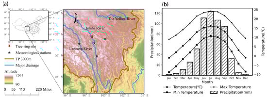
Figure 1.
(a) The specific location of the tree-ring sampling site and meteorological stations utilized in this research, along with (b) the average climatic factors (including the minimum temperature, the average temperature, the maximum temperature, and precipitation) for each month acquired at five meteorological stations from 1961 to 2016.
The sampling site is situated at the junction of Sichuan Province and the Tibet Autonomous Region within the southeastern Qinghai–Tibetan Plateau, along the Jinsha River (i.e., the section of the Yangtze River between Zhimenda and Pingshan; see Figure 1a). This region has a unique highland climate formed by the Tibetan Plateau’s topography and the synergistic effects of the South and East Asian monsoons and westward winds of the mid-latitudes. The extreme changes in climate are particularly evident here, with both the maximum and average temperatures increasing at a slower rate than the minimum temperature, and the warming rate increases with elevation [41]. It seems there is an increasingly positive correlation between extreme precipitation and overall rainfall, and precipitation intensifies in volume and frequency over time [42]. The increasing frequency of drought and frost phenomena and changes in the meteorological driving factors such as extreme weather have significantly affected vegetation growth in the study area [43]. Climate data from the study area (1961–2017) indicate an annual average temperature of 7.7 °C, with the highest average temperature of 16.2 °C in July and the lowest temperature of −1.1 °C in January. The average yearly precipitation was 568.1 mm, distributed in a single peak primarily between May and September, constituting 85.8% of the entire precipitation. The peak wet condition is in July, reaching up to 123.9 mm (Figure 1b). During sample collection, the collection object was older live trees. Increments borers were used to obtain two tree cores near the chest-high position of the trees, and one or three tree cores were collected for some trees. Ultimately, 61 cores were gathered from 37 trees.
All the sampled cores underwent preliminary processing following the globally recognized standard procedure for analyzing annual tree rings. With a measurement error rate of 0.01 mm, the LinTab™ system can be utilized to gauge the tree ring widths. The LinTab system is widely used in tree-ring width measurement due to its low data storage requirements and high resolution [44,45]. The cross-dating of rings was performed employing the COFECHA software [46]. In order to eliminate non-climatic data embedded within the original tree-ring widths, while preserving the maximum amount of climatic data, detrending was carried out using the ARSTAN program [47,48]. After multiple growth trend fittings using different methods, it was determined that the first-lowest filter method provided a better fit with the growth trend. This process yielded three standardized chronologies: Residual (RES), ARSTAN (ARS), and Standard (STD) chronologies. During the synthesis of the chronology, the individual sample cores that significantly deviated from the main series were excluded. The STD chronology was primarily employed for analyses in this research (all the following references to chronology are to the STD chronology, unless otherwise stated). The chronology spanned 663 years (1355–2017), with an average sensitivity of 0.188. The intra-tree and inter-tree correlation coefficients in the common interval between 1900 and 2000 were 0.562 and 0.327, respectively. Moreover, the signal-to-noise ratio (SNR), overall representativeness (expressed population signal, EPS), and proportion of variation described by the initial primary element were 0.964, 26.575, and 41.6%, respectively. These statistical characteristics imply that the chronology has a high average sensitivity and may represent climate changes in the past. To validate the reconstruction’s integrity, an EPS criterion of 0.85 was established to identify the period of reliable chronologies [49]. When the number of sample cores reached 12, the EPS exceeded 0.85, indicating a reliable time period from 1605 to 2017 (Figure 2).
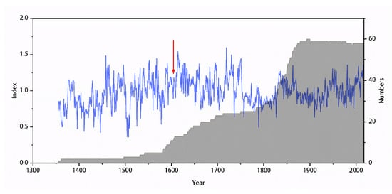
Figure 2.
The tree ring index and their count shows a red arrow highlighting the first year where the EPS exceeds a value of 0.85.
2.2. Climate Data
The climate data were sourced from five distinct stations: Dege County (98°35′ E, 31°48′ N, elevation 3184 m), Bainyu County (98°50′ E, 31°13′ N, elevation 3260 m), Batang County (99°6′ E, 30° N, elevation 2589.2 m), Changdu County (91°10′ E, 31°9′ N, elevation 3315 m), and Ganzi County (100° E, 31°37′, elevation 3393.5 m). These stations are geographically close to the sampling site (Figure 1a) and provided the minimum (Tmin) temperature, monthly mean (Tmean), maximum (Tmax), and precipitation (P) data from 1961 to 2016. In addition, the average values of these climatic factors from these sites were utilized to characterize the area’s weather. The global sea surface temperature (SST) data set (Extended Reconstructed Sea Surface Temperature V5, ERSST V5), with a spatial resolution of 2° × 2°, offered by NOAA, supplied the SST information. The sea surface temperature was used to examine the coupled air–sea interaction between the climate and the global SST in the study area.
2.3. Reconstruction and Analysis Methods
Pearson analysis could be employed to evaluate the linear correlations between the STD chronology and different climatic factors within the study region and to choose the primary climatic variables for reconstruction. While the traditional reconstruction methods primarily rely on constructing linear regression equations [50,51,52], the interplay between tree growth and climatic factors is highly complex and exhibits non-linear characteristics [53]. The previous studies have shown the efficacy of machine learning techniques in capturing non-linear regression relationships between tree growth and climatic factors [54,55,56]. Therefore, this study used three machine learning algorithms—K-nearest neighbors (KNNs), support vector machines (SVMs), and random forest (RF)—for modeling and reconstruction purposes. During the reconstruction process, chronological data from both the current and preceding years were employed for model training. This approach acknowledges the temperature’s lag effect on tree rings [57], indicating that the temperature in year t impacts the tree-ring widths both in that year and the next (year t + 1). The construction of machine learning algorithms was completed using the Python library package known as sklearn.
The accuracy and dependability of the reconstruction were evaluated through various statistical metrics, such as the correlation coefficient (R), the coefficient of determination (R2), the adjusted coefficient of determination (R2adj), error reduction (RE), the variance test (F), the product mean test, the sign test (ST), and the root-mean-square error (RMSE). To better understand extreme temperature variations, the temperature years were classified as high or low based on being one standard deviation (SD) above or below the mean. Years with reconstructed temperatures above the mean exceeding the SD (−4.08 °C) were identified as extremely high-temperature years, while years with reconstructed temperatures below the mean exceeding the SD (−5.2 °C) were classified as extremely low-temperature years. To further explain the decadal characteristics of the temperature shifts during the previous 411 years, analysis was conducted using the 11-year mean moving of the reconstruction. The phases in which the reconstruction results were lower or higher than the average for 10 consecutive years or more were defined as cold/warm phases.
The reconstructed and instrumental climate series were subjected to a spatial correlation analysis with the Climatic Research Unit (CRU TS 4.07) data set to gauge the spatial representativeness of the reconstructed minimum winter temperatures for the research region during the observational period from AD 1962 to 2005. To extract multi-timescale fluctuations from the reconstruction, ensemble empirical modal decomposition (EEMD) [58] was applied. EEMD decomposed the time series into various intrinsic modal functions (IMFs) with actual meanings, which extracted both time and frequency domain information from the amalgamated changes and trends [59]. Utilizing global sea surface temperature data, spatial correlation analysis was performed on the reconstruction and instrumental information to verify the influence of driving factors. The computation of the parameters for testing and the calculation of correlation coefficients were performed using both Python and SPSS software. The implementation of the Ensemble Empirical Mode Decomposition (EEMD) approach was also achieved using Python, and plotting was carried out using the matplotlib library in Python.
3. Results
3.1. Relationship between Tree Growth and Climate Factors
Figure 3 depicts the relationship between the tree-ring chronology and the regional climatic factors. The results imply that the radial growth of trees exhibits the most significant correlation with March and April precipitation, with correlation coefficients of 0.312 and 0.300, respectively (p < 0.05). Meanwhile, the correlation coefficient linking the trees’ radial growth and the Tmean in January, August, and November of the previous year, as well as the Tmax in February and August, were 0.287, 0.425, 0.314, 0.271, and 0.269, respectively (p < 0.05). A better correlation (p < 0.01) with the Tmean between this August and last December and between the Tmax in November and December of the previous year was found, with respective correlation coefficients of 0.425, 0.474, 0.391, and 0.433.
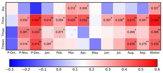
Figure 3.
The coefficients of the correlation between the tree-ring index and the climatic factors (pre, Tmin, Tmax, and Tmean indicate the monthly precipitation, minimum temperature, maximum temperature, and mean temperature, respectively). The statistical relationship of the tree-ring index with the climatic indicators, namely monthly precipitation (pre), and the trio of temperatures (minimum (Tmin), maximum (Tmax), and mean (Tmean)) is delineated by their correlation coefficients. Here, “Winter” represents the winter half-year (from last November to this April), and the correlation coefficients used are Pearson correlation coefficients. The symbols ** and * display the significance levels of 0.01 and 0.05, respectively.
The analysis of correlations for each individual month indicated that tree radial expansion was significantly associated (p < 0.05) with the minimum temperatures, with the exception of May in the current year. The most substantial correlation was observed with the average minimum temperature of the preceding December, boasting a correlation coefficient of 0.537 (p < 0.01). Through further correlation analysis of the climate elements of different month combinations, the correlation between the mean minimum temperature and the tree-ring chronology was found to pass the significance test at a level of significance of 0.01 in spring (March–April), high summer (August–September), and winter (last November–December and January in this year), and especially during the winter half-year (from last November to this April). The correlation coefficient of the winter half-year was the most significant, with its correlation coefficient reaching 0.566.
3.2. Minimum Temperature Reconstruction
In light of the aforementioned analysis, the average minimum temperature of the Jinsha River Basin during the winter half-year was selected as the object of reconstruction. Given the advantages of machine learning methods in modeling non-linear relationships, the present research incorporated three machine learning models, namely K-nearest neighbor (KNN), SVMs, and RF, in addition to the traditional regression equations for model construction.
The regression equation Lr (Tmin = 2.282 × stdt + 1.08 std(t+1) − 7.994) and the leave-one-out cross-validation (LOOCV) approach were employed to adjust the parameter of the machine learning model, and then the KNN, RF, and SVM models for temperature reconstruction were established. Ultimately, the reconstructed sequences obtained using the four methods were weighted and averaged with equal weights. Thus, an integrated reconstruction was obtained [60]. The correlation coefficient between the rebuilt and actual temperatures was 0.73 (with a sample size of 56, p < 0.001), and after accounting for degrees of freedom, the variance explained was 52.4% (as depicted in Figure 4a).
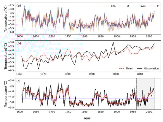
Figure 4.
(a) Comparison of four reconstruction results; (b) the constructed and observed temperatures during the calibration period of 1960–2016; and (c) the average minimum temperatures for the winter months reconstructed using the chronological data ranging from 1606 to 2016. The red line shows the moving average for 11 years, while the horizontal line signifies the average temperature across the entire reconstructed timeline.
To assess the robustness and dependability of the reconstruction model, a split-sample calibration/verification methodology was deployed for the ensemble reconstruction model. The segmented verification outcomes were consolidated and are presented in Table 1. Sign tests were conducted on both the initial data (ST) and the first-differenced data (ST1), and they successfully met the significance threshold at a level of 0.01, suggesting that the model has excellent reliability for the construction of both high- and low-frequency changes. The most stringent statistical reduction in error (RE) and coefficient of efficiency (CE) were positive; the RE values of the split calibration/verification test were much greater than 0, at 0.79 and 0.80, respectively.

Table 1.
Statistics of split calibration/verification test results for the tree-ring construction.
This suggests that the reconstruction outcomes are both stable and trustworthy, thereby validating their utility in reconstructing the average minimum winter half-year temperatures for the headwater of Jinsha River from 1606 to 2016. Furthermore, the reconstructed values of the average minimum winter half-year temperature exhibit a strong correlation with the observed values (Figure 4b) and the correlation coefficient of 0.730 (n = 56, p < 0.01).
3.3. Characteristic Changes in Minimum Temperature
As shown in Figure 4c, the fluctuations in the average minimum temperature during the wintertime in the year exhibited marked variations during the last 411 years (between 1606 and 2016), and the mean of the reconstructed minimum temperature (−4.64 °C) was lower than the observed temperature in the instrumental period (−4.57 °C, 1961–2016). The reconstructed temperature varied from −5.47 °C (in 1880) to −3.17 °C (in 1719), with a standard deviation (SD) of 0.56 °C. In the last 411 years, there have been 80 years of exceptionally high temperatures and 92 years of exceptionally low temperatures, constituting 19.4% and 22.4%, respectively. Notably, the periods of 1755–1759, 1775–1779, 1795–1805, and 1813–1817 were characterized by consecutive and persistent extremely low-temperature phases lasting five or more years, while the periods of 1610–1618, 1626–1630, 1693–1697, 1725–1734, 1742–1751, and 2010–2016 experienced sustained extreme high temperatures for five or more consecutive years.
In the last 411 years, the study area has experienced six cold and seven warm phases. The cold periods occurred during 1663–1672, 1702–1712, 1754–1829, 1869–1942, 1959–1979, and 1985–1994. The warm periods, on the other hand, were observed in 1611–1662, 1673–1701, 1713–1753, 1830–1852, 1858–1868, 1943–1958, and 1995–2011.
4. Discussion
4.1. Response of the Radial Growth of Tree Rings to Meteorological Elements
The examination of the relationship between the tree-ring width chronologies and meteorological variables showed the radial tree growth within the study region was more responsive to temperature fluctuations compared to fluctuations in the rainfall levels. The Tmin value of the winter half-year might be the primary influence on tree growth. This finding aligns with the outcomes of previous research conducted in neighboring regions [33,61], the lower Yangtze River [62], and southern Poland [63]. An excessive Tmin in a given winter half-year would result in the condensation of ice crystals, disrupting the vesicles and leading to cellular dehydration, which would cause permanent damage to the tree root tissues, subsequently affecting tree growth in the following growing season [64]. Additionally, colder winters may lead to permafrost layer thickening, which would impede water uptake and cause winter drying.
In conclusion, the prospects for tree growth in the ensuing year are anticipated to decrease [65]. Furthermore, a thicker permafrost delays the snowmelt date as well as the onset of the season of tree growing season, limiting their growth and development [28]. Conversely, warmer winters could reduce the consumption of stored carbohydrates by trees to maintain physiological activities. This favorable condition promotes tree growth and development in the upcoming year. Specifically, spruce might exhibit significant photosynthesis during warm winters, which ensures sufficient nutrient availability for the subsequent growing season, thus facilitating the growth of spring timber [23]. These explanations shed light on why the radial growth of spruce in the Jinsha River Basin is affected by low winter temperatures.
4.2. Temporal Representativeness and Reconstruction Reliability
To further evaluate the accuracy of this reconstruction on longer timescales before the instrumental period and the representativeness of large spatial scales utilizing the reconstructed and observed minimum winter temperatures, we conducted spatial correlation analysis with the Climatic Research Unit time series (CRU) gridded data set (TS 4.07). The spatial correlation outcomes revealed analogous patterns between the observed (Figure 5a) and reconstructed (Figure 5b) temperature data. Although the observed data exhibited stronger correlations, both data sets demonstrated significant correlations with the CRU gridded surface temperature data within the area. This indicates that the reconstructed results are representative of the climate fluctuations within the study region and its adjacent regions.
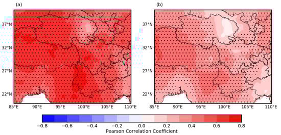
Figure 5.
The spatial correlations between the observed (a) and reconstructed (b) minimum winter temperatures of the southeastern Tibetan Plateau were assessed against the winter gridded temperatures provided by the Climatic Research Unit (CRU TS 4.07) for the period from 1962 to 2016. The stippled areas indicate statistical significance at the p < 0.01 level.
The reconstructed series were juxtaposed with the temperature reconstructions from nearby places, encompassing winter temperatures of the southeastern Tibetan Plateau during the last 1340 years [27], the reconstruction of warm season temperatures in the southeastern Tibetan Plateau for the previous 449 years [30], and the reconstructed minimum winter temperatures in the western Sichuan Plateau from 1650 to 1994 [66]. The reconstructed temperatures exhibit a significant level of agreement with each other, as indicated by the correlation coefficients of 0.298 (n = 359, p < 0.01), 0.279 (n = 407, p < 0.01), and 0.304 (n = 345, p < 0.01) in the common periods. The warm and cold changes were comparatively analyzed using an 11-year sliding average and Z-score normalization for all the sequences (Figure 6). Despite variations across the reconstructed temporal segments and variables studied, the synchronization of warm and cold changes among the four temperature reconstructions remained consistent, further evidencing the reliability of the results. The reconstructed temperature results share warm and cold periods, including a span of warmer conditions in the 1610s, an interval characterized by cooler temperatures in the 1740s, a stretch of colder climatic conditions in the early 1900s, a phase of elevated thermal conditions in the 1950s, and an interval marked by increased warmth in the late 1900s. In addition, the cold phase of the early 18th century, the warm phase of the 1710s, the cold phase of the early 19th century, the cold phase of the 1850s, and the cold phase of the 1960s are represented among several reconstructions (including the reconstruction of the present study). Some of the disparities observed in the warm and cold phases across the four reconstructions can likely be ascribed to a variety of causes. These include the specific objects of reconstruction (varying meteorological elements), the distinct time periods chosen for the reconstructions, the methodologies applied for detrending the data, as well as the geographical demarcation and categorization of the study area. The interplay of these elements may jointly contribute to the differences noted in the reconstruction outcomes.
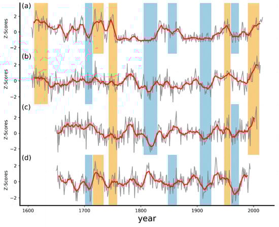
Figure 6.
Comparison of the winter minimum temperature reconstruction in this research (a), the winter temperature reconstruction of the southeastern Tibetan Plateau [27] (b), the reconstruction of the warm period temperatures in the southeastern Tibetan Plateau [30] (c), and the reconstructed minimum winter temperatures in the western Sichuan Plateau [66] (d). The regions with shading signify the durations when the reconstructions align in their trend movements.
In addition, the reconstructed temperature that occurred during the cold phase in the 1900s was confirmed in the work on temperature reconstruction using ice cores taken from the Tibetan Plateau [67]. The reconstructed temperature aligns well with the cold winters of 1875–1880, 1890, 1920, and 1980, as indicated by the European instrumental record [63]. The oscillations in the reconstruction correspond to the advancement and retreat of glaciers in the Tibetan Plateau region. Notably, the reconstructed temperatures experienced a period of significant cooling and persistent cold from 1748 to 1767, coinciding with the largest glacier advance event since the Little Ice Age in the Middushu Ice, located in the western Tibetan Plateau. This result is corroborated by the validation of the most extensive and peripheral moraines, which occurred around 1767 [68]. In addition, the reconstructed temperatures demonstrated a notable cooling trend before 1880, which corresponds to a clear progression of glacial activity in the Trans-Himalayan region [69]. Furthermore, the reconstruction between 1790 and 1820 indicates a significant period of low temperatures, which is called the Dalton Minimum, at the transition between the 18th and 19th centuries. This cold period was affected by changes in solar irradiance, volcanic activity (e.g., the 1815 eruption of the Tambora volcano in Indonesia), and rising CO2 concentrations. These factors resulted in a sudden drop in temperatures not only in the Northern Hemisphere, but even globally, with reports of a summer-free year [70,71]. Moreover, a sustained cooling trend from 1860 to 1880 was documented in the Western Himalayan region [24]. The reconstruction captured signs of rapid warming on the Tibetan Plateau during the last fifty years in the 1900s, indicating a direct temperature increase at a rate of 0.2 °C during the last five decades. These findings match the conclusions drawn from climate reconstruction efforts using tree rings [72,73,74]. It merits particular attention that some paleoclimate findings in the Northern Hemisphere show temperature discrepancies, which are attributed to issues related to tree-ring dispersion [75]. However, the reconstructions in this study retain temperature sensitivity, and the increase in the reconstructed temperatures align with the warming trends observed in the instrumental data.
It is intriguing to observe that the relatively “warm period” of the study area on the centennial timescale is clearly different from the notion of a “cool period” (Little Ice Age) during this time, with the Tmin of the half-year wintertime in the research region during 1650–1750 being superior to those of the 20th century by approximately 0.44 °C. Despite being in the Maunder minimum, apparent warming in the 17th century was not an isolated phenomenon, and this has been reported in climate reconstructions using tree rings and ice cores in the Tibetan Plateau region [27,76,77]. The reconstruction findings of the cold season temperature changes in the northeastern Qinghai–Tibet Plateau using alkene ketone also indicate that the chilly seasons of the Little Ice Age were not the coldest periods, aligning with the findings of this research [78]. This phenomenon is not unique to some regions of the Tibetan Plateau, but also occurred in North America across the ocean [25,79,80].
A plausible rationale for this phenomenon is that an augmented pressure gradient between south-central Asia and northern Eurasia could potentially intensify the westerlies in the mid-latitude regions, preventing cold air from moving southward toward the Tibetan Plateau [81].
4.3. Reconstructing Multiscale Fluctuations in Temperature
Considering that long-term climate evolution is usually non-stationary and non-linear and occurs at multiple timescales, to extract the available climate change signals and explore the cyclic changes in the extrinsic forcing of the minimum temperature during the winter semester, the authors of this paper used the Ensemble Empirical Mode Decomposition (EEMD) approach to break down the reconstruction at multiple scales (Figure 7). A total of six IMFs (IMFs 1–6) were obtained using EEMD that could characterize the fluctuations in the reconstruction from high-frequency to low-frequency scales, and each mode contains information with an actual physical meaning (Table 2).
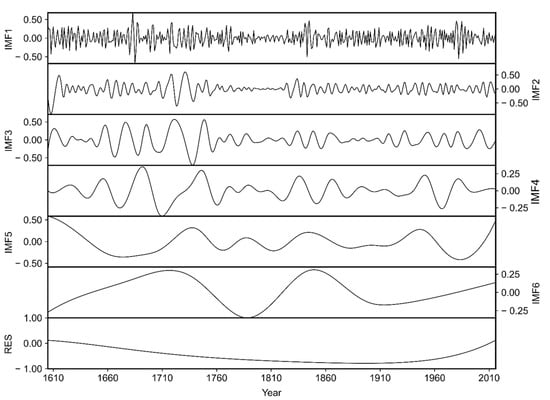
Figure 7.
Extracted components of reconstructed minimum winter half-year temperatures using Ensemble Empirical Mode Decomposition.
Table 2.
Contributions to the variance and coefficient of reconstruction after the EEMD of IMFs and trends (RES).
The reconstructed temperatures had relatively invariant intervals characterized by high-frequency temporal dynamics, with major periods of 3.3–3.4 and 7.1–7.4 years for IMF1 and IMF2, respectively. The results align with the periods (2–8a) of the El Niño–Southern Oscillation (ENSO), suggesting that large-scale coupled sea–air oscillations have an important influence on the variation in the winter minimum temperatures within the purview of this research locale, which has been documented in the existing body of research [82]. During the El Niño years of the ENSO cycle, an anomalous anticyclone located in the western troposphere of the Pacific Ocean weakened the strength of the East Asian Winter Monsoon (EAWM). This could cause significantly higher-than-average winter surface temperatures in most parts of China, while in the La Niña years, the situation was reversed, and such temperature anomalies would persist into the following spring or even early summer [83]. Nevertheless, the spatial correlation assessment of the reconstructed and empirically obtained temperatures during the global winter half-year (P11C4) SST (Figure 8a,b) indicates that the correlation between the SST and the reconstructed and observed temperatures in the El Niño Sea area is insignificant (p > 0.05). However, there is better agreement between the Indian Ocean and the western and central parts of the mid-latitude Pacific Ocean. The bridging anomalous anticyclone of ENSO influencing the winter temperatures in East Asia is profoundly influenced by the evolution of SST anomalies in the equatorial western Pacific Ocean, and the anomalous cooling of SSTs in this region directly affect the Rossby waves within the lower stratum of the troposphere, which, in turn, affect the strength of the anomalous anticyclone [84]. Meanwhile, the influence of ENSO on the climate of East Asia is also regulated by the SST of the Indian Ocean, and the anomalous enhancement of the anticyclone anomaly in the western North Pacific Ocean occurs when the El Niño phenomenon exists concurrently with the affirmative phase of the Indian Ocean dipole sub-mode [85]. The aforementioned mechanism helps elucidate the distribution of the regions where the winter half-year temperature and the global SST were significantly correlated.
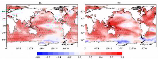
Figure 8.
Spatial correlations of reconstructed (a) and observed (b) minimum winter half-year temperatures with SST data during the period of 1845–2016 and during the period of 1961–2016, respectively. The 95% confidence interval is shown by the dotted region.
The variation in the 15.5–16.8-year cycle of IMF3 might be indicative of Pacific Decadal Oscillation (PDO), which is an important component of the North Pacific SST anomalies, and its influence covers the North Pacific SST and even the global climate [86]. The correlation coefficient between the reconstruction and the PDO was 0.295 (1606–1996, n = 391, p < 0.001). The interplay between Pacific Decadal Oscillation (PDO) and the atmospheric circulation patterns suggests a robust inverse pressure correlation between these two elements over the North Pacific Ocean and eastern China. When the PDO entered its positive (negative) phase, there was a corresponding decrease (increase) in sea level pressure within the mid- to high-latitude regions of East Asia and the North Pacific. The potency of the Siberian high-pressure system decreased (elevated), and the upper-level latitudinal winds weakened (strengthened), which, in turn, led to warmer (colder) winters in China [87]. The sunspot cycle (Schwabe) was around 11 years, which corresponds to the cycle of IMF4 in this paper (multiples of 11a). The effect of solar activity on anthropogenic climate alteration has been verified in numerous climate reconstructions employing tree-ring width chronologies [30,31,88].
The quasi-82a period of IMF5 could potentially correlate with Atlantic Multidecadal Oscillation (AMO), an inter-decadal variation in the SST over a period of 60–80 years, as observed in various studies conducted in the Tibetan Plateau region [29,61]. The IMF6 component, which represents temperature variation in the reconstructed sequence on a multi-hundred-year scale, had a weaker oscillation and corresponds to an extrinsic driver, which might be the same as the AMO (quasi-multiples of 80 years). The correlation coefficient between the IMF5 and the AMO index during 1871–2016 is 0.518 (n = 146, p < 0.001). As an oceanic model, the AMO regulates the surface air pressure and temperature through atmospheric conduits extending from the Atlantic Ocean, encompassing westerly winds and the associated wave train. The westerlies are influenced by the large topography of the Tibetan Plateau and separated into several branches, whose southern branch reaches southwestern China and moderates the winter air temperatures in the region [89]. Meanwhile, the AMO is strongly related to the interdecadal variations of the East Asian Monsoon. Research has found that the positive (warm) phase of the AMO aligns with a period of weak EAWM in most of China, having relatively warm winters, and vice versa, which corresponds to winters with cooler temperatures [90].
Spatial correlation analysis was conducted on both the reconstructed temperature sequence from 1845 to 2016 and the instrumental record from 1961 to 2016, and each correlate with the global sea surface temperatures (SSTs) from the previous November to this April, as illustrated in Figure 8a,b. This analysis effectively validated the role of sea–air coupling patterns as driving factors within the climate system. The differences in the measured lowest temperature at regional meteorological stations are both synchronized with the fluctuations in the SST, in which there are more regions of significant positive correlation (p < 0.05) between the reconstructed sequences and the SST than instrumental sequences. The overall correlation between the observed temperature and the SST is slightly higher than that of the reconstructed temperature. The synergistic relationship between the minimum temperature during the winter semester and the SSTs in the western Pacific, Indian, North Atlantic, South Atlantic, and Arctic Oceans in the study area further demonstrate the association between thermal fluctuations within the region and the synergistic factors of the air and sea. The specific mechanisms of the influence warrant further research.
5. Conclusions
A standardized chronology of tree-ring width was formulated utilizing spruce from the Jinsha River Basin, and the regional mean minimum temperatures recorded during the winter semester were reconstructed for the period from 1606 to 2016. The reconstruction recorded stronger decadal variations, reflecting six cold periods and seven warm periods. The reconstructed temperature, when compared with those from the neighboring areas, was discovered to consistently reveal warm and cold epochs. Additionally, the reconstruction results from other proxies, meteorological data recorded by early instruments, and historical data on the timing of glacial activity and natural disasters also support the dependability of the reconstruction results. The reconstruction sensitively captures the climate warming observed during the last 50 years in the 1900s. Unexpectedly, the recorded tree-ring data showed that the research region was relatively warm in the winter half-years from the 17th to 18th century, but should have been cold during the Little Ice Age. This phenomenon of the “warm winter of the Little Ice Age” is also supported by other winter temperature reconstructions. The winter half-year minimum temperatures could be affected by the El Niño–Southern Oscillation (ENSO), Pacific Decadal Oscillation (PDO), solar activity, and Atlantic Multidecadal Oscillation (AMO). In this study, the integration of several reconstruction methods was performed, and temperature’s hysteresis influence on tree rings was considered, providing a new idea for reconstruction work. In future research, the reconstructed temperature should be supplemented with high-resolution meteorological data and sufficient sample sizes in more areas in order to more effectively address the challenges posed by global climate change.
Author Contributions
Conceptualization, J.L.; methodology, J.L. and C.J.; software, J.L., C.J. and Y.T.; validation, J.L. and H.X.; formal analysis, J.L.; investigation, J.L.; resources, J.L.; data curation, J.L. and C.J.; writing—original draft preparation, C.J. and H.X.; writing—review and editing, J.L.; visualization, C.J. and Y.T.; supervision, J.L.; project administration, J.L.; funding acquisition, J.L. All authors have read and agreed to the published version of the manuscript.
Funding
This research was jointly funded by the Second Tibetan Plateau Scientific Expedition and Research (STEP) program (No. 2019QZKK0103 and 2019QZKK0608), the Natural Science Foundation of Sichuan Province (No. 2022NSFSC0215), and the Undergraduate Innovation and Entrepreneurship Training Program (No. 202310621007).
Data Availability Statement
The data of this study are available upon request to the first or corresponding author.
Conflicts of Interest
The authors declare no conflicts of interest.
References
- Fang, J.; Zhu, J.; Wang, S.; Yue, C.; Shen, H. Global Warming, Human-Induced Carbon Emissions, and Their Uncertainties. Sci. China Earth Sci. 2011, 54, 1458–1468. [Google Scholar] [CrossRef]
- Boyles, R.P.; Raman, S. Analysis of Climate Trends in North Carolina (1949–1998). Environ. Int. 2003, 29, 263–275. [Google Scholar] [CrossRef]
- Liu, X.; Chen, B. Climatic Warming in the Tibetan Plateau during Recent Decades. Int. J. Climatol. 2000, 20, 1729–1742. [Google Scholar] [CrossRef]
- Huang, J.; Guan, X.; Ji, F. Enhanced Cold-Season Warming in Semi-Arid Regions. Atmos. Chem. Phys. 2012, 12, 5391–5398. [Google Scholar] [CrossRef]
- Schwartz, M.D.; Ahas, R.; Aasa, A. Onset of Spring Starting Earlier across the Northern Hemisphere. Glob. Change Biol. 2006, 12, 343–351. [Google Scholar] [CrossRef]
- Piao, S.; Friedlingstein, P.; Ciais, P.; Viovy, N.; Demarty, J. Growing Season Extension and Its Impact on Terrestrial Carbon Cycle in the Northern Hemisphere over the Past 2 Decades. Glob. Biogeochem. Cycles 2007, 21, 2006GB002888. [Google Scholar] [CrossRef]
- Brooks, P.D.; Grogan, P.; Templer, P.H.; Groffman, P.; Öquist, M.G.; Schimel, J. Carbon and Nitrogen Cycling in Snow-Covered Environments: Carbon and Nitrogen Cycling in Snow-Covered Environments. Geogr. Compass 2011, 5, 682–699. [Google Scholar] [CrossRef]
- Cai, Q.; Liu, Y.; Wang, Y.; Ma, Y.; Liu, H. Recent Warming Evidence Inferred from a Tree-Ring-Based Winter-Half Year Minimum Temperature Reconstruction in Northwestern Yichang, South Central China, and Its Relation to the Large-Scale Circulation Anomalies. Int. J. Biometeorol. 2016, 60, 1885–1896. [Google Scholar] [CrossRef]
- Xiong, Y.; Zhou, J.; Sun, N.; Jia, B.; Hu, G. Variation Trends of Precipitation and Runoff in the Jinsha River Basin, China: 1961–2015. IOP Conf. Ser. Earth Environ. Sci. 2020, 440, 052044. [Google Scholar] [CrossRef]
- He, Y.; Zhang, Y.; Wu, Z. Analysis of Climate Variability in the Jinsha River Valley. J. Trop. Meteorol. 2016, 22, 243–251. [Google Scholar] [CrossRef]
- Zhang, D.; Wang, W.; Liang, S.; Wang, S. Spatiotemporal Variations of Extreme Precipitation Events in the Jinsha River Basin, Southwestern China. Adv. Meteorol. 2020, 2020, 3268923. [Google Scholar] [CrossRef]
- Liu, X.; Peng, D.; Xu, Z. Identification of the Impacts of Climate Changes and Human Activities on Runoff in the Jinsha River Basin, China. Adv. Meteorol. 2017, 2017, 4631831. [Google Scholar] [CrossRef]
- Schwartz, S.A. An Interdisplinary Approach to the Little Ice Age and Its Implications for Global Change Research. Ph.D. Thesis, University of Michigan, Ann Arbor, MI, USA, 1994. [Google Scholar]
- Wang, S.; Liu, J.; Zhou, J. The Climate of Little Ice Age Maximum in China. Lake Sci. 2015, 15, 369–376. [Google Scholar] [CrossRef][Green Version]
- Felis, T.; Ionita, M.; Rimbu, N.; Lohmann, G.; Kölling, M. Mild and Arid Climate in the Eastern Sahara-Arabian Desert During the Late Little Ice Age. Geophys. Res. Lett. 2018, 45, 7112–7119. [Google Scholar] [CrossRef]
- Pitman, K.J.; Smith, D.J. Tree-Ring Derived Little Ice Age Temperature Trends from the Central British Columbia Coast Mountains, Canada. Quat. Res. 2012, 78, 417–426. [Google Scholar] [CrossRef]
- Shen, D.; Li, S. Environment Change of Sihu Lake in the Past 450 Years, Southern China. Environ. Earth Sci. 2013, 70, 2953–2962. [Google Scholar] [CrossRef]
- Jomelli, V.; Lane, T.; Favier, V.; Masson-Delmotte, V.; Swingedouw, D.; Rinterknecht, V.; Schimmelpfennig, I.; Brunstein, D.; Verfaillie, D.; Adamson, K.; et al. Paradoxical Cold Conditions during the Medieval Climate Anomaly in the Western Arctic. Sci. Rep. 2016, 6, 32984. [Google Scholar] [CrossRef]
- Degroot, D. Climate Change and Society in the 15th to 18th Centuries. WIREs Clim. Chang. 2018, 9, e518. [Google Scholar] [CrossRef]
- Yang, B.; Braeuning, A.; Liu, J.; Davis, M.E.; Yajun, S. Temperature Changes on the Tibetan Plateau during the Past 600 Years Inferred from Ice Cores and Tree Rings. Glob. Planet. Change 2009, 69, 71–78. [Google Scholar] [CrossRef]
- Nesje, A.; Dahl, S.O.; Thun, T.; Nordli, O. The “Little Ice Age” Glacial Expansion in Western Scandinavia: Summer Temperature or Winter Precipitation? Clim. Dyn. 2008, 30, 789–801. [Google Scholar] [CrossRef]
- Chen, F.; Yuan, Y.; Wei, W.; Yu, S.; Zhang, T. Tree Ring-Based Winter Temperature Reconstruction for Changting, Fujian, Subtropical Region of Southeast China, since 1850: Linkages to the Pacific Ocean. Theor. Appl. Climatol. 2012, 109, 141–151. [Google Scholar] [CrossRef]
- Shah, S.K.; Pandey, U.; Mehrotra, N.; Wiles, G.C.; Chandra, R. A Winter Temperature Reconstruction for the Lidder Valley, Kashmir, Northwest Himalaya Based on Tree-Rings of Pinus Wallichiana. Clim. Dyn. 2019, 53, 4059–4075. [Google Scholar] [CrossRef]
- Borgaonkar, H.P.; Ram, S.; Sikder, A.B. Assessment of Tree-Ring Analysis of High-Elevation Cedrus Deodara D. Don from Western Himalaya (India) in Relation to Climate and Glacier Fluctuations. Dendrochronologia 2009, 27, 59–69. [Google Scholar] [CrossRef]
- Porter, T.J.; Pisaric, M.F.J.; Field, R.D.; Kokelj, S.V.; Edwards, T.W.D.; deMontigny, P.; Healy, R.; LeGrande, A.N. Spring-Summer Temperatures since AD 1780 Reconstructed from Stable Oxygen Isotope Ratios in White Spruce Tree-Rings from the Mackenzie Delta, Northwestern Canada. Clim. Dyn. 2014, 42, 771–785. [Google Scholar] [CrossRef][Green Version]
- Wang, L.; Duan, J.; Chen, J.; Huang, L.; Shao, X. Temperature Reconstruction from Tree-ring Maximum Density of Balfour Spruce in Eastern Tibet, China. Int. J. Climatol. 2010, 30, 972–979. [Google Scholar] [CrossRef]
- Huang, R.; Zhu, H.; Liang, E.; Liu, B.; Shi, J.; Zhang, R.; Yuan, Y.; Grießinger, J. A Tree Ring-Based Winter Temperature Reconstruction for the Southeastern Tibetan Plateau since 1340 CE. Clim. Dyn. 2019, 53, 3221–3233. [Google Scholar] [CrossRef]
- Gou, X.; Chen, F.; Jacoby, G.; Cook, E.; Yang, M.; Peng, J.; Zhang, Y. Rapid Tree Growth with Respect to the Last 400 Years in Response to Climate Warming, Northeastern Tibetan Plateau. Int. J. Climatol. 2007, 27, 1497–1503. [Google Scholar] [CrossRef]
- Liang, E.; Shao, X.; Qin, N. Tree-Ring Based Summer Temperature Reconstruction for the Source Region of the Yangtze River on the Tibetan Plateau. Glob. Planet. Change 2008, 61, 313–320. [Google Scholar] [CrossRef]
- Duan, J.; Zhang, Q.-B. A 449 Year Warm Season Temperature Reconstruction in the Southeastern Tibetan Plateau and Its Relation to Solar Activity: Temperature Reconstruction in the Tibet. J. Geophys. Res. Atmos. 2014, 119, 11578–11592. [Google Scholar] [CrossRef]
- Gou, X.; Gao, L.; Deng, Y.; Chen, F.; Yang, M.; Still, C. An 850-year Tree-ring-based Reconstruction of Drought History in the Western Qilian Mountains of Northwestern China. Int. J. Climatol. 2015, 35, 3308–3319. [Google Scholar] [CrossRef]
- Deng, Y.; Gou, X.; Gao, L.; Yang, T.; Yang, M. Early-Summer Temperature Variations over the Past 563 Yr Inferred from Tree Rings in the Shaluli Mountains, Southeastern Tibet Plateau. Quat. Res. 2014, 81, 513–519. [Google Scholar] [CrossRef]
- Li, J.; Li, J.; Li, T.; Au, T.F. 351-Year Tree Ring Reconstruction of the Gongga Mountains Winter Minimum Temperature and Its Relationship with the Atlantic Multidecadal Oscillation. Clim. Chang. 2021, 165, 49. [Google Scholar] [CrossRef]
- Chen, F.; Shang, H.; Panyushkina, I.P.; Meko, D.M.; Yu, S.; Yuan, Y.; Chen, F. Tree-Ring Reconstruction of Lhasa River Streamflow Reveals 472 Years of Hydrologic Change on Southern Tibetan Plateau. J. Hydrol. 2019, 572, 169–178. [Google Scholar] [CrossRef]
- Li, T.; Li, J. A 564-Year Annual Minimum Temperature Reconstruction for the East Central Tibetan Plateau from Tree Rings. Glob. Planet. Change 2017, 157, 165–173. [Google Scholar] [CrossRef]
- Li, Z.-S.; Zhang, Q.-B.; Ma, K. Tree-Ring Reconstruction of Summer Temperature for A.D. 1475–2003 in the Central Hengduan Mountains, Northwestern Yunnan, China. Clim. Change 2012, 110, 455–467. [Google Scholar] [CrossRef]
- Gou, X.; Yang, T.; Gao, L.; Deng, Y.; Yang, M.; Chen, F. A 457-Year Reconstruction of Precipitation in the Southeastern Qinghai-Tibet Plateau, China Using Tree-Ring Records. Chin. Sci. Bull. 2013, 58, 1107–1114. [Google Scholar] [CrossRef]
- Fan, Z.; Bräuning, A.; Cao, K. Tree-ring Based Drought Reconstruction in the Central Hengduan Mountains Region (China) since A.D. 1655. Int. J. Climatol. 2008, 28, 1879–1887. [Google Scholar] [CrossRef]
- Yang, B.; Chen, X.; He, Y.; Wang, J.; Lai, C. Reconstruction of Annual Runoff since CE 1557 Using Tree-Ring Chronologies in the Upper Lancang-Mekong River Basin. J. Hydrol. 2019, 569, 771–781. [Google Scholar] [CrossRef]
- Xiao, D.; Shao, X.; Qin, N.; Huang, X. Tree-Ring-Based Reconstruction of Streamflow for the Zaqu River in the Lancang River Source Region, China, over the Past 419 Years. Int. J. Biometeorol. 2017, 61, 1173–1189. [Google Scholar] [CrossRef]
- Yao, L.; Lu, J.; Zhang, W.; Qin, J.; Zhou, C.; Ngoc, N.T.; Pinage, E.R. Spatiotemporal Analysis of Extreme Temperature Change on the Tibetan Plateau Based on Quantile Regression. Earth Space Sci. 2022, 9, e2022EA002571. [Google Scholar] [CrossRef]
- Ge, G.; Shi, Z.; Yang, X.; Hao, Y.; Guo, H.; Kossi, F.; Xin, Z.; Wei, W.; Zhang, Z.; Zhang, X.; et al. Analysis of Precipitation Extremes in the Qinghai-Tibetan Plateau, China: Spatio-Temporal Characteristics and Topography Effects. Atmosphere 2017, 8, 127. [Google Scholar] [CrossRef]
- Valjarevic, A.; Popovici, C.; Stilic, A.; Radojkovic, M. Cloudiness and Water from Cloud Seeding in Connection with Plants Distribution in the Republic of Moldova. Appl. Water Sci. 2022, 12, 262. [Google Scholar] [CrossRef]
- Maes, S.L.; Vannoppen, A.; Altman, J.; Van Den Bulcke, J.; Decocq, G.; De Mil, T.; Depauw, L.; Landuyt, D.; Perring, M.P.; Van Acker, J.; et al. Evaluating the Robustness of Three Ring-Width Measurement Methods for Growth Release Reconstruction. Dendrochronologia 2017, 46, 67–76. [Google Scholar] [CrossRef]
- Ziemiańska, M.; Kalbarczyk, R. Biometrics of Tree-Ring Widths of (Populus X Canadensis Moench) and Their Dependence on Precipitation and Air Temperature in South-Western Poland. Wood Res. 2018, 63, 2018. [Google Scholar]
- Holmes, R.L. Computer-Assisted Quality Control in Tree-Ring Dating and Measurement. Tree-Ring Bull 1983, 43, 51–67. [Google Scholar] [CrossRef]
- Cook, E.R. A Time Series Analysis Approach to Tree Ring Standardization; Dendrochronology, Forestry, Dendroclimatology, Autoregressive Process: Tucson, AZ, USA, 1985. [Google Scholar]
- Cook, E.; Briffa, K. A Comparison of Some Tree-Ring Standardization Methods. In Methods of Dendrochronology; Cook, E.R., Kairiukstis, L.A., Eds.; Applications in the Environmental Sciences: Boston, MA, USA, 1990. [Google Scholar]
- Choi, E.-B.; Sano, M.; Park, J.-H.; Kim, Y.-J.; Li, Z.; Nakatsuka, T.; Hakozaki, M.; Kimura, K.; Jeong, H.-M.; Seo, J.-W. Synchronizations of Tree-Ring δ18O Time Series within and between Tree Species and Provinces in Korea: A Case Study Using Dominant Tree Species in High Elevations. J. Wood Sci. 2020, 66, 53. [Google Scholar] [CrossRef]
- Wang, Y.; Feng, Q.; Kang, X. Tree-Ring-Based Reconstruction of Temperature Variability (1445–2011) for the Upper Reaches of the Heihe River Basin, Northwest China. J. Arid Land 2016, 8, 60–76. [Google Scholar] [CrossRef]
- Yang, B.; Kang, X.; Braeuning, A.; Liu, J.; Qin, C.; Liu, J. A 622-Year Regional Temperature History of Southeast Tibet Derived from Tree Rings. Holocene 2010, 20, 181–190. [Google Scholar] [CrossRef]
- Tian, Q.; Gou, X.; Zhang, Y.; Peng, J.; Wang, J.; Chen, T. Tree-Ring Based Drought Reconstruction (A.D. 1855–2001) for the Qilian Mountains, Northwestern China. Tree-Ring Res. 2007, 63, 27–36. [Google Scholar] [CrossRef]
- Khan, N.; Sachindra, D.A.; Shahid, S.; Ahmed, K.; Shiru, M.S.; Nawaz, N. Prediction of Droughts over Pakistan Using Machine Learning Algorithms. Adv. Water Resour. 2020, 139, 103562. [Google Scholar] [CrossRef]
- Lin, Y.; Salekin, S.; Meason, D.F. Modelling Tree Diameter of Less Commonly Planted Tree Species in New Zealand Using a Machine Learning Approach. Forestry 2023, 96, 87–103. [Google Scholar] [CrossRef]
- Jevšenak, J.; Džeroski, S.; Levanič, T. Predicting the Vessel Lumen Area Tree-Ring Parameter of Quercus Robur with Linear and Nonlinear Machine Learning Algorithms. Geochronometria 2018, 45, 211–222. [Google Scholar] [CrossRef]
- Zhang, H.; Feng, Z.; Wang, S.; Ji, W. Disentangling the Factors That Contribute to the Growth of Betula spp. and Cunninghami Lanceolata in China Based on Machine Learning Algorithms. Sustainability 2022, 14, 8346. [Google Scholar] [CrossRef]
- Briffa, K.R.; Jones, P.D.; Bartholin, T.S.; Eckstein, D.; Schweingruber, F.H.; Karlén, W.; Zetterberg, P.; Eronen, M. Fennoscandian Summers from Ad 500: Temperature Changes on Short and Long Timescales. Clim. Dyn. 1992, 7, 111–119. [Google Scholar] [CrossRef]
- Shi, F.; Yang, B.; Von Gunten, L.; Qin, C.; Wang, Z. Ensemble Empirical Mode Decomposition for Tree-Ring Climate Reconstructions. Theor. Appl. Climatol. 2012, 109, 233–243. [Google Scholar] [CrossRef]
- Yin, H.; Liu, H.; Linderholm, H.W.; Sun, Y. Tree Ring Density-Based Warm-Season Temperature Reconstruction since A.D. 1610 in the Eastern Tibetan Plateau. Palaeogeogr. Palaeoclimatol. Palaeoecol. 2015, 426, 112–120. [Google Scholar] [CrossRef]
- Zhao, X.; Fang, K.; Chen, F.; Martín, H.; Roig, F.A. Reconstructed Jing River Streamflow from Western China: A 399-Year Perspective for Hydrological Changes in the Loess Plateau. J. Hydrol. 2023, 621, 129573. [Google Scholar] [CrossRef]
- Shi, S.; Li, J.; Shi, J.; Zhao, Y.; Huang, G. Three Centuries of Winter Temperature Change on the Southeastern Tibetan Plateau and Its Relationship with the Atlantic Multidecadal Oscillation. Clim. Dyn. 2017, 49, 1305–1319. [Google Scholar] [CrossRef]
- Shi, J.; Cook, E.; Lu, H.; Li, J.; Wright, W.; Li, S. Tree-Ring Based Winter Temperature Reconstruction for the Lower Reaches of the Yangtze River in Southeast China. Clim. Res. 2010, 41, 169–176. [Google Scholar] [CrossRef]
- Opała, M.; Mendecki, M.J. An Attempt to Dendroclimatic Reconstruction of Winter Temperature Based on Multispecies Tree-Ring Widths and Extreme Years Chronologies (Example of Upper Silesia, Southern Poland). Theor. Appl. Climatol. 2014, 115, 73–89. [Google Scholar] [CrossRef]
- Körner, C. A Re-Assessment of High Elevation Treeline Positions and Their Explanation. Oecologia 1998, 115, 445–459. [Google Scholar] [CrossRef]
- Körner, C. Alpine Treelines; Springer: Basel, Switzerland, 2012; ISBN 978-3-0348-0395-3. [Google Scholar]
- Shao, X.; Fan, J. Past Climate on West Sichuan Plateau as Reconstructed from Ring-Widths of Dragon Spruce. Quat. Sci. 1999, 19, 81–89. [Google Scholar]
- Yao, T.; Guo, X.; Thompson, L.; Duan, K.; Wang, N.; Pu, J.; Xu, B.; Yang, X.; Sun, W. δ 18O Record and Temperature Change over the Past 100 Years in Ice Cores on the Tibetan Plateau. Sci. China Ser. D 2006, 49, 1–9. [Google Scholar] [CrossRef]
- Xu, P.; Zhu, H.; Shao, X.; Yin, Z. Tree Ring-Dated Fluctuation History of Midui Glacier since the Little Ice Age in the Southeastern Tibetan Plateau. Sci. China Earth Sci. 2012, 55, 521–529. [Google Scholar] [CrossRef]
- Mayewski, P.A.; Pregent, G.P.; Jeschke, P.A.; Ahmad, N. Himalayan and Trans-Himalayan Glacier Fluctuations and the South Asian Monsoon Record. Arct. Alp. Res. 1980, 12, 171. [Google Scholar] [CrossRef]
- Wagner, S.; Zorita, E. The Influence of Volcanic, Solar and CO2 Forcing on the Temperatures in the Dalton Minimum (1790–1830): A Model Study. Clim. Dyn. 2005, 25, 205–218. [Google Scholar] [CrossRef]
- Gao, C.; Gao, Y.; Zhang, Q.; Shi, C. Climatic Aftermath of the 1815 Tambora Eruption in China. J. Meteorol. Res. 2017, 31, 28–38. [Google Scholar] [CrossRef]
- Jiang, Y.; Cao, Y.; Zhang, J.; Li, Z.; Shi, G.; Han, S.; Coombs, C.E.O.; Liu, C.; Wang, X.; Wang, J.; et al. A 168-Year Temperature Recording Based on Tree Rings and Latitude Differences in Temperature Changes in Northeast China. Int. J. Biometeorol. 2021, 65, 1859–1870. [Google Scholar] [CrossRef]
- Lyu, S.; Li, Z.; Zhang, Y.; Wang, X. A 414-Year Tree-Ring-Based April–July Minimum Temperature Reconstruction and Its Implications for the Extreme Climate Events, Northeast China. Clim. Past 2016, 12, 1879–1888. [Google Scholar] [CrossRef]
- Zhu, L.; Li, Z.; Zhang, Y.; Wang, X. A 211-year Growing Season Temperature Reconstruction Using Tree-ring Width in Zhangguangcai Mountains, Northeast China: Linkages to the Pacific and Atlantic Oceans. Int. J. Climatol. 2017, 37, 3145–3153. [Google Scholar] [CrossRef]
- Zeng, A.; Zhou, F.; Li, W.; Bai, Y.; Zeng, C. Tree-Ring Indicators of Winter-Spring Temperature in Central China over the Past 200 Years. Dendrochronologia 2019, 58, 125634. [Google Scholar] [CrossRef]
- Thompson, L.G.; Yao, T.; Davis, M.E.; Mosley-Thompson, E.; Wu, G.; Porter, S.E.; Xu, B.; Lin, P.-N.; Wang, N.; Beaudon, E.; et al. Ice Core Records of Climate Variability on the Third Pole with Emphasis on the Guliya Ice Cap, Western Kunlun Mountains. Quat. Sci. Rev. 2018, 188, 1–14. [Google Scholar] [CrossRef]
- Wang, N.; Yao, T.; Pu, J.; Zhang, Y.; Sun, W. Climatic and Environmental Changes over the Last Millennium Recorded in the Malan Ice Core from the Northern Tibetan Plateau. Sci. China Ser. Earth Sci. 2006, 49, 1079–1089. [Google Scholar] [CrossRef]
- Yao, Y.; Wang, L.; Li, X.; Cheng, H.; Cai, Y.; Vachula, R.S.; Liang, J.; Li, H.; Liu, G.; Zhao, J.; et al. Unexpected Cold Season Warming during the Little Ice Age on the Northeastern Tibetan Plateau. Commun. Earth Environ. 2023, 4, 182. [Google Scholar] [CrossRef]
- Viau, A.E.; Gajewski, K. Reconstructing Millennial-Scale, Regional Paleoclimates of Boreal Canada during the Holocene. J. Clim. 2009, 22, 316–330. [Google Scholar] [CrossRef]
- Houle, D.; Moore, J.-D.; Provencher, J. Ice Bridges on the St. Lawrence River as an Index of Winter Severity from 1620 to 1910. J. Clim. 2007, 20, 757–764. [Google Scholar] [CrossRef]
- Zhu, H.; Huang, R.; Asad, F.; Liang, E.; Bräuning, A.; Zhang, X.; Dawadi, B.; Man, W.; Grießinger, J. Unexpected Climate Variability Inferred from a 380-Year Tree-Ring Earlywood Oxygen Isotope Record in the Karakoram, Northern Pakistan. Clim. Dyn. 2021, 57, 701–715. [Google Scholar] [CrossRef]
- Zhang, Y.; Shao, X.M.; Yin, Z.-Y.; Wang, Y. Millennial Minimum Temperature Variations in the Qilian Mountains, China: Evidence from Tree Rings. Clim. Past 2014, 10, 1763–1778. [Google Scholar] [CrossRef]
- Wang, B.; Wu, R.; Fu, X. Pacific–East Asian Teleconnection: How Does ENSO Affect East Asian Climate? J. Clim. 2000, 13, 1517–1536. [Google Scholar] [CrossRef]
- Zhang, R.; Sumi, A.; Kimoto, M. Impact of El Niño on the East Asian Monsoon: A Diagnostic Study of the ’86/87 and ’91/92 Events. J. Meteorol. Soc. Jpn. Ser. II 1996, 74, 49–62. [Google Scholar] [CrossRef]
- Kim, J.; An, S. Western North Pacific Anticyclone Change Associated with the El Niño–Indian Ocean Dipole Coupling. Int. J. Climatol. 2019, 39, 2505–2521. [Google Scholar] [CrossRef]
- Ma, L.; Yin, Z. Possible Solar Modulation of Pacific Decadal Oscillation. Sol. Syst. Res. 2017, 51, 417–421. [Google Scholar] [CrossRef]
- Xu, Y.; Li, T.; Shen, S.; Hu, Z. Assessment of CMIP5 Models Based on the Interdecadal Relationship between the PDO and Winter Temperature in China. Atmosphere 2019, 10, 597. [Google Scholar] [CrossRef]
- He, M.; Yang, B.; Bräuning, A.; Wang, J.; Wang, Z. Tree-Ring Derived Millennial Precipitation Record for the South-Central Tibetan Plateau and Its Possible Driving Mechanism. Holocene 2013, 23, 36–45. [Google Scholar] [CrossRef]
- Fang, K.; Guo, Z.; Chen, D.; Wang, L.; Dong, Z.; Zhou, F.; Zhao, Y.; Li, J.; Li, Y.; Cao, X. Interdecadal Modulation of the Atlantic Multi-Decadal Oscillation (AMO) on Southwest China’s Temperature over the Past 250 Years. Clim. Dyn. 2019, 52, 2055–2065. [Google Scholar] [CrossRef]
- Ding, Y.; Liu, Y.; Liang, S.; Ma, X.; Zhang, Y.; Si, D.; Liang, P.; Song, Y.; Zhang, J. Interdecadal Variability of the East Asian Winter Monsoon and Its Possible Links to Global Climate Change. J. Meteorol. Res. 2014, 28, 693–713. [Google Scholar]


Disclaimer/Publisher’s Note: The statements, opinions and data contained in all publications are solely those of the individual author(s) and contributor(s) and not of MDPI and/or the editor(s). MDPI and/or the editor(s) disclaim responsibility for any injury to people or property resulting from any ideas, methods, instructions or products referred to in the content. |
© 2024 by the authors. Licensee MDPI, Basel, Switzerland. This article is an open access article distributed under the terms and conditions of the Creative Commons Attribution (CC BY) license (https://creativecommons.org/licenses/by/4.0/).