Using a Logistic Regression Model to Examine the Variables Influencing Changes in Northern Thailand’s Forest Cover and Comparing Machine Learning Algorithms

Abstract

Protecting biodiversity and keeping the Earth’s temperature stable are both very important jobs performed by tropical forests. In the last few decades, remote sensing has given us new tools and ways to track changes in land cover. To understand what causes changes in forest cover, it is important to look at the things that affect those changes. However, there is not enough research that uses a logistic regression model (LRM) and compares the results with machine learning (ML) techniques to investigate the specific factors that cause forest cover change in remote mountainous areas like Thailand’s Mae Hong Son and Chiang Mai Provinces. Following a comparison of an LRM, a random forest, and an SVM, this study of the causes of changes in forest cover in Mae Hong Son found six important factors: soil series, rock types, slope, the NDVI, the NDWI, and the distances to city areas. Compared to the LRM, both the RF and SVM machine learning algorithms had higher values for the kappa coefficient, sensitivity, specificity, accuracy, positive and negative predictions, and sensitivity, especially the RF. Following what was found in Mae Hong Son, when the important factors were examined in Chiang Mai, the RF came out on top. It is believed that these results can be used in more situations to help make plans for restoring ecosystems and to promote long-lasting methods of managing land use.

1. Introduction

Tropical forests play a vital role in stabilizing the Earth’s climate and protecting biodiversity [1,2,3]. In the context of the United Nations Framework Convention on Climate Change and the Paris Agreement, the framework for “reducing emissions from deforestation and forest degradation” (REDD+) is crucial for their successful implementation. REDD+ relies on robust measurement, reporting, and verification (MRV) processes utilizing satellite technology [4]. However, human activities have unprecedentedly altered the natural environment on a global scale, leading to chemical changes in the atmosphere and global climate, ultimately ushering in a new geological epoch called the Anthropocene [5]. Land use change stands out as the most impactful global driver affecting forest areas. Three-quarters of these lands have changed, resulting in reduced productivity on 23% of the global land surface [6,7,8].

The commitment made by the governments of over 100 countries, which collectively cover more than 90% of the world’s forests, at the COP26 meeting in Glasgow to end deforestation by 2030 calls for the development and implementation of more effective forest monitoring systems. The near-real-time (NRT) detection of forest loss enables forest landowners, government agencies, and local communities to monitor natural and human disturbances in a timelier manner compared to thematic maps published annually.

Based on data from October 2016 to 2021 on areas at risk of forest cover change in Thailand, 1384 locations, equivalent to an area of 8600 rai, experienced forest encroachment. The northern region, characterized by complex high mountain ranges and important river sources such as the Ping, Wang, Yom, and Nan, was the most affected, with 651 encroached locations. With a total forest area of 38,147,662.41 rai, the northern region had the highest incidence of encroachment and the most significant impact on forest cover change. Mae Hong Son Province experienced the most continuous decline in forest cover from 2018 to 2022 due to its high-altitude topography, which hinders comprehensive operations by government agencies. The year 2021 saw the greatest decrease in forest cover in Mae Hong Son Province, with a total reduction of 42,140.71 rai, or 0.62%, compared to 2020, exemplifying the events that lead to encroachment and impact forest cover change in this province.

Remote sensing has provided new tools and opportunities to monitor land cover changes over the past few decades, and many scholars have sought to detect forest cover changes using various techniques.

Dibs et al. [9] investigated accurate methods for detecting changes in LU/LC patterns by examining the efficiency of integrating thermal satellite data with visible datasets through (a) the use of noise removal models, (b) the resampling of satellite imagery, (c) the fusion and integration of visible and thermal images using the Gram–Schmidt (GS) spectral method, and (d) the application of image classification using Mahalanobis Distance (MH), Maximum Likelihood (ML), and Artificial Neural Network (ANN) classifiers on datasets recorded from the Landsat 8 Thermal Infrared Sensor (TIRS) and Operational Land Imager (OLI) satellite systems. Images recorded by the OLI and TIRS in 2015 and 2020 were used to generate approximately twelve LC maps.

Using data from the Sentinel-2 satellite, Mirpulatov et al. [10] suggested a way to fix the problem of incorrect and low-resolution markup in land cover and land use segmentation tasks. They called it a “pipeline for pseudo-labeling”. Praticò et al. [11] employed random forest (RF), support vector machine (SVM), and classification and regression tree (CART) algorithms to perform supervised pixel-based classification using Sentinel-2 imagery, focusing on selecting the best input image (seasonal composition strategies, statistical operators, band composition, and derived vegetation index information) for forest classification.

Brovelli et al. [12] created maps and tracked forest changes from 2000 to 2019 and simulated future forest development in a rainforest area located in the state of Para, Brazil.

Li et al. [13] studied data from the Landsat 8 Operational Land Imager, Sentinel-1A, and China’s Continuous National Forest Inventory in conjunction with three algorithms (linear regression (LR), random forest (RF), and extreme gradient boosting (XGBoost)) to estimate the biomass of the subtropical forests in Hunan Province, China.

Furthermore, studies on forest areas have emphasized generating tree cover maps [14,15], above-ground forest biomass maps [16], and land cover change maps [16], as well as improving algorithms to increase accuracy [15,17,18,19]. However, no scholars have attempted to examine factors influencing forest cover changes using machine learning (ML).

Surono et al. [20] developed an AI model and system requirements for rapid and accurate COVID-19 diagnoses. They classified a CNN model using ML algorithms and compared the accuracy of the model before and after Bayesian optimization using 2000 CXR lung images.

Extracting built-up areas can mostly be performed with Nighttime Light (NTL) images, which have a limited spatial resolution. The Sustainable Development Science Satellite-1 (SDGSAT-1) provides panchromatic NTL images with a 10 m spatial resolution, enabling the detailed mapping of built-up areas. To address this, Wang et al. [21] proposed a multi-task deep learning model, CG-CFPANet, to separate illuminated built-up areas by synthesizing SDGSAT-1 NTL data and Sentinel-2 optical remote sensing images.

Classifying Andean Mountain forests has been challenging since noise interference is common in reflectance data within land cover classes due to variations in terrain illumination caused by complex topography and mixtures of different land types occurring at the sub-pixel level. Considering these issues and the importance of selecting an appropriate classification method to obtain accurate results, Vega et al. [22] performed non-parametric statistical analyses comparing the learning performances of three machine learning classifiers: random forest (RF), support vector machine (SVM), and k-Nearest Neighbor (kNN).

In a study focused on environmental resource management, Potić et al. [23] applied machine learning, especially the SVM algorithm, to detect and monitor vegetation patterns and changes. They demonstrated that integrating vegetation indices with multispectral bands significantly improved the accuracy of vegetation detection, achieving an overall classification accuracy of up to 99.01%.

Evidently, ML plays a significant role in enhancing the accuracy of detecting various changes. This study aimed to use ML properties to find changes in the factors affecting forest cover changes, especially in hard-to-reach highland areas such as Mae Hong Son and Chiang Mai Provinces in Thailand. This endeavor was projected to benefit forest areas in highlands worldwide, especially Asian tropical forests.

Regarding factors influencing forest cover change, Siles et al. [24] investigated forest conversion in Bolivia by considering changes in forest areas and found that the following were independent variables: categorical variables; distances from forest edges, roads, and settlements; landscape position; and settlement type. A logistic regression model was used to assess the relative importance of explanatory variables related to forest change and to predict the probability of forest change. The results indicated that landscape position was the most important explanatory variable, followed by the distances from forest edges, roads, and settlements. The logistic regression model’s predictions resulted in an Area Under the ROC Curve (AUC) of 85%.

Saleh et al. [25] used a GIS and logistic regression to model deforestation patterns in the northern forests of Ilam Province, Iran. Their study investigated the influence of six explanatory variables on deforestation: distances from roads, settlements, and forest edges; the forest fragmentation index; elevation; and slope. The logistic regression results revealed that deforestation primarily occurred in fragmented forests and near forest edges. Deforestation patterns were negatively associated with slope and the distances from roads and settlements. However, the deforestation rate decreased with increasing elevation. The model’s accuracy was assessed using the ROC method, yielding an accuracy of 96%. Similarly, this study considered forest cover change as a dependent variable in a logistic regression model, with factors that were expected to be key drivers of these changes, such as the distances from roads, settlements, and forest edges and topography, as independent variables.

It is apparent that examining the factors influencing forest cover change is crucial to understanding its underlying causes. Nevertheless, in remote mountainous regions like Mae Hong Son and Chiang Mai Provinces in Thailand, there is a lack of research investigating the specific factors responsible for forest cover change. This study aimed to address this knowledge gap by identifying and analyzing the factors influencing forest cover change in Thailand, with a specific focus on the highlands of Mae Hong Son Province. By employing a logistic regression model (LRM) and comparing the results with machine learning (ML) techniques, this study sought to develop a comprehensive understanding of the drivers of forest cover change in these areas. Our findings are projected to have the potential for broader application, informing the development of effective ecosystem restoration strategies and promoting sustainable land use management practices in the future.

Essentially, this study aimed to identify the variables that impact changes in forests in Northern Thailand. Given these characteristics, we aimed to determine whether machine learning algorithms can categorize forest changes with a greater accuracy than a logistic regression model. Furthermore, we aimed to evaluate the potential of these variables for classifying a new location. Finally, we aimed to create a map that illustrates the vulnerability of forests.

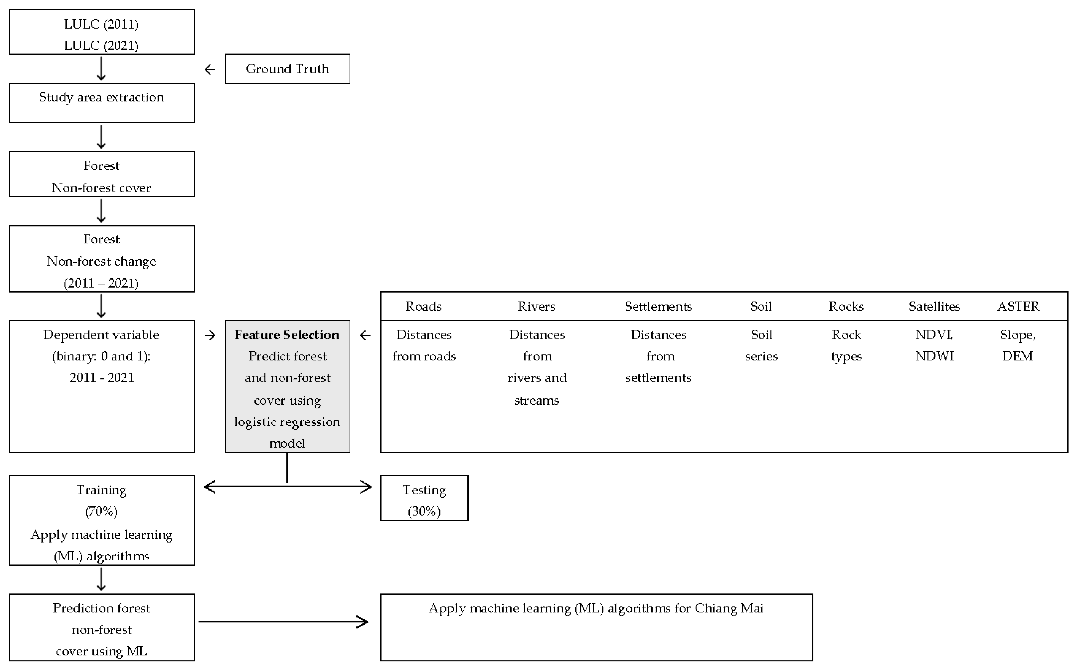
2. Materials and Methods

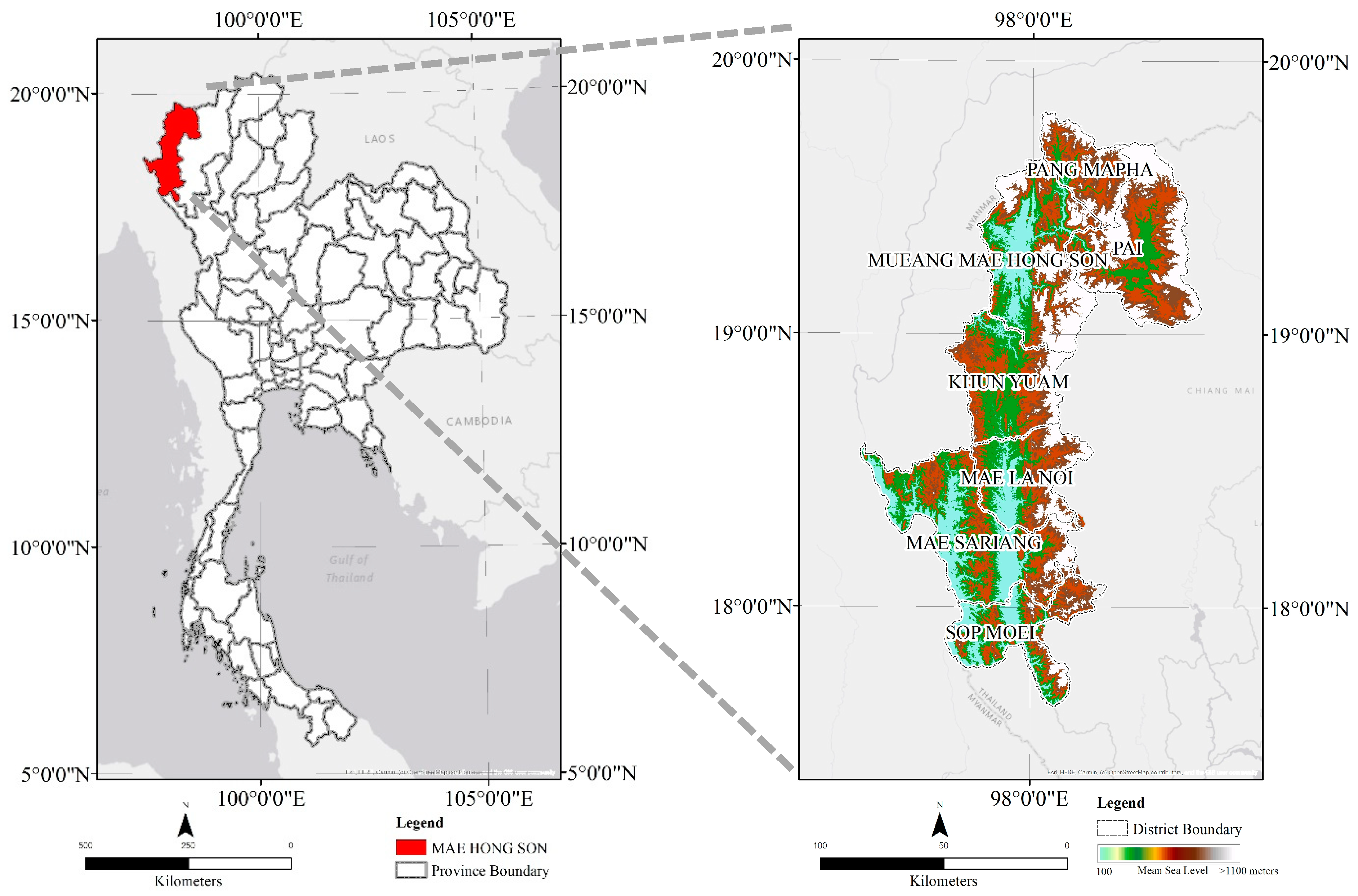
2.1. Study Area

Figure 1 shows the study area. Mae Hong Son Province, covering an area of 12,867 square kilometers, is predominantly characterized by complex high mountain ranges with abundant natural forests. The forest area in this province is approximately 10,619.93 square kilometers, accounting for 83.71% of the total provincial area. The topography of Mae Hong Son features parallel mountain ranges aligned in the north–south direction. The prominent mountain ranges include the Daen Lao Range, located in the northernmost part of the province and forming the border between Thailand and Myanmar, and the Thanon Thong Chai Range, which is further divided into three sub-ranges: the Western Thanon Thong Chai Range (forming the border with Myanmar), the Central Thanon Thong Chai Range (situated between the Yuam River and the Mae Chaem River), and the Eastern Thanon Thong Chai Range (serving as the boundary between Mae Hong Son and Chiang Mai). Mae Ya Peak, the highest point in Mae Hong Son, is in the Eastern Thanon Thong Chai Range in the northeastern part of Pai District. Mae Hong Son has an elevation of approximately 2005 m above sea level and limited arable land suitable for cultivation, covering only 1861.59 square kilometers, which is primarily located in Mae Sariang, Khun Yuam, and Pai Districts.

2.2. Change Detection Analysis

Detecting changes in forest areas is crucial for understanding past and present trends and making predictions for the future. This study focused on the period from 2011 to 2021 to assess the trends of change over the past decade. Figure 2 shows the forest cover during 2011 and 2021. Land cover comparisons were conducted sequentially for the study period. Given the large extent of the forest area, continuous changes over several years may not exhibit significant differences compared to highly urbanized areas where land use changes occur more frequently. The LULC data used in this study were provided by the country’s Land Development Department and underwent thorough accuracy assessments.

Table 1. Land use/land cover classification in study area.

Class Name	Sub-Class Name	2011 Land Area (sq km)	2021 Land Area (sq km)	Change Detection (sq km)
Non-forest	Waterbodies	40.30	52.76	12.46
	Agriculture	2249.47	1863.70	−385.76
	Built-up area	124.56	150.61	26.06
Forest	Forest	10,272.68	10,619.93	347.24
	Total	12,687.00	12,687.00

shows that the data layers were categorized into two main classes: non-forest and forest. The non-forest class included sub-classes such as urban, waterbodies, and vegetation, while all types of forests were classified under the forest class.

2.3. Forest Cover Change Variable

To establish the dependent variable, binary classification of forest cover change between 2011 and 2021 was performed. The resulting raster dataset was categorized into two distinct classes: “no change” (represented by the value 0), indicating areas where the forest remained intact, and “forest change” (represented by the value 1), signifying regions where the forest was converted to non-forest land cover types. To examine the relationship between the dependent and independent variables using a logistic regression model (LRM), sample points were randomly selected and divided into two categories: 500 points with forest changes and 500 points without forest changes. Subsequently, the data were split into two sets: a training set with 700 points for model creation and a testing set with 300 points for accuracy verification as shown in Figure 3.

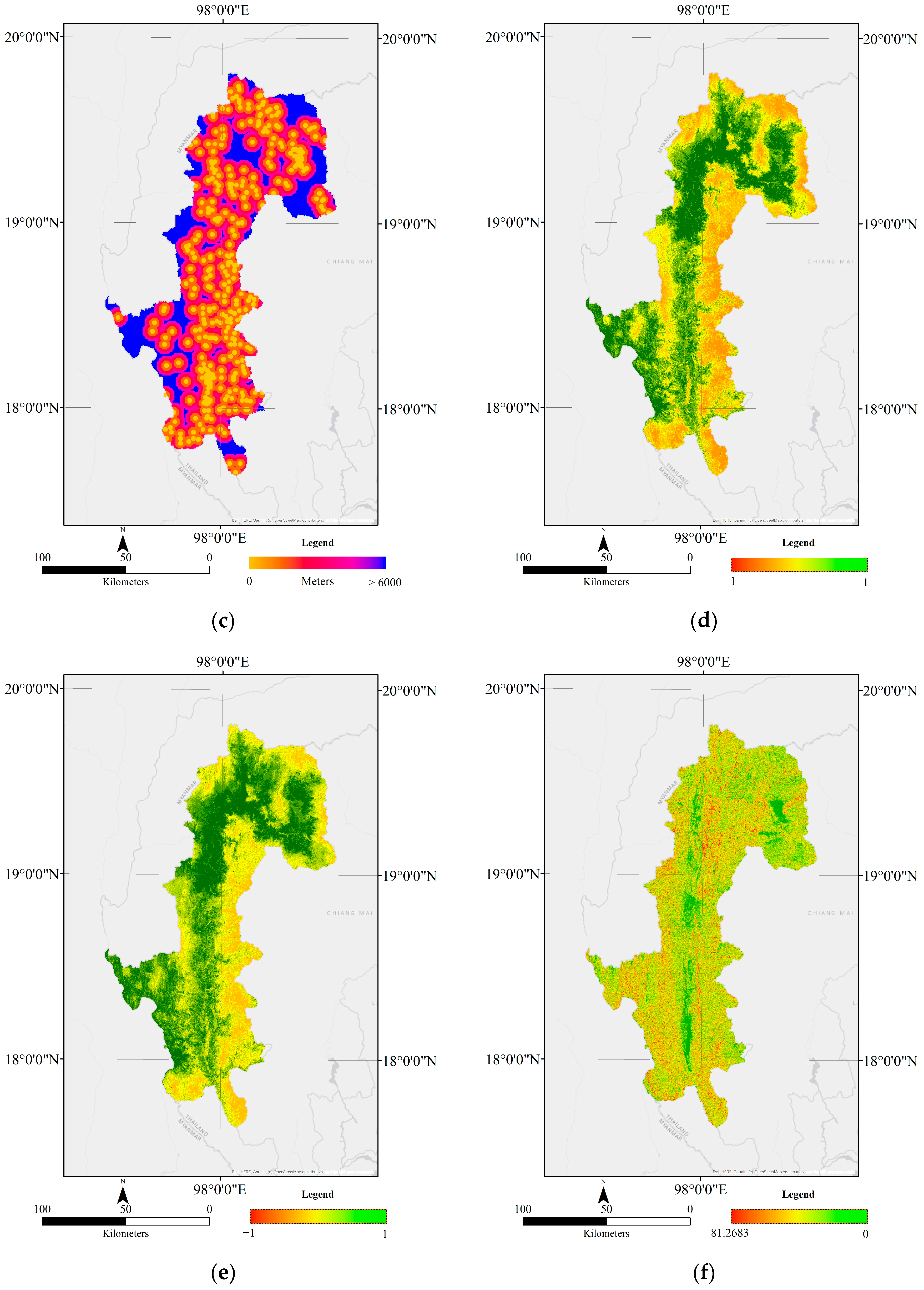
2.4. Explanatory Variables of Forest Cover Change

Figure 4 and

Table 2. Explanatory variables of forest cover change.

Variable	Original Data	Source
Forest change	Land use change	Google Earth Engine
Distances from roads, waterbodies, and settlements	Roads, waterbodies, and settlements	Land Development Department
Soil series and rock types	Soil series and rock types	Department of Environmental Quality Promotion
DEM	DEM	ASTER Global Digital Elevation Map
NDVI and NDWI	Landsat ETM+/OLI	Google Earth Engine

show the explanatory variables of forest cover change.

Table 3. The details of the class ranges for distances from roads, waterbodies, and settlements and slope.

Class Level	Distances from Roads (Meters)	Distances from Settlements (Meters)	Distances from Waterbodies (Meters)	DEM (Meters)	Slope (Degrees)
Level 1	0–400	0–1500	0–500	−33–420	0–10
Level 2	401–1000	1500–3000	501–1500	421–620	11–30
Level 3	1001–1500	3001–4500	1501–3000	621–820	31–40
Level 4	1501–2000	4500–6000	3000–4500	821–1020	41–50
Level 5	>2000	>6000	>4500	1021–2016	>50

shows that distances from settlements, roads, and waterbodies, as well as position classes, were taken into account as potential explanatory variables for forest cover change. Euclidean distances were calculated from settlements, roads, and waterbodies.

Topography exerts a certain degree of influence on forest cover change. Consequently, the classification of slope and the digital elevation model (DEM) position was considered essential for understanding the changes in forest cover. Table 3 provides details of the class ranges of the DEM and slope. The slope and DEM position classes were derived using ASTER GDEM and the topographic position index (TPI), as outlined by Weiss [26]. The NDVI and NDWI, which are indices that measure vegetation richness, were used as independent variables in this study. These indices used annual averages, and the data were obtained from Landsat ETM 7 and Landsat OLI 8 between 2011 and 2021 through the Google Earth Engine. The NDVI and NDWI are used to measure the richness of vegetation at a particular time, which influences changes in land cover types, such as forests.

Furthermore, rock types and soil series were also considered factors influencing forest cover change. The data for these variables were obtained from the Department of Environmental Quality Promotion between 2011 and 2021. The rock type and soil series data had different characteristics depending on their specific types.

Table 4. The details of the soil series.

Legend	Description
1	Lowland areas with gray clay soils (soil group numbers 5 and 7)
2	Lowland areas with gray loamy soils (soil group numbers 18, 59, and 59B)
3	Lowland areas with gray loamy riverbank soils (soil group number 21)
4	Upland areas with loamy soils found on both sides of riverbanks (soil group numbers 33, 38, and 38B)
5	Upland areas with clay soils and slopes (soil group numbers 29B, 29C, 29D, 29E, 30B, 30D, 30E, 31, 31B, 31C, 31D, and 31E)
6	Upland areas with loamy soils and slopes (soil group numbers 35, 35B, 35C, 36, 60, and 60B)
7	Upland areas with sandy soils (soil group numbers 44B and 44C)
8	Upland areas with moderately deep soils and slopes (soil group numbers 56B, 56C, 56D, and 56E)
9	Upland areas with shallow soils and slopes (soil group numbers 48B, 48C, 48D, 48E, and 49B)
10	Upland areas with shallow bedrock and slopes (soil group number 47D)
11	Upland areas with extremely steep slopes or mountainous areas (soil group number 62). These areas were not studied, surveyed, or classified based on their soil characteristics and properties because they have slopes greater than 35%. They are considered difficult to manage and maintain for agriculture and consist of very shallow to deep soils, and they potentially contain boulders, rock fragments, and exposed bedrock scattered on the soil surface.

shows the details of the soil series, and

Table 5. The details of the rock types.

Legend	Description
Qa	Alluvial deposits: sandy clay, clayey sand, lateritic soil, and clay
Qt	Terrace deposits: gravel, sand, and laterite
Qc	Calluvial and residual deposits
T	Claystone, siltstone, sandstone, mudstone, diatomite, and lignite
J	Red conglomerate and reddish-brown sandstone intercalated with shale and mudstone
Ju	Sandstone, siltstone, conglomerate, limestone, bivalve, and ammonite
TRJ	Greenish-gray sandstone, reddish-brown siltstone, limestone, and conglomerate
TR2	Shale, chert, and thin-bedded limestone with bivalve fossils
TR1	Red conglomerate, sandstone, and red to reddish-brown shale
PTR	Shale, siltstone, and dark gray to greenish-gray sandstone intercalated with thin-bedded chert
Pph	Gray limestone with thick-bedded, distinct karst topography and shale
Pkl	Sandstone, chert, and gray shale
P	Sandstone, gray siltstone, red shale, mudstone, and gray thick-bedded limestone
CP	Sandstone, shale, red conglomerate, chert, and slaty shale
C2	Shale, siltstone, and gray sandstone interbedded with chert
C1	Gray sandstone, gray shale, green-to-gray chert, and limestone interbedded with shale
C	Sandstone interbedded with gray shale, conglomerate, shale, chert, limestone, and mudstone
D	Shale interbedded with limestone and sandstone
SDC	Gray shale interbedded with limestone, with fossils of nautiloids, gastropods, and conodonts
SD	Sandstone interbedded with siltstone, shale, limestone, and phyllitic shale, with tentaculite fossils
O	Gray argillaceous limestone interbedded with mudstone and shale, with fossils of conodonts and nautiloids
EO	White banded marble and quartz–mica schist
E	Quartzite and sandstone interbedded with shale and slaty shale
bs	Volcanic rock: basalt, black, and gray
TRgr	Igneous rock: biotite granite, hornblende–biotite granite, muscovite granite with equigranular-to-porphyritic texture, and fine-grained leucogranite
TRm	Migmatite, unclassified granite, gneiss, schist, quartzite, and sandstone
Cgr	Igneous rock: granite in contact metamorphism zone, cataclastic granite, and biotite granite

shows the details of the rock types.

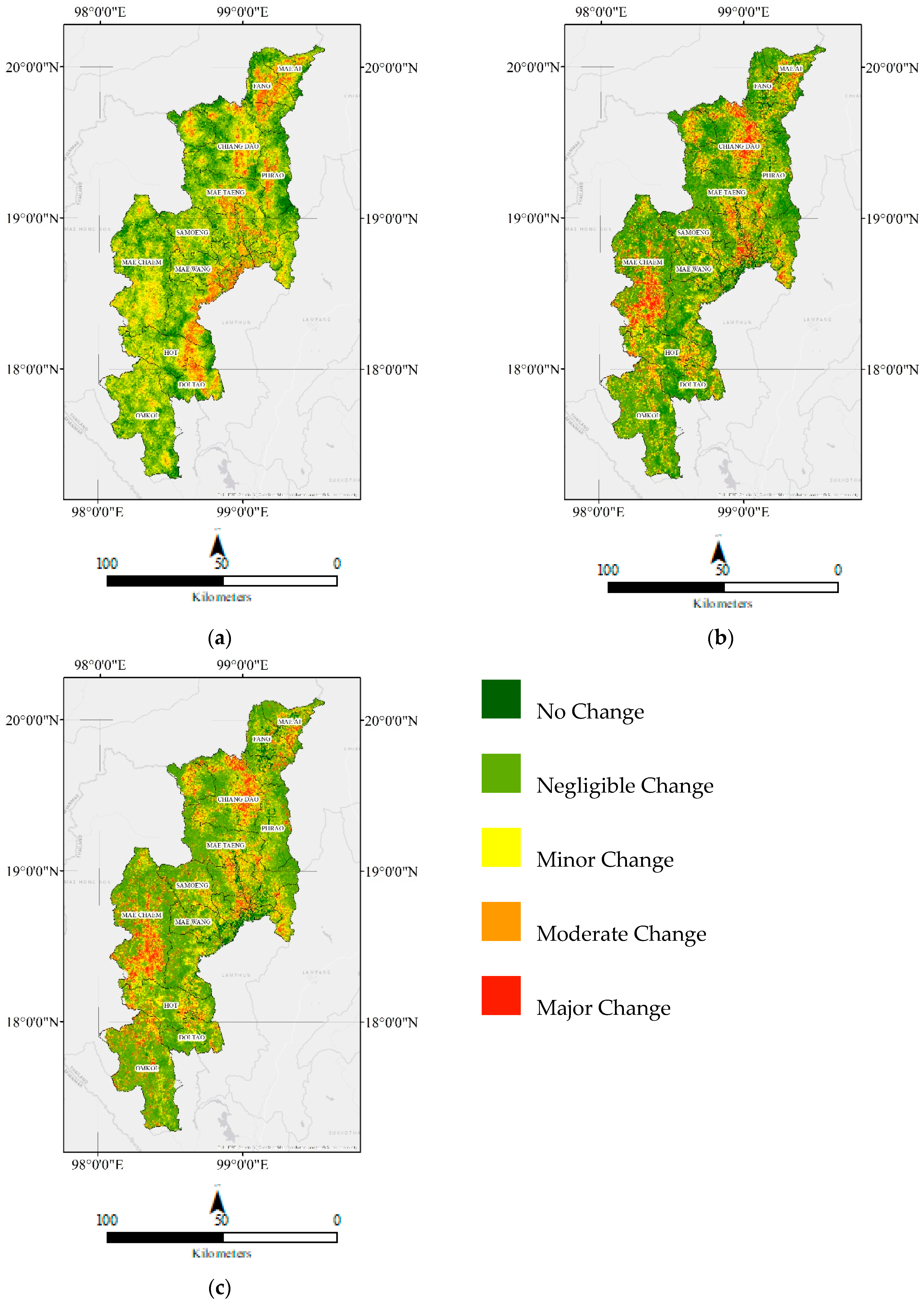
2.5. Model Calibration and Classification of Forest Cover Change

2.5.1. Logistic Regression Model (LRM)

To analyze and model the forest change from 2011 to 2021, an LRM was employed using RStudio-4.3.1. This study aimed to assess the impact of explanatory variables on forest cover change during this period and predict the probability of change by 2021. The dependent variable for the 2011–2021 period was binary, indicating the presence (1) or absence (0) of forest change. In the logistic function, the probability of forest change (p) was considered a function of the explanatory variables and was defined as follows:

$$p=E\left(\mathrm{Y}\right)\frac{e^{{\beta }_0+{\beta }_1{X}_1+{\beta }_2{X}_2+{\beta }_3{X}_3+{\beta }_4{X}_4}}{1+e^{{\beta }_0+{\beta }_1{X}_1+{\beta }_2{X}_2+{\beta }_3{X}_3+{\beta }_4{X}_4}}$$

(1)

where E(Y) is the expected value of the dependent variable (Y), ${\beta }_0$ is a constant to be estimated, and ${\beta }_i$ is a coefficient to be estimated for each explanatory variable ($X_1$). This logistic function (Equation (1)) can be transformed into a linear function (Equation (3)), known as the logit or logistic transformation, as shown in Equation (2):

$${logit}_p={logit}_e\left(\frac{p}{1-p}\right)$$

(2)

$${logit}_p={\beta }_0+{\beta }_1{X}_1+{\beta }_2{X}_2+{\beta }_3{X}_3+{\beta }_4{X}_4$$

(3)

To ensure that the data were suitable for modeling, a normalization process was applied to all independent variables, scaling them to a range between 0.1 and 0.9. Subsequently, the LRM underwent a calibration phase, where the explanatory variables corresponding to the year 2000 were incorporated as independent variables. A stepwise selection approach was employed to systematically evaluate eight predictor sets and consequently select the best among them.

Following the approach used by van Gils et al. [27], the Akaike information criterion (AIC) index was used to determine the model that fit best with the fewest predictors.

The regression equation for the most accurate predictor set was then used to calculate the probability of forest cover change in 2011. This probability was subsequently utilized to predict forest change from 2011 to 2021.

After identifying the factors associated with forest change, some were selected for further testing with the RF and SVM machine learning algorithms.

2.5.2. Random Forest (RF)

The random forest classifier is composed of numerous decision tree classifiers, each of which is constructed using a randomly sampled subset of features from the input vector. Each classifier casts a vote for the most likely class, and the input vector is categorized into the class receiving the highest number of votes across all classifiers [28]. The implementation of the random forest classifier in this study involved growing each tree by randomly selecting features or combinations of features at each node. For each feature (combination) selected, the bagging technique was employed, and a training dataset was generated by randomly drawing instances with replacements from the original training set. To classify a new input vector, the class with the most cumulative votes from all the tree predictors in the forest was chosen. The decision tree construction process required the selection of an attribute selection measure and a pruning technique.

Among the various approaches to attribute selection, the Information Gain Ratio and the Gini index are the most utilized metrics.

The random forest classifier employed the Gini index as its attribute selection metric, quantifying the impurity of an attribute for the classes. For a given training set (T), the Gini index is defined as follows:

$$\mathsf{\Sigma }{\sum }_{j\ne i} \left(f\left(C_i,T\right)/\left|T\right|\right)\left(f\left(C_j,T\right)/\left|T\right|\right)$$

(4)

where f(C_i, T)/|T| represents the probability that a randomly chosen instance belongs to class C_i.

In the random forest classifier, each decision tree was grown to its maximum depth utilizing a combination of features on new training data. Notably, these fully grown trees remained unpruned, which is a significant advantage of the random forest approach over other decision tree methods that employ pruning strategies.

Findings have indicated that the pruning techniques used have a significant impact on the performance of tree-based classifiers [29].

2.5.3. Support Vector Machine (SVM)

An SVM is a supervised machine learning algorithm originally proposed by Vapnik et al. [30]. It is a classification technique that maps non-linear input data into a higher-dimensional feature space, where the data become linearly separable through the construction of a hyperplane. The kernel function is the mathematical function employed for this data transformation. Using a training dataset, an SVM maps original input vectors into a high-dimensional feature space. In this transformed space of n dimensions, a separating hyperplane is determined, which partitions the data points of different classes. An SVM identifies the hyperplane that maximizes the margin between the classes. Any data point lying on one side of this hyperplane is assigned to the +1 class, while points on the other side are assigned to the −1 class. The properties of new, unseen data points can then be used to predict which of the two classes they belong to. The support vectors are the training data points closest to the separating hyperplane. Once this decision boundary is found, it can be used to classify future data instances. The separating hyperplane for linearly separable data in an original vector space can be represented using Equation (5):

$$wx+b=0$$

(5)

Vector w, which is normal to the hyperplane, and constant b are learned from a training set of linearly separable instances. SVMs are formulated to solve a constrained quadratic optimization problem (Equation (6)), ensuring that the SVM solution is always globally optimal.

$${\mathrm{m}\mathrm{i}\mathrm{n}}_{\omega } \frac{1}{2}\parallel \omega {\parallel }^2+C{\sum }_i {\xi }_i$$

(6)

This equation is subject to the following constraints:

$$y_i\left(x_{i}w+b\right)⩾1-{\xi }_i{\xi }_i⩾0,\forall i$$

(7)

For linearly inseparable data in an original input space, an SVM employs kernel functions to implicitly map the data into a higher-dimensional feature space where the classes become linearly separable [31]. This non-linear mapping allows the SVM to construct the separating hyperplane in the new high-dimensional space without explicitly computing the mappings or increasing the computational complexity of solving the quadratic programming problem. The kernel function provides a way to calculate the similarities between vectors in the high-dimensional space for a linearly inseparable case by instead computing these similarities using the original lower-dimensional input vectors.

2.6. Measuring and Verifying Classification Accuracy

For this study, a confusion matrix was utilized to inspect and evaluate the accuracy of the prediction results. Consequently, the predictions were categorized into four types as shown in the

Table 6. Details of the confusion matrix.

Actual class		Predicted class
		No change	Change
	No change	True Positive (TP)	False Positive (FP)	$\mathrm{Positive} \mathrm{prediction} \mathrm{value}=\frac{\mathrm{TP}}{\mathrm{TP}+\mathrm{FP}}$
	Change	False Negative (FN)	True Negative (TN)	$\mathrm{Negative} \mathrm{prediction} \mathrm{value}=\frac{\mathrm{TN}}{\mathrm{TN}+\mathrm{FN}}$
		$\mathrm{Sensitivity}=\frac{\mathrm{TP}}{\mathrm{TP}+\mathrm{FN}}$	$\mathrm{Specificity}=\frac{\mathrm{TN}}{\mathrm{TN}+\mathrm{FP}}$	$\mathrm{Accuracy}=\frac{\mathrm{TP}+\mathrm{TN}}{\mathrm{TP}+\mathrm{FN}+\mathrm{FP}+\mathrm{TN}}$

:

• True Positive (TP): the model predicts change, and the ground truth is change.
• True Negative (TN): the model predicts no change, and the ground truth is no change.
• False Positive (FP): the model predicts change, but the ground truth is no change.
• False Negative (FN): the model predicts no change, but the ground truth is change.

After obtaining the TP, FP, FN, and TN values, the p-value and kappa coefficient index were verified.

The p-value was utilized to evaluate the significance of the results compared to the null hypothesis during the statistical testing procedures. A null hypothesis states that there is no relationship or connection between the two variables being investigated. Essentially, one variable does not impact or influence the other in any way. Conversely, an alternative hypothesis claims that the independent variable exerts an influence over the dependent variable and that the results are important for corroborating or providing supporting evidence for the theory currently under investigation. A p-value less than 0.05 (with 0.05 typically being the standard threshold) is characterized as indicating statistical significance. When the p-value falls below 0.05, it demonstrates substantial evidence against the null hypothesis, as the likelihood of the null hypothesis being true is computed to be less than 5%. Consequently, due to this low probability, the null hypothesis is rejected, and, instead, the alternative hypothesis is accepted as the more plausible scenario.

Cohen’s kappa coefficient is a statistical measure that is frequently employed to evaluate reliability. In this context, it can be utilized to assess the reliability between the training and testing phases. The kappa coefficient reflects and quantifies the degree of agreement between the frequencies of two distinct sets of data, with one set obtained during the training phase and the other obtained during the testing phase. There is an established scale for interpreting the values of the kappa coefficient [32], as outlined below see the

Table 7. The scale for kappa value interpretation.

Kappa	Interpretation
<0%	No agreement
0.01%–20%	Slight agreement
21%–40%	Fair agreement
41%–60%	Moderate agreement
61%–80%	Substantial agreement
81%–100%	Perfect agreement

.

Having successfully verified the accuracy of the linear regression, RF, and SVM models, the subsequent step involved conducting further experiments utilizing these models along with the previously selected factors, as well as all eight factors, in the areas of Chiang Mai and Phetchabun Provinces. This research endeavored to determine whether these models and factors could yield accurate results when applied to different study areas.

Chiang Mai was selected due to its forested areas being adjacent to Mae Hong Son. This experiment aimed to assess whether these factors and models could accurately predict outcomes in high-altitude areas, and this was intended to expand the scope of knowledge regarding the reliability of these models across diverse areas by providing more definitive insights.

Following the determination of the model’s accuracy, the FRs were normalized to the interval of probability values [0, 1] in the form of Relative Frequency (RF). The RF was computed for each class by utilizing Equation (8):

$$RF=\frac{{FR}_{ij}}{{\sum }_{i=1}^m{FR}_{ij}}$$

(8)

Equation (9) was utilized to compute the Prediction Rate (PR) for the evaluation of each conditional factor in the training dataset after normalization:

$$PR=\frac{{(RF}_{max}-{RF}_{min})}{{{(RF}_{max}-{RF}_{min})}_{min}}$$

(9)

In conclusion, the forest susceptibility index (FSI) was computed by adding the products of the PR for each factor and the RF for each class, as illustrated below:

$$FSI=\sum (PR\ast RF)$$

(10)

A forest susceptibility map was produced using the FSI values and the entire conceptual framework of the research, as depicted in Figure 5.

3. Results

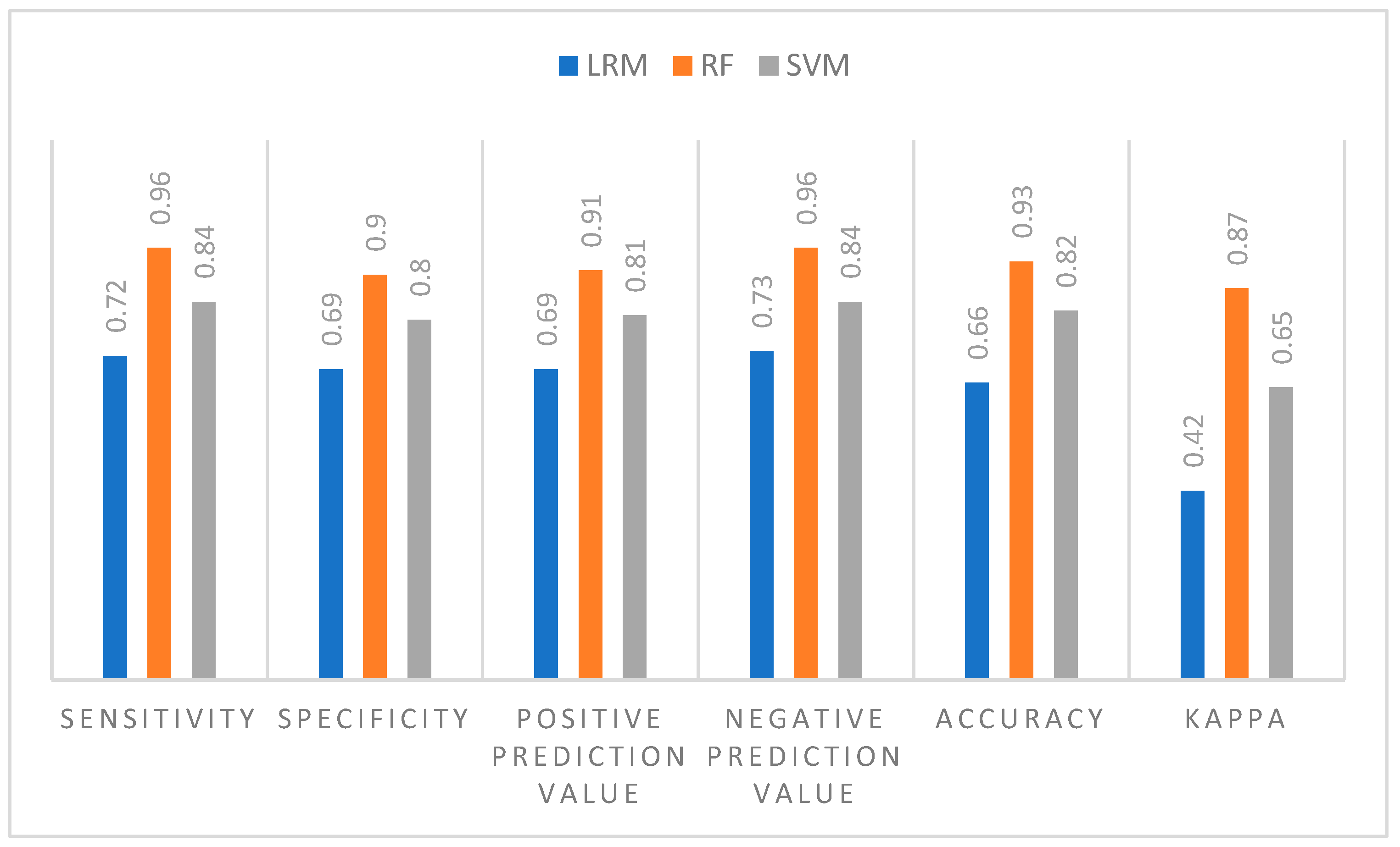
3.1. Measuring and Verifying Classification Accuracy

The study of factors influencing forest cover change in Mae Hong Son identified six relevant factors: soil series, rock types, slope, the NDVI, the NDWI, and the distances to settlement areas. These factors were utilized to construct a binary logistic regression model to investigate the relationship between the factors and forest cover changes in the province.

Table 8. Relationships between dependent variable and independent variables.

Coefficients
	Estimate	Std. Error	z Value	Pr(>|z|)	Significance
Intercept	6.263955	0.678038	9.238	<2 × 10−16	***
Soil series	−0.374430	0.079131	−4.732	2.23 × 10−6	***
Rock types	−0.016687	0.005221	−3.196	0.00139	**
DEM	−0.013484	0.041603	−0.324	0.74585
Slope	−0.356960	0.058326	−6.120	9.35 × 10−10	***
NDVI	−0.831213	0.109684	−7.578	3.50 × 10−14	***
NDWI	1.045128	0.106785	9.787	<2 × 10−16	***
Distances from roads	−0.039336	0.039755	−0.989	0.32243
Distances from waterbodies	0.051698	0.037715	1.371	0.17045
Distances from settlements	−0.533503	0.035352	−15.091	<2 × 10−16	***

The significance levels are denoted as *** for p ≤ 0.001 and ** for 0.001 < p ≤ 0.01.

shows the relationships between the dependent variable and the independent variables.

The Akaike information criterion (AIC) was 3261.8, and there were four Fisher Scoring iterations.

The estimates show the y-intercept value and the coefficient associated with each predictor variable.

Std. Error indicates the standard error of the coefficient estimates, representing the accuracy of the coefficients. The larger the standard error, the less confidence we have in an estimate.

The z-values refer to the coefficient estimates divided by their standard errors.

Pr(>|z|) is the p-value corresponding to the z-statistic. The smaller the p-value, the more significant the estimate.

The Akaike information criterion (AIC) provides scores that measure the relative qualities of competing models.

Fisher Scoring provides information about the iterations of a model. Many iterations may indicate concern that an algorithm is not converging properly.

The results of the binary logistic regression analysis could be written as a multiple linear equation before creating a probability map of forest area change, as shown in Equation (11):

         Probability of forest cover change = 6.263955 + (−0.374430 ∗ “Soil Series”) +
        (−0.016687 ∗ “Rock Types”) + (−0.356960 ∗ “Slope”) + (−0.831213 ∗ “NDVI”) +
 (1.045128 ∗ “NDWI”) + (−0.533503 ∗ Distance to Settlement)

(11)

3.2. Verifying Variables Influencing Forest Cover Change in Mae Hong Son

The model was subsequently used to predict forest cover changes in Mae Hong Son using the binary error matrix to assess the prediction accuracy of the logistic regression model.

The results showed that the sensitivity was 0.72, and the specificity was 0.69. Furthermore, the negative prediction value was 0.73, and the positive prediction value was 0.69. The overall accuracy of the constructed model was 0.71, which fell within the substantial level and was considered reliable (

Table 9. The accuracy of forest cover change occurrence using the binary error matrix for the logistic regression model.

Ground truth		Model prediction
		No change	Change
	No change	417	190	$0.69$
	Change	161	425	$0.73$
		$0.72$	$0.69$	$0.65$

Overall accuracy: 0.65. Kappa coefficient: 0.42.

).

The variables identified from the LRM, namely, soil series, rock types, slope, the NDVI, the NDWI, and distances to settlement areas, were employed to construct machine learning (ML) models utilizing two algorithms: RF and SVM. The purpose was to evaluate whether the RF and SVM models exhibited superior performance to the LRM.

The accuracy of the forest cover change predictions for Mae Hong Son was evaluated using the binary error matrix for the RF model. The results showed that the sensitivity was 0.96, and the specificity was 0.90. Furthermore, the negative prediction value was 0.96, and the positive prediction value was 0.91. The overall accuracy of the constructed model was 0.93, which fell within the perfect level and was considered extremely reliable (

Table 10. The accuracy of forest cover change occurrence using the binary error matrix for the random forest model.

Ground truth		Model prediction
		No change	Change
	No change	575	59	$0.91$
	Change	21	538	$0.96$
		$0.96$	$0.90$	$0.93$

Overall accuracy: 0.93. Kappa coefficient: 0.87.

).

The accuracy of the forest cover change predictions for Mae Hong Son was evaluated using the binary error matrix for the SVM model. The results showed that the sensitivity was 0.84, and the specificity was 0.80. Furthermore, the negative prediction value was 0.84, and the positive prediction value was 0.81. The overall accuracy of the constructed model was 0.82, which fell within the substantial level and was considered reliable (

Table 11. The accuracy of forest cover change occurrence using the binary error matrix for the support vector machine model.

Ground truth		Model prediction
		No change	Change
	No change	503	117	$0.82$
	Change	93	480	$0.84$
		$0.84$	$0.80$	$0.82$

Overall accuracy: 0.82. Kappa coefficient: 0.65.

).

Figure 6 compares the accuracy across all models. It is evident that both machine learning algorithms (RF and SVM) yielded superior values for sensitivity, specificity, positive prediction, negative prediction, accuracy, and the kappa coefficient compared to the LRM. However, the RF model outperformed the SVM across all evaluation metrics. Figure 7 shows the classifications of all models.

3.3. Verifying Variables Influencing Forest Cover Change in Chiang Mai

The soil series, rock types, slope, NDVI, NDWI, and distances from settlements were the six significant characteristics that were shown to be associated with the change in forest cover in Mae Hong Son. Using these variables, a logistic regression model, a support vector machine, and a random forest were built, and the models were verified for Chiang Mai.

Figure 8 compares the accuracy values of all models in the case of Chiang Mai Province. After analyzing the performances of all models, it was clear that both machine learning algorithms (RF and SVM) outperformed the LRM in terms of sensitivity, specificity, positive prediction, negative prediction, accuracy, and the kappa coefficient, as was the case in Mae Hong Son. Specifically, the RF model beat the SVM on all assessment measures. Figure 9 shows the classifications of all models for Chiang Mai.

4. Discussion

Naturally, understanding the underlying causes of forest cover change necessitates examining the factors influencing variations in forest cover. In remote mountainous areas like the Mae Hong Son and Chiang Mai Provinces in Thailand, research on the specific factors driving changes in forest area is still scarce.

A list of important variables from previous studies is provided in

Table 12. A list of important variables from previous studies.

Authors	Variables	Period	Techniques	Results
Kumar et al. [33]	Distances from forest edges, roads, and settlements and slope position classes as explanatory variables of forest change	1990 to 2010	LRM	The LRM successfully predicted the forest cover in 2010 with reasonably high accuracy (ROC = 87%).
Nurda et al. [34]	Distances from rivers, distances from roads, elevation, LULC, and settlements	2003 to 2018	AHP	In the AHP method, the influential criteria had higher weights and were ranked as follows: settlements, elevation, distances from roads, and distances from rivers.
Guo et al. [35]	Land use; night light; settlement density; GDP; state, county, and township roads; lithological data; precipitation; evaporation; and DEM	1980 to 2018	Generalized linear model (GLM) regression	The effects of population and gross domestic product (GDP) on the forest changes weakened, and the influence of land use change markedly increased.

[33,34,35]. This study discovered that the distance from a road also affects the shift in forest cover.

The findings show that areas of forest change in Northern Thailand are more common on low slopes and near roads due to their vulnerability to destruction. People need land to build housing and farms. This is in line with the results of studies conducted in several countries, including Cameroon [36], Indonesia [37], and Mexico [38]. People destroy rock layers and soil that are suitable for agriculture. In addition, the portion of the NDVI related to forest area change is between 0.3 and 0.6, which does not indicate an area of healthy vegetation. We can assume that this is agricultural land.

Researchers discovered that changes in forest areas are significantly influenced by humans. However, in this study, changes in forest cover were impacted by the NDVI, the NDWI, rock types, and soil series.

Various variables might affect forest cover change, including locations, cultures, and economic situations. As a result, the goal of this research was to obtain a thorough understanding of the factors that influence the changes in forest areas in these regions. It is anticipated that the results will be widely embraced, will assist in the creation of practical plans for restoring ecosystems, and will encourage long-term sustainable land use management. According to this study, machine learning (ML) contributes significantly to our understanding of the factors influencing change in forest areas. In the future, the use of deep learning is another option for studying the factors affecting change. Some researchers have already performed experiments using this technology [10].

5. Conclusions

This study’s findings indicate that factors such as the soil, rock type, NDVI, NDWI, slopes, and urban distance influence changes in forest areas in the northern portions of the country. Furthermore, our objective was to examine whether machine learning methods can classify forest changes with higher precision compared to logistic regression models. We found that both the RF and SVM machine learning algorithms demonstrated higher values for the kappa coefficient, sensitivity, specificity, and accuracy. We evaluated both positive and negative predictions, specifically concentrating on the random forest (RF) algorithm’s sensitivity. Additionally, our goal was to assess these variables’ potential for reclassification. We found that both the Mae Hong Son factors and the RF and SVM algorithms can be applied in Chiang Mai.

This study’s outcomes were more accurate when a machine learning system was used. Furthermore, machine learning was able to correctly separate the data by fine-tuning the parameters to obtain the right value via experimentation.

We discovered that the machine learning techniques produced precise prediction results in our investigation. The method used in this study has the following benefits: (1) it can categorize changes in forest cover; (2) it identifies the factors that influence these changes; (3) it is a useful tool to support decision-making; and (4) it may enhance future predictions of changes in forest cover at a macro-level.

One of this study’s limitations is that the local government of Thailand provides data on changes in forest cover in a static manner, and they have to be updated on a regular basis. Future research should be useful if the Thai local government utilizes an API and posts the data online.

This research validates the ability of machine learning to provide more precise findings related to forest changes. Future research, machine learning, and APIs might be used to generate additional knowledge in other scientific domains. The locations of forest fires, landslides, and forest floods may all be predicted in the future using these kinds of data and methods.

References

1. Putz, F.E.; Blate, G.M.; Redford, K.H.; Fimbel, R.; Robinson, J. Tropical forest management and conservation of biodiversity: An overview. Conserv. Biol. 2001, 15, 7–20. [Google Scholar] [CrossRef]
2. Mitchard, E.T. The tropical forest carbon cycle and climate change. Nature 2018, 559, 527–534. [Google Scholar] [CrossRef] [PubMed]
3. FAO; UNEP. The State of the World’s Forests 2020: Forests, Biodiversity and People; FAO: Rome, Italy, 2020. [Google Scholar]
4. Mitchell, A.L.; Rosenqvist, A.; Mora, B. Current remote sensing approaches to monitoring forest degradation in support of countries measurement, reporting and verification (MRV) systems for REDD+. Carbon Balance Manag. 2017, 12, 9. [Google Scholar] [CrossRef] [PubMed]
5. Crutzen, P.J. The “anthropocene”. In Earth System Science in the Anthropocene; Springer: Berlin/Heidelberg, Germany, 2006; pp. 13–18. [Google Scholar]
6. FAO. The State of the World’s Forests 2018—Forest Pathways to Sustainable Development; FAO: Rome, Italy, 2018. [Google Scholar]
7. Díaz, S.; Settele, J.; Brondízio, E.; Ngo, H.; Guèze, M.; Agard, J.; Zayas, C. Summary for Policymakers of the Global Assessment Report on Biodiversity and Ecosystem Services of the Intergovernmental Science-Policy Platform on Biodiversity and Ecosystem Services; Intergovernmental Science-Policy Platform on Biodiversity and Ecosystem Services: Bonn, Germany, 2019. [Google Scholar]
8. UN. The Sustainable Development Goals Report; United Nations: New York, NY, USA, 2016. [Google Scholar]
9. Dibs, H.; Ali, A.H.; Al-Ansari, N.; Abed, S.A. Fusion Landsat-8 Thermal TIRS and OLI Datasets for Superior Monitoring and Change Detection using Remote Sensing. Emerg. Sci. J. 2023, 7, 428–444. [Google Scholar] [CrossRef]
10. Mirpulatov, I.; Illarionova, S.; Shadrin, D.; Burnaev, E. Pseudo-Labeling Approach for Land Cover Classification Through Remote Sensing Observations With Noisy Labels. IEEE Access 2023, 11, 82570–82583. [Google Scholar] [CrossRef]
11. Praticò, S.; Solano, F.; Di Fazio, S.; Modica, G. Machine Learning Classification of Mediterranean Forest Habitats in Google Earth Engine Based on Seasonal Sentinel-2 Time-Series and Input Image Composition Optimisation. Remote Sens. 2021, 13, 586. [Google Scholar] [CrossRef]
12. Brovelli, M.A.; Sun, Y.; Yordanov, V. Monitoring Forest Change in the Amazon Using Multi-Temporal Remote Sensing Data and Machine Learning Classification on Google Earth Engine. ISPRS Int. J. Geo-Inf. 2020, 9, 580. [Google Scholar] [CrossRef]
13. Li, Y.; Li, M.; Li, C.; Liu, Z. Forest aboveground biomass estimation using Landsat 8 and Sentinel-1A data with machine learning algorithms. Sci. Rep. 2020, 10, 9952. [Google Scholar] [CrossRef] [PubMed]
14. Hansen, M.C.; Potapov, P.V.; Moore, R.; Hancher, M.; Turubanova, S.A.; Tyukavina, A.; Thau, D.; Stehman, S.V.; Goetz, S.J.; Loveland, T.R. High-resolution global maps of 21st-century forest cover change. Science 2013, 342, 850–853. [Google Scholar] [CrossRef]
15. Shimada, M.; Itoh, T.; Motooka, T.; Watanabe, M.; Shiraishi, T.; Thapa, R.; Lucas, R. New global forest/non-forest maps from ALOS PALSAR data (2007–2010). Remote Sens. Environ. 2014, 155, 13–31. [Google Scholar] [CrossRef]
16. Santoro, M.; Cartus, O.; Carvalhais, N.; Rozendaal, D.M.A.; Avitabile, V.; Araza, A.; de Bruin, S.; Herold, M.; Quegan, S.; Rodríguez-Veiga, P.; et al. The global forest above-ground biomass pool for 2010 estimated from high-resolution satellite observations. Earth Syst. Sci. Data 2021, 13, 3927–3950. [Google Scholar] [CrossRef]
17. Brink, A.B.; Eva, H.D. Monitoring 25 years of land cover change dynamics in Africa: A sample based remote sensing approach. Appl. Geogr. 2009, 29, 501–512. [Google Scholar] [CrossRef]
18. Petit, C.C.; Lambin, E.F. Integration of multi-source remote sensing data for land cover change detection. Int. J. Geogr. Inf. Sci. 2010, 15, 785–803. [Google Scholar] [CrossRef]
19. Nomura, K.; Mitchard, E. More Than Meets the Eye: Using Sentinel-2 to Map Small Plantations in Complex Forest Landscapes. Remote Sens. 2018, 10, 1693. [Google Scholar] [CrossRef]
20. Surono, S.; Afitian, M.Y.F.; Setyawan, A.; Eni Arofah, D.K.; Thobirin, A. Comparison of CNN Classification Model using Machine Learning with Bayesian Optimizer. HighTech Innov. J. 2023, 4, 531–542. [Google Scholar] [CrossRef]
21. Wang, L.; Ye, C.; Chen, F.; Wang, N.; Li, C.; Zhang, H.; Wang, Y.; Yu, B. CG-CFPANet: A multi-task network for built-up area extraction from SDGSAT-1 and Sentinel-2 remote sensing images. Int. J. Digit. Earth 2024, 17. [Google Scholar] [CrossRef]
22. Vega Isuhuaylas, L.; Hirata, Y.; Ventura Santos, L.; Serrudo Torobeo, N. Natural Forest Mapping in the Andes (Peru): A Comparison of the Performance of Machine-Learning Algorithms. Remote Sens. 2018, 10, 782. [Google Scholar] [CrossRef]
23. Potić, I.; Srdić, Z.; Vakanjac, B.; Bakrač, S.; Đorđević, D.; Banković, R.; Jovanović, J.M. Improving Forest Detection Using Machine Learning and Remote Sensing: A Case Study in Southeastern Serbia. Appl. Sci. 2023, 13, 8289. [Google Scholar] [CrossRef]
24. Siles, N.S. Spatial Modelling and Prediction of Tropical Forest Conversion in the Isiboro Sécure National Park and Indigenous Territory TIPNIS, Bolivia. Master’s Thesis, ITC: Faculty of Geo-information Science and Earth Observation, Enschede, The Netherlands, 2009. [Google Scholar]
25. Saleh, A. Modeling spatial pattern of deforestation using GIS and logistic regression: A case study of northern Ilam forests, Ilam province, Iran. Afr. J. Biotechnol. 2011, 10, 16236–16249. [Google Scholar] [CrossRef]
26. Weiss, A. Topographic position and landforms analysis. In Proceedings of the Poster Presentation, ESRI User Conference, San Diego, CA, USA, 9–13 July 2001. [Google Scholar]
27. van Gils, H.A.M.J.; Ugon, A.V.L.A. What Drives Conversion of Tropical Forest in Carrasco Province, Bolivia? AMBIO J. Hum. Environ. 2006, 35, 81–85. [Google Scholar] [CrossRef]
28. Breiman, L. Random Forests. Mach. Learn. 2001, 45, 5–32. [Google Scholar] [CrossRef]
29. Pal, M.; Mather, P.M. An assessment of the effectiveness of decision tree methods for land cover classification. Remote Sens. Environ. 2003, 86, 554–565. [Google Scholar] [CrossRef]
30. Vapnik, V.; Golowich, S.E.; Smola, A. Support vector method for function approximation, regression estimation and signal processing. In Proceedings of the 9th International Conference on Neural Information Processing Systems, Denver, CO, USA, 2–5 December 1996; pp. 281–287. [Google Scholar]
31. Aizerman, M.A.; Braverman, E.M.; Rozonoer, L.I. Theoretical foundation of potential functions method in pattern recognition. Avtomatika i Telemekhanika 2019, 25, 917–936. [Google Scholar]
32. Nichols, T.R.; Wisner, P.M.; Cripe, G.; Gulabchand, L. Putting the Kappa Statistic to Use. Qual. Assur. J. 2011, 13, 57–61. [Google Scholar] [CrossRef]
33. Kumar, R.; Nandy, S.; Agarwal, R.; Kushwaha, S.P.S. Forest cover dynamics analysis and prediction modeling using logistic regression model. Ecol. Indic. 2014, 45, 444–455. [Google Scholar] [CrossRef]
34. Nurda, N.; Noguchi, R.; Ahamed, T. Change Detection and Land Suitability Analysis for Extension of Potential Forest Areas in Indonesia Using Satellite Remote Sensing and GIS. Forests 2020, 11, 398. [Google Scholar] [CrossRef]
35. Guo, X.; Chen, R.; Meadows, M.E.; Li, Q.; Xia, Z.; Pan, Z. Factors Influencing Four Decades of Forest Change in Guizhou Province, China. Land 2023, 12, 1004. [Google Scholar] [CrossRef]
36. Mertens, B.; Lambin, E.F. Spatial modelling of deforestation in southern Cameroon. Appl. Geogr. 1997, 17, 143–162. [Google Scholar] [CrossRef]
37. Linkie, M.; Smith, R.J.; Leader-Williams, N. Mapping and predicting deforestation patterns in the lowlands of Sumatra. Biodivers. Conserv. 2004, 13, 1809–1818. [Google Scholar] [CrossRef]
38. Mas, J. Modelling deforestation using GIS and artificial neural networks. Environ. Model. Softw. 2004, 19, 461–471. [Google Scholar] [CrossRef]
Figure 1. Location of study area in Thailand.
Forests 15 00981 g001
Figure 2. Forest cover during (a) 2011 and (b) 2021.
Forests 15 00981 g002
Figure 3. Forest cover change variable. (a) Forest cover change and (b) samples with and without forest cover change.
Forests 15 00981 g003
Figure 4. Explanatory variables of forest cover change: (a) distances from roads, (b) distances from waterbodies, (c) distances from settlements, (d) NDVI, (e) NDWI, (f) slope, (g) DEM, (h) soil series, (i) rock types.
Forests 15 00981 g004aForests 15 00981 g004bForests 15 00981 g004c
Figure 5. Research paradigm of this study.
Forests 15 00981 g005
Figure 6. Comparison of all models.
Forests 15 00981 g006
Figure 7. The classifications of all models: (a) logistic regression model, (b) random forest model, (c) support vector machine model.
Forests 15 00981 g007
Figure 8. Comparison of all models for Chiang Mai.
Forests 15 00981 g008
Figure 9. The classifications of all models for Chiang Mai: (a) logistic regression model, (b) random forest model, (c) support vector machine model.
Forests 15 00981 g009