Article

Estimating the Vertical Distribution of Biomass in Subtropical Tree Species Using an Integrated Random Forest and Least Squares Machine Learning Mode

1
College of Landscape Architecture, Central South University of Forestry and Technology, Changsha 410004, China
2
Hunan Big Data Engineering Technology Research Center of Natural Protected Areas Landscape Resources, Changsha 410004, China
3
College of Public Administration, Nanjing Agricultural University, Nanjing 210095, China
4
Institute for Green Low-carbon and Human Settlements Urban Environment Research, Nanning University, Nanning 541699, China
*
Author to whom correspondence should be addressed.
Forests 2024, 15(6), 992; https://doi.org/10.3390/f15060992
Submission received: 14 May 2024 / Revised: 30 May 2024 / Accepted: 31 May 2024 / Published: 6 June 2024
(This article belongs to the Section Forest Inventory, Modeling and Remote Sensing)

Abstract

:
Accurate quantification of forest biomass (FB) is the key to assessing the carbon budget of terrestrial ecosystems. Using remote sensing to apply inversion techniques to the estimation of FBs has recently become a research trend. However, the limitations of vertical scale analysis methods and the nonlinear distribution of forest biomass stratification have led to significant uncertainties in FB estimation. In this study, the biomass characteristics of forest vertical stratification were considered, and based on the integration of random forest and least squares (RF-LS) models, the FB prediction potential improved. The results indicated that compared with traditional biomass estimation methods, the overall R2 of FB retrieval increased by 12.01%, and the root mean square error (RMSE) decreased by 7.50 Mg·hm−2. The RF-LS model we established exhibited better performance in FB inversion and simulation assessments. The indicators of forest canopy height, soil organic matter content, and red-edge chlorophyll vegetation index had greater impacts on FB estimation. These indexes could be the focus of consideration in FB estimation using the integrated RF-LS model. Overall, this study provided an optimization method to map and evaluate FB by fine stratification of above-ground forest and reveals important indicators for FB inversion and the applicability of the RF-LS model. The results could be used as a reference for the accurate inversion of subtropical forest biomass parameters and estimation of carbon storage.

1. Introduction

Estimations of forest biomass (FB) have become crucial indicators for revealing the productivity of forest ecosystems, vegetation nutrient allocation, and terrestrial carbon storage potential [1]. Improving the estimation accuracy of FBs is a critical problem in quantifying the carbon cycle of terrestrial biomes [2,3]. In recent years, many regression models have been developed to estimate regional FB [4,5]. Although these models accurately apply biomass prediction from the horizontal perspective, they are limited when considering the spatial pattern of FBs at the vertical scale. Because FBs include multiple parts, such as trunks (WT), leaves (WL), branches (WB), and roots (WR), models in previous studies tended to ignore this vertical-scale division of trees. Thus, dividing biomass into different parts according to the vertical scale of trees can improve the scale and accuracy of FB estimation. Although the use of remote sensing technology has significantly improved the accuracy of FB estimation, there are still some uncertainties at the local scale [6]. This deficiency is mainly due to the diversity of forest types at large spatial scales (e.g., tree species and site conditions). Models trained with limited ground observation data can easily overfit and fail to capture local features [7,8]. Thus, the scientific integration of machine learning algorithms and high-density forest survey databases is the key to biomass inversion.
Subtropical forest areas are among the regions with high uncertainty in global FB estimates [9]. Recently, regional FB distribution characteristics have been assessed at different spatial scales and resolutions using remote sensing techniques, field observation data, and various empirical modeling methods [10]. However, the methods used in these studies still have some deficiencies in FB assessment. First, the principle of FB assessment by ecological models such as the InVEST Carbon module is to assign the empirical values of carbon pools based on forest types. The model provides a comprehensive evaluation of terrestrial ecosystems, but this type of model cannot capture the features of local tree species [11]. Second, the average FB of subtropical regions in China varied among the studies, hindering our understanding of the role of subtropical forests in the global carbon cycle [12]. Finally, the number of tree species included in the regression was insufficient, and the modeling process lacked objective screening of variables for model construction.
Previous studies have shown that the RF model has the same objective index screening and classification performance as the SVM model [13], and the RF machine learning algorithm has excellent regression accuracy and prediction stability [14]. However, due to the lack of an integrated RF model and other algorithms for biomass data training and regression research, the feasibility of an integrated RF model for biomass prediction still needs to be further explored. In addition, recent studies have focused on national or global FB evaluation from a horizontal perspective, neglecting its vertical-scale accurate estimation [15] to a certain extent. Moreover, fitting the coefficients of the allometric growth equation based on field surveys still has challenges. Strengthening the correlations with remote sensing inversion and machine learning methods to reduce the workload has become essential in recent studies [16]. Therefore, we propose to answer the following questions: (1) Can integrated remote sensing technology and machine learning algorithms accurately retrieve vertical-scale FB data? (2) Is it feasible to integrate the RF-LS model to predict vertical-scale FB and optimize the coefficients for the allometric growth equation?
In this study, based on multisource remote sensing data and forest field survey data, we developed an RF-LS machine learning model to improve FB estimation scales and optimize the a and b regression coefficients of allometric equations for subtropical forests in China. The objectives of this study were as follows: (1) to collect and calculate multivariate remote sensing data and ground observation data as indicators of the FB inversion process; (2) to use the RF model to screen the importance of FB inversion indexes at four vertical scales (trunk, branch, leaf, and root), conduct multiple regression models, and verify the model’s accuracy to construct four vertical-scale estimation models to comprehensively evaluate the FB of the whole region; and (3) to introduce least squares (LS) to integrate the RF-LS algorithm. Based on the field survey data for diameter at breast height (D) and tree height (H), the a and b coefficients of the allometric growth equation were fitted to the trunk, branches, leaves, and roots for the dominant tree species (DTS) through 1000 optimization iterations. This study can provide theoretical guidance and a scientific reference for identifying important indicators and accurately evaluating forest biomass.

2. Materials and Methods
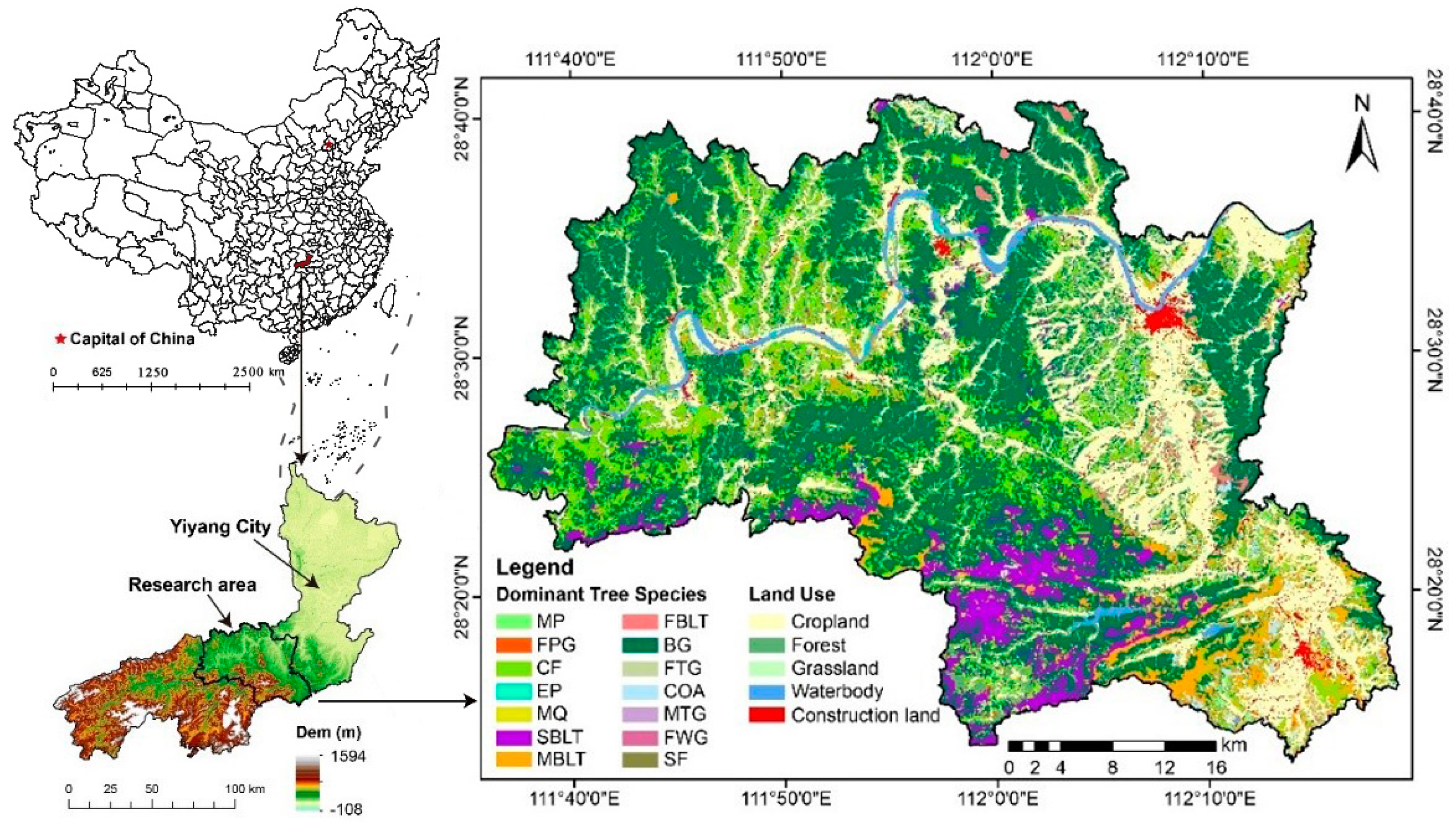
2.1. Study Area

Our study area (Taojiang County) is located in the north-central region of Hunan Province in China (Figure 1). The region is rich in subtropical forest resources, has a leading position in the county in terms of ecological economics, and ranks in the top ten in ecological forestry in Hunan. Its forest ecological benefits have received widespread attention and have been researched in the past ten years (China’s “12th Five-Year Plan” and “13th Five-Year Plan”, 2011–2021).
The total area of the study area is 2068 km2 (28°13′–28°41′ N, 111°36′–112°19′ E), and the region is characterized by a typical humid subtropical monsoon climate [17]. The topography is complex and diverse, with mostly hills in the northwest and east and plains and valleys in the middle (altitude from −108 m to 1594 m), and is mainly composed of red soil (76.34%) and yellow soil (1.18%). The forest cover rate in the study area was 62.98%, with 14 main tree species. During the “12th Five-Year Plan” period, the total amount of bamboo in the region ranked third in China and first in Hunan Province (with an area of 77,095.5 hm2 and a total of 219 million trees).

2.2. Field Data Collection

Forest field survey data (FFSD) were obtained from the Second Class of Forest Resources Survey Project in the “12th Five-Year Plan” of China from 2011 to 2015. This project is a field survey carried out by the Hunan Provincial government according to the technical regulations of forest resource surveys (GB/T26424-2010, Survey and Planning Institute of State Forestry Administration, Beijing, China, 2011). The work was completed in December 2013, and a 1:100,000–1:10,000 forest cover map of the province was established. These forest surveys and the database obtained from the survey were based on the county (city, district) as the object, and the systematic sampling method was used to establish fixed plots. In strict accordance with the technical regulations, the forest resource indexes were inventoried. All survey data were released at the end of 2014 in the forest resources monitoring system via the county-level website (http://www.taojiang.gov.cn/, accessed on 6 March 2023).
The process for establishing the plots conformed to the following criteria: (1) The forest map spots were drawn based on satellite images. Circular sample spots within the patches were established, and the size was set to 30 × 30 m (0.09 hm2). A subplot of 5 × 5 m (0.0025 hm2) was arranged at the four corners of the plot for densification. Forest age (FA), diameter at breast height (D), tree height (H), and other indexes were measured in the field. (2) Identification of representative tree species. In the sample plots, the species (group) with the most significant proportion of stock volume was the DTS (group). For young forests that had not reached the starting diameter of D and plots with unformed forest, the tree species (group) with the largest proportion of trees was the DTS (group) in the plot. (3) Arboreal forests with D ≥ 5 cm and H ≥ 1.3 m were included in the measurement range. The specific dominant tree species and features in the study area are shown in Table 1. A total of 50,482 plots were collected in the study area, and more than 1000 square kilometers of forest are involved. Masson pine (MP), Chinese fir (CF), Euramerican poplar (EP), and Metasequoia (MQ) cover more than two-thirds of the forest area.

2.3. Biomass Estimation

Based on the allometric growth equation developed for the national-scale forest ecosystem published by the “13th Five-Year Plan” National Fund project [18,19,20], we selected biomass equations with high fitting accuracy to calculate the FBs of parts of the DTS in the study area. The biomass equation coefficients of the DTS refer to the relevant references [12,18,19,21,22,23,24,25,26,27], and we use this field estimate value as measured biomass. The field observation plots were divided into two parts, one for training the model (70% of the samples) and the other for validation and evaluation of prediction accuracy (30% of the samples). The measured FB was used as the dependent variable, and the independent variables were obtained from Landsat-8 bands, forest field survey data, DEMs, and meteorological station data. The specific processing procedure is shown in Figure 2.
A total of 50,482 plots were collected in the study area, and 20,538 plots of DTS participated in RF model training and validation, including 1096 Masson pine (MP), 19,176 Chinese fir (CF), 241 European poplar (EP), and 25 metasequoias (MQ) plots. The FB by tree species can be calculated by estimating the sum of the trunk, branch, leaf, and root biomass of all trees in the plot, where aboveground biomass (AGB) equals the sum of the trunk, branch, and leaf parts and belowground biomass (BGB) refers to root biomass. Therefore, stratified random sampling was used to select 12,017/20,538 plots that met the modeling requirements (plots with D < 5 cm and H < 1 m were removed, and outliers of each regression index were eliminated).
A total of 8411 samples were used for RF model training and equation construction (trunk, branch, leaf, and root), and the remaining 3606 samples were used for the independent validation of model accuracy. The formula for the allometric growth equation is as follows:
W s = a ( D 2 H ) b
where W s refers to the biomass per tree (kg·a−1) in the sample plot; D is the average diameter at breast height (cm) of the tree species in the plot; H is the plot’s average tree height (m); and a and b are the coefficients of the allometric growth equation.
W t = a ( D 2 H ) b × Q × A
where W t refers to the total forest biomass (kg) in the sample plot; D is the average diameter at breast height (cm) of the tree species in the plot; H is the plot’s average tree height (m); a and b are the coefficients of the allometric growth equation; Q refers to the number of plants per hectare (a·hm−2); and A is the plot area (hm2).

2.4. Multispectral Indexes Based on Remote Sensing Data

This study used Landsat-8 OLI_TIRS image (30 m resolution) data from the United States Geological Survey (USGS). The images were collected on 11 October 2013, covering the entire boundary of the study area (https://www.usgs.gov/, accessed on 6 March 2023). We used the ENVI 5.3 platform to calculate the spectral vegetation index after radiometric correction and atmospheric correction of the images (http://ltpwww.gsfc.nasa.gov/. 11 October 2013). In this study, the reflectances of 8 individual bands (Coastal, Blue, Green, Red, NIR, SWIR-1, SWIR-2, and TIRS-1) and 37 spectral vegetation indexes (ARVI, DVI, EVI, GARI, GCI, GDVI, GEMI, GLI, GNDVI, GOSAVI, GRVI, GSAVI, GVI, IPVI, LAI, MNDWI, MNLI, MSAVI2, MSR, MTVI, MTVI2, NDMI, NDVI, NLI, OSAVI, PVI, RDVI, RECI, RG, SAVI, SGI, SIPI, SR, TDVI, VARI, WDRVI, and WVVI) were evaluated. The calculation methods for these spectral vegetation indexes are readily available on websites (https://www.l3harrisgeospatial.com/docs/, accessed on 6 March 2023) and the Spectral Vegetation Calculator of ENVI 5.3.
In addition, we retrieved the remote sensing ecological index (RSEI) based on the Landsat-8 TIRS band 10 (TIRS-1) and atmospheric correction parameter calculator provided on the NASA website (https://atmcorr.gsfc.nasa.gov/, accessed on 6 March 2023). The RSEI is an index based entirely on remote sensing technology that rapidly monitors and evaluates the ecological status of terrestrial ecosystems based on natural factors [28]. The index integrates four evaluation indicators using principal component analysis (PCA), including Vegetation Coverage Index (VCI), Land Surface Temperature (LST), Humidity Index (HI), and Normalized Dryness Building Soil Index (NDBSI).
P C o n e = f ( V C I , L S T , H I , N D B S I )
R S E I = 1 P C o n e 1 P C o n e m i n 1 P C o n e m a x 1 P C o n e m i n
where P C o n e refers to the ecological condition index obtained by the weighted preposition of PCA eigenvalues after standardizing four indexes ( V C I , L S T , H I , and N D B S I ). The PCA eigenvalues of each index are 0.1642, 0.0820, 0.0342, and 0.0001, respectively.
Another critical dataset is the forest canopy height (FCH) map, which is widely used for FB mapping. We used China’s 2019 canopy height data developed by Liu et al. (2022) [29]. The FCH error in the study area was corrected by referring to the global height map estimated by Simard et al. (2011) [30]. Moreover, we collected forest age (FA), living wood growing stock (LWGS), and forest canopy density (FCD) data from field survey data. In addition, digital elevation model (DEM) data with a spatial resolution of 30 m provided by the USGS were used to create three variables (elevation, slope ratio (SlopeR), and slope aspect (SlopeD)). These were combined with field survey data (geomorphic type (GT) and slope position (SlopeP)) for a total of five topographic and geomorphic indicators. All collected data were rechecked for topological errors and converted to the same coordinate system (WGS 84/UTM 49 N).

2.5. Random Forest Regression and Least Squares Fitting (RF-LS Model)

Random forest (RF) is a more advanced classification regression tree (CART) method [4], and regression models have been shown to have good predictive performance in importance identification and index clustering [31,32]. Compared with machine learning methods such as stepwise regression and support vector machines (SVMs), the RF model has outstanding advantages in terms of prediction accuracy and stability [33]. Therefore, RF models are suitable for classification and regression problems. During regression, RF generates any number of simple trees used to vote and average their responses to obtain estimates of the importance of the dependent variables. Variable data are randomly sampled via iterative bagging bootstrap sampling to generate a forest of regression trees. The basic principles of the RF model are as follows [14]:
R F p r e d i c t i o n = 1 n i = 1 i n i T r e e   r e s p o n s e
where n refers to the node of each classification tree. We used the “increase mean squared error” (IncMSE) to assign a value to each predictor randomly. If the predictor is essential, the model prediction error will increase when its value is randomly replaced. Therefore, the importance of this indicator increases as its value increases. We used “increase node purity” (IncNP) to measure the residual sum of squares to represent the effect of each indicator on the heterogeneity of the observed data at different nodes in the classification tree. The more significant the value is, the more important the corresponding variable is. For “IncMSE” or “IncNP”, one was selected as the ranking index for assessing the importance of different indicators, and the other was used as the accuracy verification index. In addition, we performed five tenfold cross-validations (CVs) and selected metrics based on the CV curve. The CV method uses different index combinations to verify the accuracy of regression models in multiple groups, which solves the problem that the test results are exceedingly one-sided and the data are insufficient. In addition, we used the Pearson correlation and significance test to further reveal the relationship between the optimal regression index and the biomass of each tree part. The RF model was run in R-Studio (version 4.1.4) [34], and the Pearson correlation and significance tests were performed using SPSS 25. Table 2 shows the details of the RF modeling groups.
Least squares (LS) is a mathematical optimization technique for finding the optimal solution by minimizing the sum of squared errors. The least squares method can also be used for curve fitting to obtain the optimization problem of the coefficients with the existing formula. After completing the RF modeling, we performed fitting optimization of the a and b coefficients of the allometric growth equation W = a ( D 2 H ) b according to the prediction results. That is, given multiple sets of data x 1 , y 1 , x 2 , y 2 , , x n , y n and formula y = a ( x ) b , the following optimal problem is solved:
min a , b n = 1 N y n a ( x ) b 2
The LS model was implemented in R-Studio (version 4.1.4) and GraphPad Prism 8. The dependent variable is the prediction result of RF modeling, and the independent variable is the product of tree diameter at breast height squared D 2 and tree height H .
We used the coefficient of determination (R2) and the root mean square error (RMSE) to quantify the performance of the model. Moreover, we used eCognition software (version 9.0) to perform multiscale supervised classification on the Landsat-8 images to identify forest land in the study area, reducing the prediction error caused by non-forest land to FB in early regression modeling and subsequent statistical analysis.

3. Results

3.1. Vertical-Scale Forest Biomass Modelling Using the Random Forest (RF) Model

We used feature importance from the Random Forest model to identify the primary indicators capable of predicting biomass. Then, we utilized the training set to assess the accuracy of these models, with the objective of minimizing errors in the prediction models (Figure 3).
As shown in Figure 3A, FCH made the greatest contribution to trunk biomass (WT), which indicated that FCH was the most important index of the WT. SoilOMC also strongly explained the WT among the soil properties. The RSEI was the remote sensing indicator with the most vital interpretation of the WT. The AEVP and MEVP were more explanatory of the WT than were the other climate factors. The importance ranking of these indicators based on “IncNP” was consistent with the ranking based on “IncMSE”, in which RECI and WDRVI showed a more substantial interpretation of WT compared to other spectral vegetation indexes. As shown in the mosaic in Figure 3A, the optimal model could be obtained by selecting the top 28−30 indicators. The overall accuracy (R2) reached 87.45%, and the mean square error (MSE) was 15.82 kg·a−1.
Thus, we performed a correlation analysis with the top 28 indicators selected by the RF model (Figure 3B) and found that FCH, RECI, SoilOMC, VARI, GLI, WDRVI, LWGS, RSEI, and NDVI exhibited a strong positive correlation with WT, while RG showed a strong negative correlation. Then, we used the training set (70% of the samples) to assess the prediction accuracy of the model (Figure 3C). The accuracy validation results showed that R2 = 0.88 and RMSE = 3.53, which were lower than the average values. The predicted values exhibited a significant correlation with the field estimate values. Therefore, the WT model exhibited good prediction accuracy according to the preliminary assessments. Similarly, we analyzed the model performance for WB, WL, and WR, and the first 19, 20, and 25 indicators were selected by the RF model, respectively. All the models showed good prediction accuracy.

3.2. FB Prediction Model Validation and Its Equation Construction

After optimal regression modeling using the RF model, we obtained four vertical-scale quantity estimation equations for WT, WB, WL, and WR through two linear and nonlinear fitting methods. Then, we used the test set to validate the accuracy of the prediction models. The test set fitting and ROC curve aim to assess the predictive stability of the biomass estimation models (Figure 4).
Figure 4 had showed the accuracy verification and prediction stability evaluation of forest biomass models using random forest method. We aggregated the WT, WB, WL, and WR to evaluate the model prediction accuracy in terms of total biomass. The AUCs of the four models were all above 0.75, and the overall prediction accuracy was 0.81, indicating that the variable prediction accuracies of the WT, WB, WL, and WR models were credible.

3.3. Optimizing Coefficients Using the Least Squares (LS) Algorithm

After building the estimation models for the vertical scales of FB using the random forest (RF) model, we introduced the least squares (LS) algorithm combined with the diameter at breast height (D) and tree height (H) indexes from the field survey and fitted coefficients a and b of the allometric growth equation ( W = a ( D 2 H ) b ) of DTS by 1000 optimization iterations. Since the construction of the prediction models was based on DTS with known parameters a and b , and our survey data includes 10 DTS with unknown a and b (Figure 5), we applied LS again to optimize the fitting of biomass estimation parameters a and b for these DTS. This aims to achieve the rapid and accurate estimation of trunk, branch, leaf, and root biomass.
As shown in Figure 5, the WT of the broad-leaved trees (SBLT, MBLT, and FBLT) exhibited a significant positive correlation with D2H and its biomass increase was weakly affected by stand age (the greater the age was, the greater the D2H), while the WB, WL, and WR of the broad-leaved tree species remained stable at D2H = 4000. As the tree grew, the biomass increased in the following order: WT > WR ≈ WB > WL. The WT growth of the bamboo group (BG) was similar to that of the broad-leaved tree species, with the order of FB increase as follows: WT > WR > WL ≈ WB. Camellia oleifera Abel (COA) differed from BG and broad-leaved tree species. The growth rate of the WT of COA exhibited a downward trend at D2H = 50, while that of its WB, WL, and WR remained unchanged after D2H = 50, which may be due to fruit growth, which affects biomass distribution at the later stage. Notably, the increase in WB in the fruit tree group (FTG) was inversely proportional to D2H at the earlier stage, possibly because of the influence of fruit growth. In addition, the increase in the WT, WB, WL, and WR of the medicinal tree group (MTG) was inversely proportional to D2H, and the biomass decline rate of each part of the tree in the early stage of growth was relatively significant and became stable after D2H = 20. The FB of the MTG declined significantly in the pre-growth stage, and the reasons for this decline need to be further studied.
In conclusion, the integrated RF-LS model can reasonably predict the FB at different vertical scales and fit the coefficients a , b for the allometric growth equations (Table 3). In addition, we found that the greater the DTS is in the plot, the better the FB inversion and fitting in the study area. Therefore, expanding the study area and collecting more ground-measured data on tree species can help to improve the fitting accuracy of the coefficients for tree species with too few sample points, which can also enhance the applicability and objectivity of the coefficients.

4. Discussion

4.1. Accuracy of the RF-LS Machine Learning Model for Forest Biomass Evaluation

The results indicated that compared with traditional biomass estimation methods, the RF-LS model we established exhibited better performance in FB inversion and simulation assessment. For example, compared with the stepwise (R2 = 0.67~0.82) [35], Leaps-BMA (R2 = 0.60~0.62) [5], and Cubist models (R2 = 0.75) [36] used by previous scholars, the RF-LS model (R2 = 0.76~0.93) we established exhibited better forest biomass (FB) prediction ability. Because the random forest (RF) model is a more advanced classification regression tree (CART) method [14], this regression model has been shown to have good predictive performance in identifying important metrics and clusters [13]. Compared with machine learning methods such as stepwise regression (stepwise) and support vector machines (SVMs), When analyzing multiple variables, these models perform better in fitting with small sample sizes, but as the sample size increases, the fitting effect will decrease. In this study, the RF model exhibits outstanding advantages in terms of prediction accuracy and stability [33,37]. Thus, the RF model is more suitable for inversion and regression problems [38]. In addition, revealing the importance of indicators based on iterative bagging bootstrap random sampling votes improves the objectivity and scientific rationale when selecting predictor indicators.
Compared with previous studies on FB estimation in subtropical forests [36,39,40], we enhanced the degree of correlation between FB and remote sensing factors. We also improved the diversity and scientific selection of indexes affecting FB inversion by integrating machine learning and remote sensing technology. Moreover, our proposed RF-LS algorithm using linear and nonlinear methods exhibited higher prediction accuracy and stability, improving the accuracy of FB inversion and regression (Table 4). We compared the biomass evaluation effect of the RF-LS model constructed in this study with that of previous studies’ models on the same tree species (above-ground biomass, AGB). The results show that the models we constructed show significant improvements in accuracy. Additionally, we noted that the FB and carbon conversion coefficient (BCTC) of the InVEST model are 0.43~0.51 [41], while the average BCTC of DTS in our study area is 0.375 (lower than the experience value of 0.43~0.5) using the model evaluation parameters of this study, which corresponds to the conclusion that general ecological models overestimate carbon storage [42]. Thus, our study was able to improve the estimation accuracy of forest carbon storage in subtropical regions.
In addition, we subdivided the aboveground biomass (AGB) into three layers (trunks, branches, and leaves) based on the vertical scale. Compared with the four-layer primary carbon pool (aboveground, belowground, soil, and humus) in the general ecological model, the comprehensive and detailed scales of AGB improve the accuracy of FB estimation and reduce the uncertainty of the empirical value assignment of the carbon pool based on different land use types. Moreover, as root biomass is a part of belowground biomass, accurate modeling dramatically reduces the error of traditional root-to-shoot ratios in estimating belowground biomass [43,44,45]. However, this study focused only on the vertical-scale FBs of subtropical forest ecosystems, and the total carbon pool needs to be further investigated [46].

4.2. Applicability of the RF-LS Machine Learning Model

This study used simple linear and nonlinear methods for constructing biomass estimation equations. From the perspective of mathematical algorithms, it is worth exploring whether multilevel mathematical formulas can improve the fitting accuracy of biomass indicators [26,47]. In addition, considering net primary productivity (NPP) and landscape pattern indexes [48,49] might also improve the interpretability of FB indicators. There were four types of dominant tree species (DTS) in the study area (CF, BG, SBLT, and MBLT), and the number of sample plots for other DTS was relatively small. The a , b coefficients of the allometric growth equations could be further optimized. However, comparative studies on stratified FBs utilizing different types of machine learning methods are lacking. Currently, both the LS-SVM [18,19,21,22,50] and the integrated RF-LS derived in this study can accurately estimate stratified FBs. In addition, the RF model used in this study, compared with other studies, shows that the number of samples trained in the model was higher compared to previous research. This may also be a reason for the improved accuracy, so we recommend that enough sample points should be collected. In any case, whether integrating multiple machine learning methods can also improve FB estimation accuracy warrants further study.
FBs include not only trunk, branch, leaf, and root biomass but also the biomass of the humus and litter layers [3,9,47,51]. Studies have noted that current models vastly overestimate regional carbon stocks [42]. The reason for this is that ecological models usually only introduce the four primary carbon pools, consider only the AGB of the forest as a whole, ignore the vertical structure of the forest, and use the empirical value of the root-to-shoot ratio to convert the belowground biomass [52,53,54]. Studies have shown that underground biomass modeling can improve the accuracy of FB evaluation [55,56,57]. Therefore, our study considered the vertical structure of the forest (trunk, branches, leaves, and roots), especially the root model, which helps to improve the accuracy of belowground biomass estimation. Although the overall accuracy reaches R2 = 0.87, the modeling accuracy of the branch biomass (R2 = 0.77) needs to be improved.

4.3. Limitations and Suggestions for Optimizing Subtropical Forest Biomass Estimation

Before selecting variables by machine learning, increasing variable diversification can enable the avoidance of the collinearity of indicators and the overfitting of models to a certain extent, which helps improve modeling accuracy and credibility [31,58]. While a fixed combination of regression models may be suitable for different forest types [59], specific parameters might vary according to the local features of tree species [60]. Previous studies have shown that hierarchical models, such as the Bayesian model (BMA), can also comprehensively consider the unique situation of each population, thus significantly improving the predictive ability of multiple regression [61]. Thus, combining different machine learning methods and selecting the optimal regression model according to a hierarchical model can help to improve the applicability and accuracy of estimating the vertical-scale FBs (trunks, branches, leaves, and roots) of forests.
The biomass of bark, litter, and humus was not considered in this study, which suggests room for optimization in FB estimation. Moreover, current research has focused more on the aboveground biomass of forests [36,62,63,64], and certain uncertainties in the estimation of belowground biomass and soil biomass still exist [42,53]. Although the RF-LS model can obtain a root biomass inversion model and fitting coefficients with high accuracy, it is insufficient for comprehensive carbon pool estimation [65]. In addition, deforestation and species expansion are key factors affecting regional biomass and carbon sequestration potential [66,67], and regional FB evaluation can be refined by considering spatiotemporal changes and scenario analysis [68,69,70,71].
More accurate estimation data can be obtained by selecting high-resolution raw data [10]. Our study used 30 m resolution primary data, and 1 m resolution remote sensing data from GF satellites might improve the inversion accuracy. However, there was a lack of remote sensing data for identifying and mapping high-precision forest-type maps during the study period (2011–2013). Nevertheless, we note that integrating advanced remote sensing techniques and machine learning algorithms into accurate inversion methods may significantly improve FB estimates in the future [72,73,74]. In addition, the diversity of regressors and the combination of machine learning methods can also improve the accuracy of FB inversion [8,75,76,77,78]. This study lacks direct measurements of biomass, as it relies on results estimated through equations, which may lead to a certain degree of verification bias, this is also a drawback of estimating biomass in large-scale studies. Although there are still challenges in obtaining and calculating high-precision data, the feasibility of this idea for large-scale FB evaluations needs to be further explored.

5. Conclusions

The main contribution of this study was to develop an RF-LS machine learning algorithm based on remote sensing and field survey data to enable the prediction of vertical-scale FBs and the optimal fitting of allometric growth equation coefficients. This method improved the accuracy of vertical-scale hierarchical FB estimation for subtropical forests in China. The results showed that the RF-LS model explained 87.48%, 76.54%, 91.94%, and 92.84% of the variance in the trunk, branch, leaf, and root biomass portions of FB, respectively, with an overall R2 = 0.89 and RMSE of 5.43 kg·a−1 and an average R2 = 0.81 and average RMSE = 1.05 kg·a−1 for the a , b coefficients of the allometric growth equation. Moreover, to better understand the reliability of our predicted FBs, we validated our models using independent test data. Compared with previous studies, the integrated RF-LS model exhibited practical application potential in FB inversion and coefficient optimization. The overall R2 of the AGB of various DTSs increased by 12.01%, and the RMSE decreased by 7.50 Mg·hm−2; the fitting RMSE and R2 of a , b tended to fluctuate with the DTS, and the R2 of the BG significantly increased by 74%. Forest canopy height (FCH), soil organic matter content (SoilOMC), and the red edge chlorophyll vegetation index (RECI) were the most critical indicators for stratified FBs. It also indicates that these indicators play a reference role in guiding the management and operation of forest carbon reservoirs. Overall, the combined remote sensing technology and machine learning algorithms can accurately retrieve vertical-scale FBs. The integrated RF-LS model could predict the vertical-scale FB well and optimize the coefficients of the allometric growth equation. In the future, we will analyze the generalizability of our results to small- to large-scale estimates and test their applicability in different geographic regions.

Supplementary Materials

The following supporting information can be downloaded at: https://www.mdpi.com/article/10.3390/f15060992/s1.

Author Contributions

Conceptualization, Methodology, Software, Investigation, Methodology, Writing—Original draft preparation, Writing—Reviewing and Editing, G.L.; Conceptualization, Methodology, Software, Investigation, Methodology, C.L.; Conceptualization, Methodology, Software, Investigation, Methodology, G.J.; Conceptualization, Methodology, Software, Investigation, Methodology, Z.H.; Writing—Original draft preparation, Writing—Reviewing and Editing, Funding, Y.H.; Investigation, Data curation, Formal analysis, Supervision, Project administration, Funding acquisition, Writing—Reviewing and Editing, W.H.; The authors G.L. and C.L. have made equal contributions. All authors have read and agreed to the published version of the manuscript.

Funding

This research was funded by the Natural Science Foundation of Hunan Province [Grant numbers:2022JJ40862], the Key Project of Hunan Education Department [Grant number: 21A0513], the Scientific Research Project of Hunan Education Department [Grant numbers 21B0235] and the Natural Science Foundation of Hunan Province [Grant number: 2020JJ4942]. This work was supported by the Key Discipline of the State Forestry Administration [Grant number: 2016-21] and the “Double First-Class” Cultivating Subject of Hunan Province [Grant number: 2018-469].

Data Availability Statement

The data that support the findings of this study are available from the corresponding author.

Conflicts of Interest

The authors declare that they have no known competing financial interests or personal relationships that could have appeared to influence the work reported in this paper.

References

  1. Ryu, S.-R.; Chen, J.; Crow, T.R.; Saunders, S.C. Available Fuel Dynamics in Nine Contrasting Forest Ecosystems in North America. Environ. Manag. 2004, 33, 87–107. [Google Scholar] [CrossRef]
  2. Baccini, A.; Walker, W.; Carvalho, L.; Farina, M.; Houghton, R.A. Response to Comment on “Tropical forests are a net carbon source based on aboveground measurements of gain and loss”. Science 2019, 363, eaat1205. [Google Scholar] [CrossRef] [PubMed]
  3. Beer, C.; Reichstein, M.; Tomelleri, E.; Ciais, P.; Jung, M.; Carvalhais, N.; Rödenbeck, C.; Arain, M.A.; Baldocchi, D.; Bonan, G.B.; et al. Terrestrial Gross Carbon Dioxide Uptake: Global Distribution and Covariation with Climate. Science 2010, 329, 834–838. [Google Scholar] [CrossRef] [PubMed]
  4. Fararoda, R.; Reddy, R.S.; Rajashekar, G.; Chand, T.R.K.; Jha, C.S.; Dadhwal, V.K. Improving forest above ground biomass estimates over Indian forests using multi source data sets with machine learning algorithm. Ecol. Inform. 2021, 65, 101392. [Google Scholar] [CrossRef]
  5. Van Pham, M.; Pham, T.M.; Viet Du, Q.V.; Bui, Q.-T.; Van Tran, A.; Pham, H.M.; Nguyen, T.N. Integrating Sentinel-1A SAR data and GIS to estimate aboveground biomass and carbon accumulation for tropical forest types in Thuan Chau district, Vietnam. Remote Sens. Appl. Soc. Environ. 2019, 14, 148–157. [Google Scholar] [CrossRef]
  6. Timothy, D.; Onisimo, M.; Cletah, S.; Adelabu, S.; Tsitsi, B. Remote sensing of aboveground forest biomass: A review. Trop. Ecol. 2016, 57, 125–132. [Google Scholar]
  7. Avitabile, V.; Herold, M.; Henry, M.; Schmullius, C. Mapping biomass with remote sensing: A comparison of methods for the case study of Uganda. Carbon Balance Manag. 2011, 6, 7. [Google Scholar] [CrossRef] [PubMed]
  8. Sousa, A.M.O.; Gonçalves, A.C.; Mesquita, P.; Marques da Silva, J.R. Biomass estimation with high resolution satellite images: A case study of Quercus rotundifolia. ISPRS J. Photogramm. Remote Sens. 2015, 101, 69–79. [Google Scholar] [CrossRef]
  9. Saatchi, S.S.; Harris, N.L.; Brown, S.; Lefsky, M.; Mitchard, E.T.A.; Salas, W.; Zutta, B.R.; Buermann, W.; Lewis, S.L.; Hagen, S.; et al. Benchmark map of forest carbon stocks in tropical regions across three continents. Proc. Natl. Acad. Sci. USA 2011, 108, 9899–9904. [Google Scholar] [CrossRef]
  10. Wang, X.C.; Wang, S.D.; Dai, L.M. Estimating and mapping forest biomass in northeast China using joint forest resources inventory and remote sensing data. J. For. Res. 2018, 29, 797–811. [Google Scholar] [CrossRef]
  11. Santoro, M.; Beaudoin, A.; Beer, C.; Cartus, O.; Fransson, J.E.S.; Hall, R.J.; Pathe, C.; Schmullius, C.; Schepaschenko, D.; Shvidenko, A.; et al. Forest growing stock volume of the northern hemisphere: Spatially explicit estimates for 2010 derived from Envisat ASAR. Remote Sens. Environ. 2015, 168, 316–334. [Google Scholar] [CrossRef]
  12. David, H.C.; Barbosa, R.I.; Vibrans, A.C.; Watzlawick, L.F.; Trautenmuller, J.W.; Balbinot, R.; Ribeiro, S.C.; Jacovine, L.A.G.; Corte, A.P.D.; Sanquetta, C.R.; et al. The tropical biomass & carbon project–An application for forest biomass and carbon estimates. Ecol. Model. 2022, 472, 110067. [Google Scholar] [CrossRef]
  13. Xing, Y.; Yue, J.P.; Guo, Z.Z.; Chen, Y.; Hu, J.; Travé, A. Large-Scale Landslide Susceptibility Mapping Using an Integrated Machine Learning Model: A Case Study in the Lvliang Mountains of China. Front. Earth Sci. 2021, 9, 15. [Google Scholar] [CrossRef]
  14. Breiman, L. Random Forest. Mach. Learn. 2001, 45, 5–32. [Google Scholar] [CrossRef]
  15. Zhu, Y.; Feng, Z.K.; Lu, J.; Liu, J.C. Estimation of Forest Biomass in Beijing (China) Using Multisource Remote Sensing and Forest Inventory Data. Forests 2020, 11, 17. [Google Scholar] [CrossRef]
  16. Lei, F.; Yu, Y.; Zhang, D.J.; Feng, L.; Guo, J.S.; Zhang, Y.; Fang, F. Water remote sensing eutrophication inversion algorithm based on multilayer convolutional neural network. J. Intell. Fuzzy Syst. 2020, 39, 5319–5327. [Google Scholar] [CrossRef]
  17. Hu, S.S.; Zhou, Y.Q.; Cen, Y. Spatial-temporal patterns of ecological changes in the Dongting Lake region and their responses to climate factors and human activities. Remote Sens. Lett. 2024, 15, 339–352. [Google Scholar] [CrossRef]
  18. Fang, J.; Yu, G.; Liu, L.; Hu, S.; Stuart Chapin, F. Climate change, human impacts, and carbon sequestration in China. Proc. Natl. Acad. Sci. USA. 2018, 115, 4015–4020. [Google Scholar] [CrossRef] [PubMed]
  19. Fang, J.; Yu, G.; Ren, X.; Liu, G.; Zhao, X. Carbon Sequestration in China’s Terrestrial Ecosystems under Climate Change—Progress on Ecosystem Carbon Sequestration from the CAS Strategic Priority Research Program. Bull. Chin. Acad. Sci. 2015, 30, 848–857. [Google Scholar] [CrossRef]
  20. Tang, X.; Zhao, X.; Bai, Y.; Tang, Z.; Wang, W.; Zhao, Y.; Wan, H.; Xie, Z.; Shi, X.; Wu, B.; et al. Carbon pools in China’s terrestrial ecosystems: New estimates based on an intensive field survey. Proc. Natl. Acad. Sci. USA 2018, 115, 4021–4026. [Google Scholar] [CrossRef]
  21. Fang, J.; Chen, A.; Peng, C.; Zhao, S.; Ci, L. Changes in Forest Biomass Carbon Storage in China Between 1949 and 1998. Science 2001, 292, 2320–2322. [Google Scholar] [CrossRef] [PubMed]
  22. Fang, J.-Y.; Wang, Z.M. Forest biomass estimation at regional and global levels, with special reference to China’s forest biomass. Ecol. Res. 2001, 16, 587–592. [Google Scholar] [CrossRef]
  23. Hossain, M.; Raqibul, M.; Siddique, H.; Akhter, M. Manual for Building Tree Volume and Biomass Allometric Equation for Bangladesh; Bangladesh Forest Department: Dhaka, Bangladesh, 2017. [Google Scholar]
  24. Liu, J.; Ni, J. Comparison of general allometric equations of biomass estimation for major tree species types in China. Quat. Sci. 2021, 41, 1169–1190. [Google Scholar]
  25. Pilli, R.; Anfodillo, T.; Carrer, M. Towards a functional and simplified allometry for estimating forest biomass. For. Ecol. Manag. 2006, 237, 583–593. [Google Scholar] [CrossRef]
  26. Viana, H.; Aranha, J.; Lopes, D.; Cohen, W.B. Estimation of crown biomass of Pinus pinaster stands and shrubland above-ground biomass using forest inventory data, remotely sensed imagery and spatial prediction models. Ecol. Model. 2012, 226, 22–35. [Google Scholar] [CrossRef]
  27. Xiang, W.; Zhou, J.; Ouyang, S.; Zhang, S.; Lei, P.; Li, J.; Deng, X.; Fang, X.; Forrester, D.I. Species-specific and general allometric equations for estimating tree biomass components of subtropical forests in southern China. Eur. J. For. Res. 2016, 135, 963–979. [Google Scholar] [CrossRef]
  28. Yuan, B.; Fu, L.; Zou, Y.; Zhang, S.; Chen, X.; Li, F.; Deng, Z.; Xie, Y. Spatiotemporal change detection of ecological quality and the associated affecting factors in Dongting Lake Basin, based on RSEI. J. Clean. Prod. 2021, 302, 126995. [Google Scholar] [CrossRef]
  29. Liu, X.; Su, Y.; Hu, T.; Yang, Q.; Liu, B.; Deng, Y.; Tang, H.; Tang, Z.; Fang, J.; Guo, Q. Neural network guided interpolation for mapping canopy height of China’s forests by integrating GEDI and ICESat-2 data. Remote Sens. Environ. 2022, 269, 112844. [Google Scholar] [CrossRef]
  30. Simard, M.; Pinto, N.; Fisher, J.B.; Baccini, A. Mapping forest canopy height globally with spaceborne lidar. J. Geophys. Res. 2011, 116, G04021. [Google Scholar] [CrossRef]
  31. Jia, G.; Hu, W.; Zhang, B.; Li, G.; Shen, S.; Gao, Z.; Li, Y. Assessing impacts of the Ecological Retreat project on water conservation in the Yellow River Basin. Sci. Total Environ. 2022, 828, 154483. [Google Scholar] [CrossRef]
  32. Zhang, J.; Zhang, N.; Liu, Y.-X.; Zhang, X.; Hu, B.; Qin, Y.; Xu, H.; Wang, H.; Guo, X.; Qian, J.; et al. Root microbiota shift in rice correlates with resident time in the field and developmental stage. Sci. China Life Sci. 2018, 61, 613–621. [Google Scholar] [CrossRef] [PubMed]
  33. Abe, D.; Inaji, M.; Hase, T.; Takahashi, S.; Sakai, R.; Ayabe, F.; Tanaka, Y.; Otomo, Y.; Maehara, T. A Prehospital Triage System to Detect Traumatic Intracranial Hemorrhage Using Machine Learning Algorithms. JAMA Netw. Open 2022, 5, e2216393. [Google Scholar] [CrossRef] [PubMed]
  34. Zhang, Z.H. Decision tree modeling using R. Ann. Transl. Med. 2016, 4, 8. [Google Scholar] [CrossRef] [PubMed]
  35. Shao, G.; Fei, S.L.; Shao, G.F. A Robust Stepwise Clustering Approach to Detect Individual Trees in Temperate Hardwood Plantations using Airborne LiDAR Data. Remote Sens. 2023, 15, 18. [Google Scholar] [CrossRef]
  36. Zhang, R.; Zhou, X.; Ouyang, Z.; Avitabile, V.; Qi, J.; Chen, J.; Giannico, V. Estimating aboveground biomass in subtropical forests of China by integrating multisource remote sensing and ground data. Remote Sens. Environ. 2019, 232, 111341. [Google Scholar] [CrossRef]
  37. Powell, S.L.; Cohen, W.B.; Healey, S.P.; Kennedy, R.E.; Moisen, G.G.; Pierce, K.B.; Ohmann, J.L. Quantification of live aboveground forest biomass dynamics with Landsat time-series and field inventory data: A comparison of empirical modeling approaches. Remote Sens. Environ. 2010, 114, 1053–1068. [Google Scholar] [CrossRef]
  38. Zeng, N.; Ren, X.; He, H.; Zhang, L.; Zhao, D.; Ge, R.; Li, P.; Niu, Z. Estimating grassland aboveground biomass on the Tibetan Plateau using a random forest algorithm. Ecol. Indic. 2019, 102, 479–487. [Google Scholar] [CrossRef]
  39. Avitabile, V.; Herold, M.; Heuvelink, G.B.M.; Lewis, S.L.; Phillips, O.L.; Asner, G.P.; Armston, J.; Ashton, P.S.; Banin, L.; Bayol, N.; et al. An integrated pan-tropical biomass map using multiple reference datasets. Glob. Change Biol. 2016, 22, 1406–1420. [Google Scholar] [CrossRef] [PubMed]
  40. Su, Y.; Guo, Q.; Xue, B.; Hu, T.; Alvarez, O.; Tao, S.; Fang, J. Spatial distribution of forest aboveground biomass in China: Estimation through combination of spaceborne lidar, optical imagery, and forest inventory data. Remote Sens. Environ. 2016, 173, 187–199. [Google Scholar] [CrossRef]
  41. Natural Capital Project. InVEST 3.14.1 User’s Guide; Natural Capital Project, Stanford University: Stanford, CA, USA, 2022. [Google Scholar]
  42. Green, J.K.; Keenan, T.F. The limits of forest carbon sequestration. Science 2022, 376, 692–693. [Google Scholar] [CrossRef]
  43. Mokany, K.; Raison, R.J.; Prokushkin, A.S. Critical analysis of root: Shoot ratios in terrestrial biomes. Glob. Change Biol. 2006, 12, 84–96. [Google Scholar] [CrossRef]
  44. Saint-André, L.; M’Bou, A.T.; Mabiala, A.; Mouvondy, W.; Jourdan, C.; Roupsard, O.; Deleporte, P.; Hamel, O.; Nouvellon, Y. Age-related equations for above- and below-ground biomass of a Eucalyptus hybrid in Congo. For. Ecol. Manag. 2005, 205, 199–214. [Google Scholar] [CrossRef]
  45. Wang, X.; Fang, J.; Zhu, B. Forest biomass and root–shoot allocation in northeast China. For. Ecol. Manag. 2008, 255, 4007–4020. [Google Scholar] [CrossRef]
  46. Ali, A.; Yan, E.-R. Functional identity of overstorey tree height and understorey conservative traits drive aboveground biomass in a subtropical forest. Ecol. Indic. 2017, 83, 158–168. [Google Scholar] [CrossRef]
  47. Ogawa, K. Mathematical consideration of the age-related decline in leaf biomass in forest stands under the self-thinning law. Ecol. Model. 2018, 372, 64–69. [Google Scholar] [CrossRef]
  48. Tang, G.P.; Beckage, B.; Smith, B.; Miller, P.A. Estimating potential forest NPP, biomass and their climatic sensitivity in New England using a dynamic ecosystem model. Ecosphere 2010, 1, 20. [Google Scholar] [CrossRef]
  49. Singh, K.K.; Bianchetti, R.A.; Chen, G.; Meentemeyer, R.K. Assessing effect of dominant land-cover types and pattern on urban forest biomass estimated using LiDAR metrics. Urban Ecosyst. 2017, 20, 265–275. [Google Scholar] [CrossRef]
  50. Pelckmans, K.; Suykens, J.A.K.; Van Gestel, T.; De Brabanter, J.; Lukas, L.; Hamers, B.; De Moor, B.; Vandewalle, J. LS-SVMlab: A Matlab/C Toolbox for Least Squares Support Vector Machines. 2002. Available online: http://www.esat.kuleuven.be/sista/lssvmlab (accessed on 17 April 2022).
  51. Clark, D.B.; Kellner, J.R. Tropical forest biomass estimation and the fallacy of misplaced concreteness. J. Veg. Sci. 2012, 23, 1191–1196. [Google Scholar] [CrossRef]
  52. Levy, P.E. Biomass expansion factors and root: Shoot ratios for coniferous tree species in Great Britain. Forestry 2004, 77, 421–430. [Google Scholar] [CrossRef]
  53. Li, Z.; Kurz, W.A.; Apps, M.J.; Beukema, S.J. Belowground biomass dynamics in the Carbon Budget Model of the Canadian Forest Sector: Recent improvements and implications for the estimation of NPP and NEP. Can. J. For. Res. 2003, 33, 126–136. [Google Scholar] [CrossRef]
  54. Sharp, R.; Tallis, H.T.; Ricketts, T.; Guerry, A.D.; Wood, S.A.; Chaplin-Kramer, R.; Nelson, E.; Ennaanay, D.; Wolny, S.; Olwero, N.; et al. InVEST User’s Guide; Version 3.2.0; The Natural Capital Project, Stanford University: Stanford, CA, USA; University of Minnesota: Minneapolis, MN, USA; The Nature Conservancy: Arlington, VA, USA; World Wildlife Fund: Gland, Switzerland, 2014; pp. 25–353. [Google Scholar] [CrossRef]
  55. Cronan, C.S. Belowground biomass, production, and carbon cycling in mature Norway spruce, Maine, U.S.A. Can. J. For. Res. 2003, 33, 339–350. [Google Scholar] [CrossRef]
  56. Kurz, W.A.; Beukema, S.J.; Apps, M.J. Estimation of root biomass and dynamics for the carbon budget model of the Canadian forest sector. Can. J. For. Res. 1996, 26, 1973–1979. [Google Scholar] [CrossRef]
  57. Luo, Y.; Wang, X.; Zhang, X.; Booth, T.H.; Lu, F. Root:shoot ratios across China’s forests: Forest type and climatic effects. For. Ecol. Manag. 2012, 269, 19–25. [Google Scholar] [CrossRef]
  58. Hu, W.; Li, G.; Li, Z. Spatial and temporal evolution characteristics of the water conservation function and its driving factors in regional lake wetlands—Two types of homogeneous lakes as examples. Ecol. Indic. 2021, 130, 108069. [Google Scholar] [CrossRef]
  59. Asner, G.P.; Mascaro, J.; Anderson, C.; Knapp, D.E.; Martin, R.E.; Kennedy-Bowdoin, T.; van Breugel, M.; Davies, S.; Hall, J.S.; Muller-Landau, H.C.; et al. High-fidelity national carbon mapping for resource management and REDD+. Carbon Balance Manag. 2013, 8, 7. [Google Scholar] [CrossRef] [PubMed]
  60. Qian, S.S.; Chaffin, J.D.; DuFour, M.R.; Sherman, J.J.; Golnick, P.C.; Collier, C.D.; Nummer, S.A.; Margida, M.G. Quantifying and Reducing Uncertainty in Estimated Microcystin Concentrations from the ELISA Method. Environ. Sci. Technol. 2015, 49, 14221–14229. [Google Scholar] [CrossRef] [PubMed]
  61. Yun, J.; Qian, S.S. A Hierarchical Model for Estimating Long-Term Trend of Atrazine Concentration in the Surface Water of the Contiguous U.S. JAWRA J. Am. Water Resour. Assoc. 2015, 51, 1128–1137. [Google Scholar] [CrossRef]
  62. Mitchard, E.T.A.; Saatchi, S.S.; Lewis, S.L.; Feldpausch, T.R.; Gerard, F.F.; Woodhouse, I.H.; Meir, P. Comment on ‘A first map of tropical Africa’s above-ground biomass derived from satellite imagery’. Environ. Res. Lett. 2011, 6, 049001. [Google Scholar] [CrossRef]
  63. Temesgen, H.; Affleck, D.; Poudel, K.; Gray, A.; Sessions, J. A review of the challenges and opportunities in estimating above ground forest biomass using tree-level models. Scand. J. For. Res. 2015, 30, 326–335. [Google Scholar] [CrossRef]
  64. Yu, Y.; Saatchi, S. Sensitivity of L-Band SAR Backscatter to Aboveground Biomass of Global Forests. Remote Sens. 2016, 8, 522. [Google Scholar] [CrossRef]
  65. Eisfelder, C.; Klein, I.; Bekkuliyeva, A.; Kuenzer, C.; Buchroithner, M.F.; Dech, S. Above-ground biomass estimation based on NPP time-series − A novel approach for biomass estimation in semi-arid Kazakhstan. Ecol. Indic. 2017, 72, 13–22. [Google Scholar] [CrossRef]
  66. Bhattarai, T.; Skutsch, M.; Midmore, D.; Shrestha, H.L. Carbon Measurement: An Overview of Forest Carbon Estimation Methods and the Role of Geographical Information System and Remote Sensing Techniques for REDD+ Implementation. J. For. Livelihood 2016, 13, 69–86. [Google Scholar] [CrossRef]
  67. Yuan, Z.; Ali, A.; Wang, S.; Wang, X.; Lin, F.; Wang, Y.; Fang, S.; Hao, Z.; Loreau, M.; Jiang, L. Temporal stability of aboveground biomass is governed by species asynchrony in temperate forests. Ecol. Indic. 2019, 107, 105661. [Google Scholar] [CrossRef] [PubMed]
  68. Azevedo, J.C.; Perera, A.H.; Pinto, M.A. Forest Landscapes and Global Change; Springer: New York, NY, USA, 2014. [Google Scholar]
  69. Pan, Y.; Luo, T.; Birdsey, R.; Hom, J.; Melillo, J. New Estimates of Carbon Storage and Sequestration in China’s Forests: Effects of Age-Class and Method On Inventory-Based Carbon Estimation. Clim. Change 2004, 67, 211–236. [Google Scholar] [CrossRef]
  70. Zarin, D.J.; Harris, N.L.; Baccini, A.; Aksenov, D.; Hansen, M.C.; Azevedo-Ramos, C.; Azevedo, T.; Margono, B.A.; Alencar, A.C.; Gabris, C.; et al. Can carbon emissions from tropical deforestation drop by 50% in 5 years? Glob. Change Biol. 2016, 22, 1336–1347. [Google Scholar] [CrossRef] [PubMed]
  71. Zhang, H.; Song, T.; Wang, K.; Wang, G.; Liao, J.; Xu, G.; Zeng, F. Biogeographical patterns of forest biomass allocation vary by climate, soil and forest characteristics in China. Environ. Res. Lett. 2015, 10, 044014. [Google Scholar] [CrossRef]
  72. Avitabile, V.; Camia, A. An assessment of forest biomass maps in Europe using harmonized national statistics and inventory plots. For. Ecol. Manag. 2018, 409, 489–498. [Google Scholar] [CrossRef] [PubMed]
  73. Fahey, T.J.; Woodbury, P.B.; Battles, J.J.; Goodale, C.L.; Hamburg, S.P.; Ollinger, V.S.; Woodall, C.W. Forest carbon storage: Ecology, management, and policy. Front. Ecol. Environ. 2010, 8, 245–252. [Google Scholar] [CrossRef]
  74. Piao, S.; He, Y.; Wang, X.; Chen, F. Estimation of China’s terrestrial ecosystem carbon sink: Methods, progress and prospects. Sci. China Earth Sci. 2022, 65, 641–651. [Google Scholar] [CrossRef]
  75. Du, L.; Zhou, T.; Zou, Z.; Zhao, X.; Huang, K.; Wu, H. Mapping Forest Biomass Using Remote Sensing and National Forest Inventory in China. Forests 2014, 5, 1267–1283. [Google Scholar] [CrossRef]
  76. Guo, Z.; Hu, H.; Li, P.; Li, N.; Fang, J. Spatio-temporal changes in biomass carbon sinks in China’s forests from 1977 to 2008. Sci. China Life Sci. 2013, 56, 661–671. [Google Scholar] [CrossRef] [PubMed]
  77. Guo, Z.; Fang, J.; Pan, Y.; Birdsey, R. Inventory-based estimates of forest biomass carbon stocks in China: A comparison of three methods. For. Ecol. Manag. 2010, 259, 1225–1231. [Google Scholar] [CrossRef]
  78. Ningthoujam, R.K.; Joshi, P.K.; Roy, P.S. Retrieval of forest biomass for tropical deciduous mixed forest using ALOS PALSAR mosaic imagery and field plot data. Int. J. Appl. Earth Obs. Geoinf. 2018, 69, 206–216. [Google Scholar] [CrossRef]
Figure 1. Overview of the study area. The figure shows the study area located in Yiyang City, Hunan Province, China. Landsat−8 (30 m resolution) remote sensing image of the study area, with a combination of bands 4,3,2. Spatial distribution of the dominant tree species (DTS) and land use types in the study area. See Table 1 for the names of the DTS corresponding to the codes.
Forests 15 00992 g001
Figure 2. Research technology framework. (A) Calculation of biomass based on the existing allometric growth equation; (B) Inversion of biomass based on remote sensing and geoscience data using the RF model, of which 70% of the forest field survey sample plots were used for modeling and 30% for model validation; (C) Use of the inversion biomass model to estimate the overall biomass and classification statistics according to different tree species; (D) Fitting and optimization of the coefficients a and b of the allometric growth equation ( W = a ( D 2 H ) b ) for different dominant tree species (DTS) based on diameter at breast height (D) and tree height (H) measured in the field.
Forests 15 00992 g002
Figure 3. Inversion and modeling of forest vertical biomass (WT, WB, WL, and WR) based on the RF model. (A) Importance of WT, WB, WL, and WR indexes and optimal regression variables selected by the RF model; the mosaic graph refers to the results of five times tenfold cross-validation. “IncMSE” refers to the increased mean square error, and “IncNP” refers to the increased node purity of the decision tree. (B) Pearson correlation between the selected optimal regressors of WT, WB, WL, and WR. (C) Prediction accuracy verification of the forest vertical biomass model (training set, a total of 8411 samples). WT, WB, WL, and WR refer to the trunk, branch, leaf, and root biomass.
Forests 15 00992 g003
Figure 4. Accuracy verification and prediction stability evaluation of forest biomass (FB) models using random forest method and equations for the trunk (WT), branches (WB), leaf (WL), and root (WR) biomasses. We used 30% of the original dataset as the test set (3606 samples) to reevaluate the RF modeling accuracy. We used the ROC curve to evaluate the stability of the model prediction results and selected the sample plots according to different age classes (yr) of different DTS (<20, 20–40, 40–60, >60). The AUC represents the area under the ROC curve and the coordinate axis. Its value is 0.5~1. The closer the AUC is to 1.0, the higher the authenticity of the detection method is. SD refers to the root mean square error. Meas, measured biomass; Pred, predicted biomass.
Forests 15 00992 g004
Figure 5. Fitting and optimization of coefficients for allometric growth equations. The figure shows the fitting and optimization results of the allometric growth equations’ coefficients a, b for 10 dominant tree species (except for 4 types of dominant tree species involved in RF modeling), divided into the vertical scales of trunk, branch, leaf, and root. The independent variable was the product of the diameter at breast height (D, cm) squared and the tree height (H, m), and the independent variable was the biomass of the dominant tree species per plant (kg·a−1). See Table 1 for the names of the dominant trees and the detailed regression parameters.
Forests 15 00992 g005
Table 1. Information and characteristics of DTS in the study area.
IDDTS NameCharacteristicsParameters
MPMasson pineThe trunk of MP is straight; the branches spread flat or obliquely; the crown is a broad tower or umbrella; the bark is dark brown and flaky, containing resin and water, and is humidity resistant. It is the leading timber tree species in South China, with high economic value.D = 2~28 cm
n = 1096
a = 1834.6 hm2
CFChina firCF is a kind of evergreen tree with a straight trunk. The tree crown is conical, and the bark is greyish brown. The branches are flat and spreading. It mainly grows in South and East China. It is a unique tree species in China and a national first-class protected plant.D = 3~41 cm
n = 19176
a = 1834.6 hm2
EPEuramerican poplarEP is an evergreen, deciduous, fast-growing tree with high-quality wood. It has a tall tree body and the trunk is straight. The crown is narrow, and the branch angle is slight with delicate collateral branching. The leaves are small, dense, and full-crested.D = 3~28 cm
n = 241
a = 360.2 hm2
MQMetasequoiaMQ is a deciduous tree with a straight and tall trunk. The branches are drooping, brown, or brownish-grey. The surface of the branches is smooth, and the crown is steeple-shaped. It is mainly distributed in parts of South China, East China, and North China.D = 2~32 cm
n = 25
a = 7.3 hm2
SBLTSlow-growing
broad-leaved tree
A forest of slow-growth broad-leaved tree species. It mainly grows in tropical and subtropical regions and is composed of Oak, Camphor, Beech, etc.D = 4~35 cm
n = 2598
a = 10097.6 hm2
MBLTMedium-growing broad-leaved treeA forest of medium-growth broad-leaved tree species. It mainly grows in tropical and subtropical regions and includes Schima, Sassafras, etc.D = 2~51 cm
n = 5501
a = 10722.8 hm2
FBLTFast-growing
broad-leaved tree
A forest of fast-growing broad-leaved tree species. It mainly occurs in tropical regions, and in subtropical regions to a lesser extent, and mainly includes Sweet Gum, Paulownia, and Melia azedarach.D = 4~24 cm
n = 738
a = 1545.9 hm2
BG
(MB)
Bamboo group
(mainly Moso bamboo)
MB belongs to the evergreen forests of bamboo plants; it has a height of up to more than 20 m, a diameter at breast height of up to more than 20 cm, concentrated dense roots, and fast-growing bamboo stalk. It is one of the most important bamboo species in China with a long history, the largest area, and the most important economic value.D = 2~24 cm
n = 20114
a = 77361.8 hm2
COACamellia oleifera AbelCOA is a small evergreen tree. It is also a unique woody vegetable oil resource. The height ranges from 3 m to 6 m, and the diameter at breast height ranges from 24 cm to 30 cm. The bark is smooth and greyish-brown.D = 0.5~15 cm
n = 735
a= 1476.8 hm2
FPG
(PE + PT)
Foreign pine group (Pinus elliottii +
Pinus taeda)
PE and PT are fast-growing evergreen trees, native to the southeast coast of North America, Cuba, and Central America. They prefer an altitude of 150–500 m and moist soil. The height reaches up to 30 m and the diameter at breast height is up to 90 cm. The bark is greyish-brown or dark reddish-brown, and the branches are thick and orange–brown.D = 8~22 cm
n = 76
a = 155.5 hm2
FTGFruit tree groupFTP is a general term for trees with edible fruits and perennial plants that provide edible fruits, seeds, and wood, including apple trees, pear trees, citrus trees, almond trees, etc.D = 1~26 cm
n = 64
a = 113.9 hm2
MTGMedicinal tree groupBranches, bark, and fruit with particular medicinal value, such as Ginkgo, Eucommia ulmoides, Phellodendri, etc.D = 1~10 cm
n = 10
a = 18.8 hm2
FWGFlowers wood groupFWG can be divided into herbaceous flowers, woody flowers, and aquatic flowers. Herbaceous flowers have soft stems; woody flowers have stiff woody stems. It includes Osmanthus, Camphor, etc. They are mainly used for landscaping.D = 1~18 cm
n = 43
a = 36.7 hm2
SFShrubs fernsSF refers to a short, densely clustered tree, not more than 6 m tall, without an obvious trunk, generally broad-leaved, but some conifers are shrubs.D = 1~10 cm
n = 13
a = 25.5 hm2
Note: DTS, dominant tree species; ID, abbreviations of tree species; D, tree diameter (cm); n, number of sample points; a, area of sample points.
Table 2. Biomass regression indexes based on random forest model.
IndicatorsData Sources and Preprocess MethodsFormat
Landsat-8 bands (8)Landsat-8 bands were derived from the OLI_TIRS images (USGS). Remote sensing images of the study area in October 2013 were selected with a resolution of 30 m and a cloud cover of less than 5%. ENVI 5.3 software was used for atmospheric correction and radiometric calibration. We selected band-1 (Coastal), band-2 (Blue), band-3 (Green), band-4 (Red), band-5 (NIR), band-6 (SWIR-1), band-7 (SWIR-2), and band-10 (TIRS-1), for a total of 8 bands
(https://www.usgs.gov/, accessed on 6 March 2023).
Tiff
Spectral vegetation indexes (37)Spectral vegetation indexes were based on the image bands after atmospheric correction and radiometric calibration of Landsat-8 images. They were obtained using the band calculator of ENVI 5.3 software, and included 37 indexes: ARVI, DVI, EVI, GARI, GCI, GDVI, GEMI, GLI, GNDVI, GOSAVI, GRVI, GSAVI, GVI, IPVI, LAI, MNDWI, MNLI, MSAVI2, MSR, MTVI, MTVI2, NDMI, NDVI, NLI, OSAVI, PVI, RDVI, RECI, RG, SAVI, SGI, SIPI, SR, TDVI, VARI, WDRVI, and WV-VI.
(https://www.l3harrisgeospatial.com/docs/, accessed on 6 March 2023).
Tiff
Ecological indexes (10)Ecological indexes reflect the advantages and disadvantages of the regional ecological environment and are calculated based on the image bands and vegetation indexes preprocessed by Landsat-8 images using the principal component analysis and weighted overlay tool of ENVI 5.3 software. We selected a total of 10 indicators, including RSEI, SRRI, BRII, GSTI, HI, SI, IBI, NDBSI, PCone, and VCI. See Formulas (3)–(6) in Section 2.4 for specific formulas and indexes.Tiff
Geographical indicators (5)Geographical indicators data were calculated by DEM with 30 m resolution downloaded from the USGS. It contains five parameters: geomorphic types (GT), slope ratio (SlopeR, °), slope aspect (SlopeD), elevation (m), and slope position (SlopeP) (https://www.usgs.gov/, accessed on 6 March 2023).Tiff
Soil properties (2)Soil properties data were obtained from the China Soil Dataset (V1.2) in the World Soil Database, and we selected two soil indexes: soil depth (SoilDEP, cm) and soil organic matter content (SoilOMC, mg/100 g)
(https://iiasa.ac.at/models-and-data/harmonized-world-soil-database, accessed on 6 March 2023).
Tiff
Climate indicators (30)Climate indicators were derived from the daily dataset (TXT format) of the China Meteorological Administration. The data from 24 meteorological stations in the study area and its surrounding areas were selected, processed, and interpolated using the inverse distance weighting (IDW) method in R-Studio (4.3) and ArcGIS (10.1) and integrated into three kinds of data: annual average (AA), monthly average (MA), and daily average (DA), including the precipitation (PCP, mm), evaporation (EVP, mm), average temperature (TEM, °C), temperature change (TC, °C), solar radiation (RAD, MJ), solar duration hours (SDH, h), surface temperature (ST, °C), atmospheric pressure (AP, pa), relative humidity (RH, %), and wind speed (WS, m/s), for a total of 10 indexes(https://www.data.cma.cn/, accessed on 6 March 2023). Shape/Tiff
Tree growth indexes (4)Tree growth indexes were derived from field survey data and research data from previous studies, including forest age (yr), canopy density (%), living wood growing stock (m3/hm2), and canopy height (m) [29,30]
(http://www.taojiang.gov.cn/, accessed on 6 March 2023).
Shape/Tiff
Note: Some supplementary statements are provided in Section 2.4, and detailed index names and calculation formulas are provided in Supplementary Appendix 1.
Table 3. Optimization of coefficients of allometric growth equations for dominant tree species.
IDDTS NameScaleabR2RMSEApp
SLBTSlow-growing broad-leaved treeTrunk0.46300.54910.854.06D = 4~35 cm
n = 2598
Branch0.07640.57480.870.76
Leaf0.17740.42680.860.48
Root0.23230.45770.880.73
MLBTMedium-growing broad-leaved treeTrunk0.34180.57190.913.23D = 2~51 cm
n = 5501
Branch0.13860.48400.810.87
Leaf0.11630.46590.850.56
Root0.20390.46580.890.79
FLBTFast-growing broad-leaved treeTrunk0.06880.77120.883.59D = 4~24 cm
n = 738
Branch0.03970.63230.790.86
Leaf0.01760.70060.860.55
Root0.06550.60790.890.77
BGBamboo group
(mainly Moso bamboo, MB)
Trunk0.12450.71950.912.35D = 2~24 cm
n = 20,034
Branch0.02790.68620.890.44
Leaf0.02650.68130.880.42
Root0.07440.61170.850.70
COACamellia oleifera AbelTrunk8.82810.20570.832.06D = 1~15 cm
n = 580
Branch2.88700.13740.670.66
Leaf1.04710.25700.840.33
Root3.08010.14460.830.39
FPGForeign pine group
(mainly Pinus elliottii + Pinus taeda)
Trunk1.16300.40360.941.69D = 8~22 cm
n = 73
Branch1.86710.15590.610.71
Leaf0.19000.39390.870.41
Root0.62080.30140.820.62
FTGFruit tree groupTrunk8.03200.14240.762.17D = 3~26 cm
n = 60
Branch4.1351−0.03300.261.24
Leaf0.80840.19510.690.54
Root2.95700.08280.750.46
MTGMedicinal tree groupTrunk17.501−0.09530.831.19D = 1~10 cm
n = 10
Branch3.7660−0.12520.950.15
Leaf2.3071−0.05450.740.15
Root4.6520−0.06190.780.32
FWGFlowers wood groupTrunk6.84100.19170.821.97D = 1~18 cm
n = 43
Branch1.09410.21990.790.45
Leaf0.91550.19910.750.36
Root2.81300.11280.780.37
SFShrubs fernsTrunk12.3500.12220.772.45D = 1~10 cm
n = 13
Branch1.54700.24220.740.82
Leaf1.62410.16090.650.58
Root2.38900.11340.640.74
Note: DTS, dominant tree species; ID, abbreviations of tree species; D, diameter at breast height (cm); n, number of sample points; R2, fitting accuracy; RMSE, root mean square error; App, applicability of models. The equation is W = a ( D 2 H ) b .
Table 4. Comparison of aboveground biomass prediction models of subtropical forests in different studies.
R2RMSE (Mg·hm−2)
Forest TypeSu (2016)Avitabile (2016)Zhang (2019)This StudyZhang (2019)This Study
CF0.110.210.760.8662.750.5
MP0.050.290.770.7939.435.2
FBLT0.230.230.760.8252.950.1
MBLT0.100.200.750.8553.346.7
SBLT0.140.310.710.8158.252.9
BG0.010.200.140.88-32.2
MQ0.250.460.670.7682.754.3
Overall--0.750.8754.046.5
Note: Su (2016) refers to [40]; Avitabile (2016) refers to [39]; and Zhang (2019) refers to [36]. Comparison according to aboveground biomass (AGB = WT + WB + WL).
Disclaimer/Publisher’s Note: The statements, opinions and data contained in all publications are solely those of the individual author(s) and contributor(s) and not of MDPI and/or the editor(s). MDPI and/or the editor(s) disclaim responsibility for any injury to people or property resulting from any ideas, methods, instructions or products referred to in the content.

