Mapping Forest Stock Volume Using Phenological Features Derived from Time-Serial Sentinel-2 Imagery in Planted Larch

Abstract

As one of the important types of forest resources, mapping forest stock volume (FSV) in larch (Larix decidua) forests holds significant importance for forest resource management, carbon cycle research, and climate change monitoring. However, the accuracy of FSV mapping using common spectral and texture features is often limited due to their failure in fully capturing seasonal changes and growth cycle characteristics of vegetation. Phenological features can effectively provide essential information regarding the growth status of forests. In this study, multi-temporal Sentinel-2 satellite imagery were initially acquired in the Wangyedian Forest Farm in Chifeng City, Inner Mongolia. Subsequently, various phenological features were extracted from time series variables constructed by Gaussian Process Regression (GPR) using Savitzky–Golay filters, stepwise differentiation, and Fourier transform techniques. The alternative features were further refined through Pearson’s correlation coefficient analysis and the forward selection algorithm, resulting in six groups of optimal subsets. Finally, four models including the Random Forest (RF), K-Nearest Neighbors (KNN), Support Vector Machine (SVM), and Multiple Linear Regression (MLR) algorithms were developed to estimate FSV. The results demonstrated that incorporating phenological features significantly enhanced model performance, with the SVM model exhibiting the best performance—achieving an R² value of 0.77 along with an RMSE value of 46.36 m³/hm² and rRMSE value of 22.78%. Compared to models without phenological features, inclusion of these features led to a 0.25 increase in R² value while reducing RMSE by 10.40 m³/hm² and rRMSE by 5%. Overall, integration of phenological feature variables not only improves the accuracy of larch forest FSV mapping but also has potential implications for delaying saturation phenomena.

1. Introduction

Larch (Larix decidua) grows mainly in temperate and sub-boreal regions of the Northern Hemisphere, especially in high-altitude mountainous areas and higher northern latitudes [1]. Researchers like Duan Beixing have revealed the significant drought resistance and vitality exhibited by larches. This species can grow in poor soil conditions, playing a crucial role in maintaining local ecological balance [2,3]. With the escalating global climate change, larch (Larix decidua), an important and widely distributed tree species, shows significant spatiotemporal variations in its distribution, growth, and biomass accumulation. As a species with excellent timber properties and important ecological functions, monitoring the dynamics of larch is essential for understanding its role in the global carbon cycle, guiding forest management strategies and protecting biodiversity [4]. In this context, accurate mapping forest stock volume is critical for forest resource management, ecosystem protection, and research on the global carbon cycle. Therefore, precise monitoring of larch forest stock volume is vital for sustainable forest management, providing a scientific basis for forestry harvesting, renewal, and protection strategies, and playing a key role in assessing and maintaining ecosystem diversity and stability.

Currently, the application of remote sensing inversion technology for forest stock volume has reached a state of maturity [5]. Optical remote sensing data, characterized by its multi-temporal, multi-resolution, and multi-spectral advantages as well as ease of acquisition, has been extensively employed in mapping forest stock volume [6,7,8]. This approach primarily relies on satellite platforms such as Landsat, MODIS, and Sentinel-2 to provide multispectral and hyperspectral images [9,10]. By processing these images, key remote sensing features including spectral variables, vegetation indexes, and texture variables are widely extracted to construct models based on statistical relationships with ground-measured data [11,12,13,14]. However, traditional features have certain limitations. For instance, atmospheric conditions, land cover types, and observation angles can affect conventional remote sensing features and subsequently impact estimation accuracy. Moreover, such features often fail to fully capture seasonal changes and growth cycle characteristics of vegetation, restricting their effectiveness in applications involving phenological variations.

Phenological features, such as the onset, peak, and decline phases of vegetation growth, can effectively provide crucial information regarding the growth status of vegetation and ecosystem functions [15,16,17,18]. The incorporation of phenological features has introduced a novel perspective in the realm of forest resource monitoring. For instance, Zhang Yali et al. have enhanced the accuracy of estimating forest aboveground biomass by integrating phenological features [19]. In comparison to traditional remote sensing features, phenological characteristics more accurately depict seasonal changes and growth cycles of vegetation, thereby augmenting the precision of forest resource monitoring. However, several challenges still exist in applying phenological features for mapping FSV, including accurate extraction techniques for these features, handling noise in large-scale spatial applications, and addressing universality issues across different tree species.

To address these challenges, researchers have developed various methodologies for extracting phenological features, encompassing time series analysis, machine learning algorithms, and model-based approaches [20,21,22]. Time series analysis leverages remote sensing data collected at consecutive time points to discern crucial phenological stages (SOS, LOS, EOS) by scrutinizing the trends in vegetation indices over time. Machine learning algorithms enable the processing of extensive datasets and facilitate the extraction of phenological features by discerning patterns within the data. Model-based approaches aim to simulate vegetation growth processes based on ecological principles, thereby enabling the extraction of phenological features.

To improve the accuracy of mapping FSV in larch forests, this study first examines the limitations of existing single methods for extracting phenological features, and then presents a method that integrates time series analysis with ecological modeling to predict vegetation growth. Utilizing the Sentinel-2 satellite remote sensing platform, spectral variables, vegetation indices, and texture features are extracted from time series remote sensing images. Subsequently, the Gaussian Process Regression (GPR) algorithm is employed to smoothen and reconstruct the features extracted from the remote sensing data, aiming to eliminate data noise. To assess the potential of phenological features in mapping the Forest Stock Volume (FSV) in planted larch forests, various types of phenological features are extracted from time series images using three methods, namely Savitzky–Golay filtering, stepwise differentiation, and Fourier transform. Additionally, four machine learning models—Random Forest (RF), K-Nearest Neighbors (KNN), Support Vector Machine (SVM), and Multiple Linear Regression (MLR)—are applied to construct models with the optimal subset derived from the Forward Selection algorithm. The objective is to effectively identify the key phenological stages of vegetation and accurately map the FSV in planted larch forests.

2. Study Area and Data

2.1. Study Area

The study area is located in the Wangyedian Forest Farm, situated in the southwestern part of Karakin Banner, Chifeng City, Inner Mongolia Autonomous Region (Figure 1) [23]. The geographic coordinates of the forest farm range from 118°09′ to 118°30′ east longitude and 41°21′ to 41°39′ north latitude, respectively. This region predominantly comprises mid-mountain and low-mountain landscapes, with an average altitude ranging from 800 m to 1890 m. The topography exhibits higher elevations towards the southwest, gradually declining towards the northeast. Through a comprehensive investigation and statistical analysis of forest resources within Wangyedian Forest, it was determined that the total forest cover spans approximately 350,000 mu, out of which plantation forests account for around 176,000 mu. Notably, key species such as Larch plantations (Larix principis-rupprechtii), Chinese pine plantations (Pinus tabuliformis), natural secondary Dahurian birch forests (Betula dahurica), and natural secondary silver birch forests (Betula platyphylla) constitute the primary forest resources.

2.2. Ground Measured Data

In this study, the randomized stratified sampling method [24] was employed to establish ground measured samples based on the distribution of forest volume in planted larch forests. A total of 79 samples were established between October 2017 and September 2019. Each sample has a size of 25 m × 25 m. The position and angles of the center are precisely measured using GNSS, with an error margin of less than 10 cm. Within each sample, various parameters including tree height (H/m), diameter at breast height (D/cm), and crown diameter (C/m) were measured. Additionally, elevation, slope, and aspect were also recorded at the center of each sample plot. Based on the ground measured height and DBH of each tree, the volume of the individual trees was calculated using a binary volume table according to the following formula below, quantifying the relationships among diameter at breast height (DBH), tree height, and volume of larch. The special formula is expressed as follows:

$$V=-0.001498+0.00007\times D^2+0.000901\times H+0.000032\times H\times D^2$$

(1)

where D is the diameter at breast height of a single tree and H is the height of a single tree. The forest stem volume of the sample was determined by summing the volumes of all trees within the sample. The average diameter at breast height (DBH) of larch ranged from 6.18 to 29.21 cm, while the average height ranged from 5.86 to 23.70 m (Figure 2).

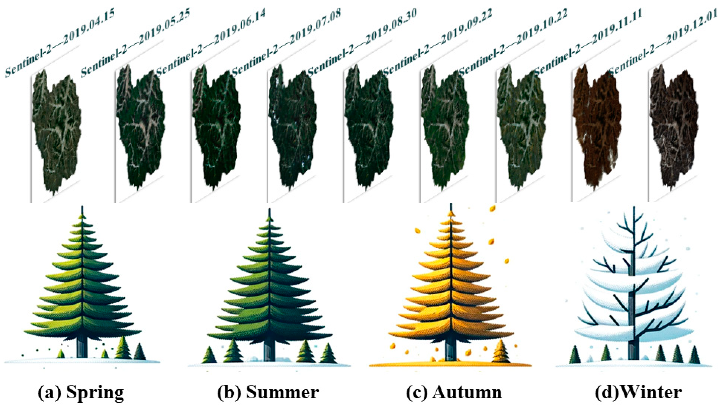
2.3. Time Series Sentinel-2 Data

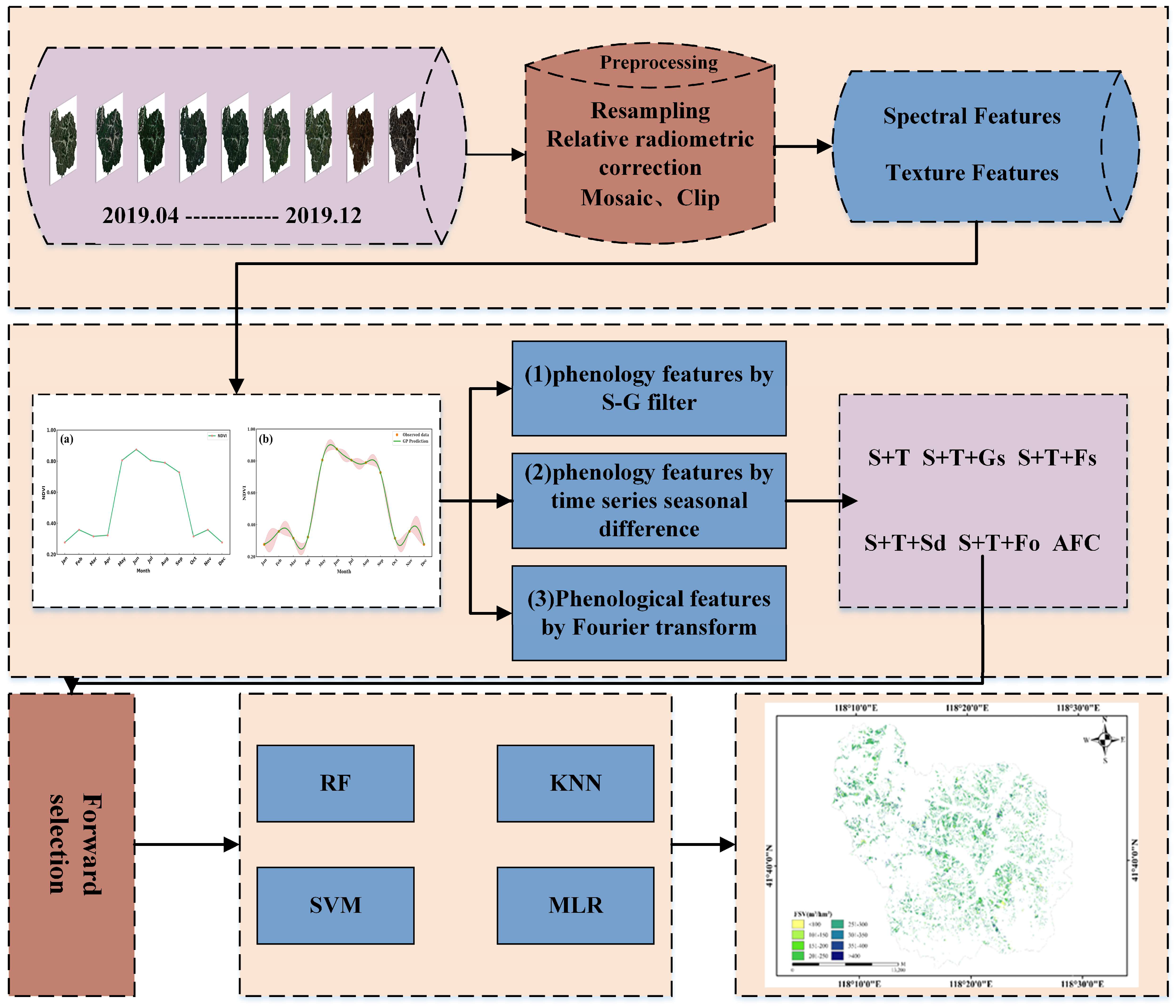
The remote sensing data in this study were acquired from the Sentinel-2 satellite, launched by the European Space Agency (ESA) in 2015. A total of nine Sentinel-2A L2A images from April to December 2019 was obtained from the Copernicus Open Access Hub (https://scihub.copernicus.eu/ accessed on 8 October 2023), excluding those affected by snow cover between January and March. These images underwent specific model processing techniques for acquisition purposes. Subsequently, all band data were resampled at a resolution of 20 m using SNAP 6.0 software for further analysis. Finally, these datasets were imported into Orfeo Toolbox (https://www.orfeo-toolbox.org/, accessed on 10 October 2023) to undergo a series of preprocessing steps including topographic correction and relative radiometric correction [25], ensuring accurate and reliable data for subsequent analysis. Additionally, all these data were divided into four seasons based on the growth characteristics of larch (Figure 3).

3. Research Methods

3.1. Spectral and Texture Feature Extraction

To accurately map FSV using Sentinel-2 images, it is crucial to extract valuable features through various methodologies. Typically, three types of features are considered, spectral features [26], vegetation indices, and texture features. In this study, 12 single-band information (including B1–B12) with a spatial resolution better than 20 m after resampling were selected as independent spectral features. Moreover, the vegetation index (VI) [14,15,16,17] was also employed as an indicator of surface vegetation cover and growth based on optical remote sensing data. After conducting comparative analysis and comprehensive assessment, this study opted for the selection of the top 15 vegetation indices (RVI, IPVI, NDVI, NDVI45, NDVI58a, NDVI56, GNDVI, IRECI, SAVI, ARV I, PSSRa, MTCI, MCARI, REIP and NDII) as key variables for mapping forest stock volume in subsequent modeling and research (

Table 1. Sentinel-2A List of Vegetation Index Characteristic Variables.

Variable Category	Variable Name	VI Calculation Formula
Vegetation index	Ratio Vegetation Index (RVI)	$RVI=\frac{B8}{B4}$
	Infrared Percentage Vegetation Index (IPVI)	$IPVI=\frac{B8}{(B8+B4)}$
	Normalized Difference Vegetation Index (NDVI)	$NDVI=\frac{(B8-B4)}{(B8+B4)}$
	Normalized Difference Vegetation Index 45 (NDVI45)	$NDVI45=\frac{(B5-B4)}{(B5+B4)}$
	Normalized Difference Vegetation Index 58a (NDVI58a)	$NDVI58a=\frac{(B8a-B5)}{(B8a+B5)}$
	Normalized Difference Vegetation Index 56 (NDVI56)	$NDVI56=\frac{(B6-B5)}{(B6+B5)}$
	Green Normalized Difference Vegetation Index (GNDVI)	$GNDVI=\frac{(B7-B3)}{(B7+B3)}$
	Inverted Red-Edge Chlorophyll Index (IRECI)	$IRECI=\frac{(B7-B4)}{(B5/B6)}$
	Soil-Adjusted Vegetation Index (SAVI)	$SAVI=1.5\times \frac{(B8-B4)}{8}\times (B8+B4+0.5)$
	Atmospherically Resistant Vegetation Index (ARVI)	$ARVI=\frac{(B8-(2\times B4-B2\left)\right)}{(B8+(2\times B4-B2\left)\right)}$
	Pigment-Specific Simple Ratio (PSSRa)	$PSSRa=\frac{B7}{B4}$
	Meris Terrestrial Chlorophyll Index (MTCI)	$MTCI=\frac{(B6-B5)}{(B5-B4)}$
	Modified Chlorophyll Absorption Ratio Index (MCARI)	$MCARI=\left(\right(B5-B4)-0.2\times (B5-B3\left)\right)\times (B5-B4)$
	Red Edge Inflection Point (REIP)	$REIP=700+40\times \frac{\left(\right(B4+B7)/2-B5)}{(B6-B5)}$
	Normalized Difference Infrared Index (NDII)	$NDII=\frac{B8-B11}{B8+B11}$

). Additionally, texture elements can provide crucial insights into forest density, tree species distribution, and growth status [14]. In this study, the grayscale co-production matrix method was employed to extract eight types of texture information from Sentinel-2A bands (Entropy, Contrast, Second moment, Homogeneity, Dissimilarity, Mean, Variance, and Correlation) [18], with a window size set at 5 × 5 [27,28,29].

3.2. Phenological Features Extracted from Time Series Sentinel-2 Images

3.2.1. Gaussian Process Regression to Reconstruct Time Series

Phenological features are typically derived from time series data in most cases. To mitigate observation errors, it is imperative to initially reconstruct the time series. The Gaussian Process Regression (GPR) algorithm is employed in this study to reconstruct the time series, and subsequently illustrate the extracted candidate information in Figure 4. A Gaussian process can be conceptualized as an ensemble of functions, where any set of function values (corresponding to any set of input values) follows a joint Gaussian distribution. Gaussian processes [30,31,32] are usually defined by the mean function $m\left(x\right)$ and the covariance function or kernel function $k(x,x^{\prime })$.

$$\mathit{f}\left(\mathit{x}\right)\sim \mathit{G}\mathit{P}\left(\mathit{m}\left(\mathit{x}\right),\mathit{k}\left(\mathit{x},{\mathit{x}}^{\prime }\right)\right)$$

(2)

where $m\left(x\right)$ is the mean value function, which represents the expected function value at a given point x. The kernel function $k(x,x^{\prime })$ represents the covariance of the function values between the two points x and x′.

Given a set of observation data points $D=\left\{\right(x1,y1),\dots ,(xn,yn\left)\right\}$, it is possible to predict the output value of the new point $x\ast$. In this study, due to the unavailability of remote sensing images from January to March, we employ a methodology that utilizes remote sensing data from October to December of the same year as a surrogate for estimating and supplementing the remote sensing features from March to January of the corresponding year. This approach acknowledges the presence of certain similarities and continuity in remote sensing features between adjacent months within the same geographical region.

3.2.2. Phenological Features

(1)

Extraction phenology features by S–G filter

Previous studies have demonstrated the significant potential of the Savitzky–Golay (S–G) filtering technique for accurately reconstructing time series data. Consequently, the S–G filter was used to smoothen the time series normalized vegetation index (NDVI) by fitting a low-order polynomial to a subset of selected data points [33,34,35] (Figure 5). Its expression is shown below:

$$y_i^{\prime }=\sum _{j=-m}^m{c}_j\cdot y_{i+j}$$

(3)

where ${\mathit{y}}_{\mathit{i}}^{\prime }$ is the filtered value, ${\mathit{y}}_{\mathit{i}+\mathit{j}}$ is the original data point, ${\mathit{c}}_{\mathit{j}}$ is the filter coefficient, and $\mathit{m}$ is the polynomial half the size of the window (the window size is $2m+1$).

In this study, a multi-temporal maximum value synthesis (MVC) method based on the S–G filtering algorithm was used to analyze the NDVI images of the current period. Subsequently, outliers were eliminated through a pixel-wise review of each image, and maximum values were determined by comparing them with the neighboring periods’ NDVI images. Interpolation methods were also utilized to recover data from rejected null image elements to enhance analysis accuracy. By analyzing the dynamics of the vegetation growth curves, botanical characteristics such as the start of the season (SOS), the end of the season (EOS), and the length of the season (LOS) [36] were extracted from key time nodes during the growing season (Figure 6). Furthermore, changes in vegetation indices and their textural features during the growing season of joint larch (April to September) could also serve as a phenological variable that reflects the growing season.

(2)

Extraction phenology features by time series seasonal difference

Given the deciduous nature of larch, its physiological and ecological features exhibit significant seasonal variations. In this study, the mean values of the feature variables were initially calculated within four seasons (spring: April and May; summer: June, July, and August; autumn: September and October; winter: November and December) to represent phenological features during spring, summer, autumn, and winter, respectively. Subsequently, a stepwise differencing method [37,38] was employed to differentiate the periodic data. The seasonally varying phenological features of larch were extracted by calculating the differences between features extracted from the current season and the previous season. Stepwise differencing is particularly useful for analyzing or predicting time series data or signals as it stabilizes non-stable time series data by eliminating trends and seasonal components. The detailed flow chart is shown in Figure 7.

(3)

Phenological features derived by Fourier transform

Time series spectral and textural information reconstructed by the Gaussian Process Regression (GPR) was transformed into the frequency domain using the Fourier transform algorithm [39,40,41], as illustrated in Figure 8, enabling the extraction of phenological indicators such as seasonal integrals and growing season amplitudes. The expression for the continuous-time Fourier transform is as follows:

$$X\left(f\right)={\int }_{-\mathrm{\infty }}^{\mathrm{\infty }}x\left(t\right)e^{-j2\pi ft}dt$$

(4)

where $X\left(f\right)$ is the Fourier transform of the signal $x\left(t\right)$, $f$ is the frequency, and $e^{-j2\pi ft}$ is the complex exponential function used to decompose the signal into sine and cosine waves. Assuming that the frequency range of NDVI index variation is $[f_1,f_2]$, the frequency components of the growing season by filtering $X\left(f\right)$ can be extracted as follows:

$$X_{\mathrm{growth}}\left(f\right)=\left\{\begin{array}{ll}X\left(f\right)& \mathrm{if} f_1\le f\le f_2\\ 0& \mathrm{otherwise} \end{array}\right.$$

(5)

$$A_{\mathrm{avg}, \mathrm{growth}}=\frac{1}{N_{\mathrm{growth} }}\sum _{k=1}^{N_{\mathrm{growth}}}{A}_{\mathrm{growth}}\left(k\right)$$

(6)

where $N_{\mathrm{growth}}$ is the number of valid frequencies for k, i.e., $f_2-f_1+1$.

3.3. Feature Selections

The mapping of forest stock volume is typically achieved by utilizing optimal feature sets extracted from remotely sensed data through feature selection methods [42,43,44]. Various feature selection methods have been widely applied to reduce model complexity and enhance prediction accuracy. In this study, the Forward Selection algorithm (Forward Selection) [45] was employed to select the optimal feature sets in combination with four regression models. To evaluate the capability of phenological features extracted from different methods, all alternative features were divided into six subsets, the subset of spectral and texture features (S + T), the subset of spectral, texture features, and growing season features (S + T + Gs), the subset of spectral, texture, and four-season features (S + T + Fs), the subset of spectral, texture, and seasonal difference features (S + T + Sd), and the subset of spectral, texture, and mean amplitude features fusion (S + T + Fo), and all features (AFC).

3.4. Modeling and Accuracy Evaluation

To demonstrate the applicability of various regression models for mapping FSV in Larch forests, the optimal feature sets were employed to construct the models. In this study, there are four models [46,47,48,49], including Multiple Linear Regression (MLR), Random Forest (RF), K-Nearest Neighbors (KNN), and Support Vector Machine (SVM). We utilized wrapper feature selection methods to construct regression models in R 4.2.0 software for mapping the FSV. In this approach, the K-Nearest Neighbors (KNN) model required the tuning of the number of neighbors (K). For the Random Forest (RF) model, the parameters to adjust included the number of trees (ntree) and the number of random variables required to split each node (mtry). The Support Vector Machine (SVM) model necessitated tuning the penalty coefficient (C) and gamma. The Multiple Linear Regression (MLR) model did not require parameter adjustments. Furthermore, the leave-one-out cross-validation (LOOCV) method was also employed to evaluate the accuracy of models. Three accuracy indices, including the coefficient of determination (R²), root mean square error (RMSE), relative root mean square error (rRMSE), were chosen to evaluate the performance of models. The aforementioned methods are summarized. Figure 9 illustrates the technical route for mapping forest stock volume using phenological feature data extraction.

$${\mathrm{R}}^2=1-\frac{\sum _{\mathrm{i}=1}^{\mathrm{n}}{\left({\mathrm{y}}_{\mathrm{i}}-{\widehat{\mathbf{y}}}_{\mathrm{i}}\right)}^2}{\sum _{\mathrm{i}=1}^{\mathrm{n}}{\left({\mathbf{y}}_{\mathrm{i}}-{\overline{\mathbf{y}}}_{\mathrm{i}}\right)}^2}$$

(7)

$$\mathrm{RMSE} =\sqrt{\frac{1}{n}\sum _{i=1}^n{\left(y_i-{\widehat{y}}_i\right)}^2}$$

(8)

$$\mathrm{rRMSE} =\left(\frac{ \mathrm{RMSE} }{\overline{\mathrm{y}}}\right)\times 100\mathrm{\%}$$

(9)

where $\widehat{\mathbf{y}}$ denotes the predicted FSV of samples, ${\mathrm{y}}_{\mathrm{i}}$ denotes the ground measured FSV of samples, $\overline{y}$ denotes the mean value of all samples, and n denotes the number of samples.

4. Results

4.1. Sensitivity between Features and FSV

In this study, all alternative features derived from time series Sentinel-2A images, encompassing spectral, texture, and phenological features, were classified into six groups for the purpose of mapping FSV. The sensitivity between these features and FSV was further examined through the absolute values of Pearson’s correlation coefficients. Figure 10a–f illustrate the top ten correlation coefficients between each feature group and FSV. Among these features, phenological features extracted from the growing season (Figure 10c) and seasonal differences (Figure 10e) exhibited strong correlations with FSV, as evidenced by their absolute values of Pearson’s correlation coefficients, ranging from 0.39 to 0.50 and 0.33 to 0.54, respectively. Conversely, traditional textural features demonstrated weaker correlations with FSV based on their absolute values of correlation coefficients ranging from 0.23 to 0.39. It is implied that phenological features display higher sensitivity with FSV than spectral and texture features.

4.2. Results of Estimated FSV without Phenological Features

The capability of phenological features was evaluated by initially deriving the estimated FSV using four models. These models utilized a subset of spectral and textural features extracted from Sentinel-2 images acquired between April and September, which corresponds to the larch growing season. The accuracy of the models was assessed using the coefficient of determination (R²), root mean square error (RMSE), and relative root mean square error (rRMSE), as shown in

Table 2. The accuracy indices of evaluating estimated FSV using spectral and textural features extracted from Sentinel-2 images acquired between April and September.

Acquird Date	Model	R2	RMSE (m3/hm2)	rRMSE (%)	Number of Features
April	RF	0.31	70.19	34.49	4
	KNN	0.41	63.46	31.18	9
	SVM	0.14	76.27	37.47	23
	MLR	0.38	65.05	31.96	9
May	RF	0.40	63.77	31.33	6
	KNN	0.51	57.73	28.37	11
	SVM	0.27	71.86	35.31	32
	MLR	0.49	58.91	28.95	9
June	RF	0.31	68.99	33.89	7
	KNN	0.51	57.73	28.36	12
	SVM	0.30	68.83	33.82	18
	MLR	0.48	59.73	29.35	8
July	RF	0.33	67.41	33.12	7
	KNN	0.52	56.78	27.89	17
	SVM	0.21	73.61	36.17	24
	MLR	0.46	60.79	29.87	9
August	RF	0.38	66.39	32.62	4
	KNN	0.48	60.02	29.49	13
	SVM	0.30	68.94	33.87	24
	MLR	0.48	59.24	29.11	8
September	RF	0.40	63.71	31.30	4
	KNN	0.52	56.76	27.89	12
	SVM	0.38	67.21	33.03	26
	MLR	0.50	58.68	28.83	9

. It is evident that the accuracy of the mapped FSV varied depending on the choice of model and acquisition date of images. The values for R² ranged from 0.14 to 0.52, while rRMSE ranged from 27.89% to 37.47%. Notably, the highest R² value and lowest rRMSE were achieved when KNN was employed with the images acquired in July and September, respectively. Furthermore, it was observed that the highest accuracy for mapped FSV was obtained from images acquired in September.

To further analyze the results of the estimated FSV, the optimal results (images acquired in September) were chosen to depict the scatter plots between the ground measured and predicted FSV (Figure 11). It is evident that overestimation occurred in young Larch forests, while underestimation was observed in mature ones. Even for samples with FSV ranging from 100 m³/hm² to 300 m³/hm², the accuracy of the results was significantly limited by errors arising from normal spectral and textural features. Therefore, it is imperative to incorporate new features to enhance estimation accuracy.

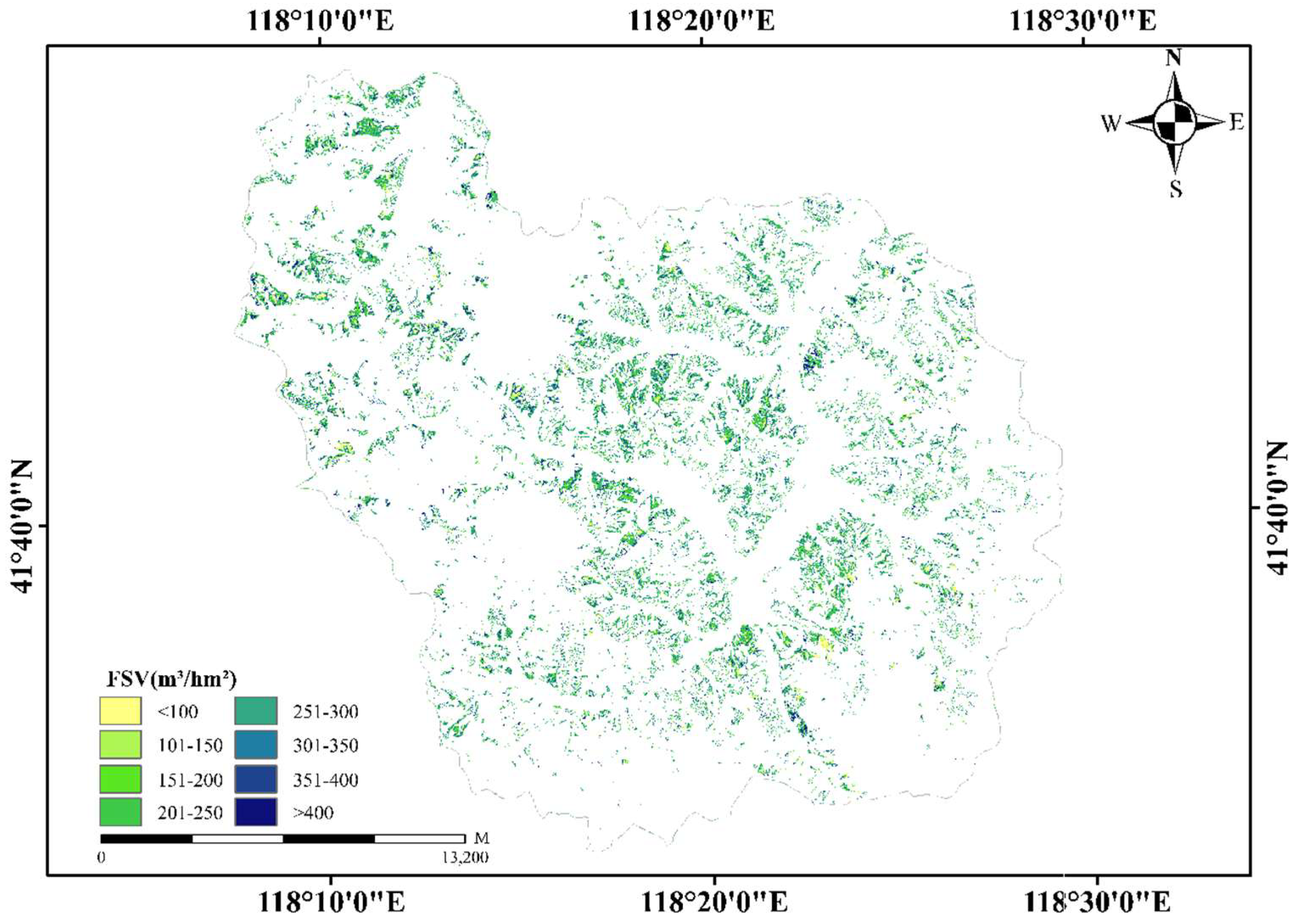
4.3. Results of Estimated FSV after Incorporating Phenological Features

In this study, further explorations were conducted to evaluate the potential of phenological features for mapping forest FSV in Larch forests. Spectral and textural features were extracted from the images acquired in September, while four types of phenological features were derived from time series images using various methods. Subsequently, six subsets (S + T, S + T + Gs, S + T + Fs, S + T + Sd, S + T + Fo, AFC) were obtained from an alternative feature set extracted from time series Sentinel-2A images using the Forward Selection algorithm coupled with four corresponding model regressors. A comprehensive overview of the results for each group can be found in

Table A1. Hierarchical feature variable filtering results.

Category	Model	Optimal Variable Eigenvalues
S + T	RF	PSSRa, NDVI58a, b11, b5.var
	KNN	NDVI56, b11, b2.var, b12.var, b3.var, MTCI, b11.Con, b5.Con, GNDVI, b12, b4.var, b12.Con
	SVM	b4, b12.Sec, b6.Con, b5.Cor, b7.Ent, RVI, b9.Ent, b6.Cor, b12.Cor, b4.Mea, b2.Sec, b8.Ent, b12, b1.Cor, b12.Ent, b8.var, b9.Hom, b4.Cor, b4.Sec, b9, b3.Sec, b1Ent, REIP, b8A.Cor, b3.Ent, b2.Ent
	MLR	b11, b3.Mea, b12.Ent, b6.var, b2.Mea, MTCI, b11.Cor, b2.Dis, b3.var
S + T + Gs	RF	PSSRa, b11.GSC4., NDVI56.GSC8., NDVI56, MTCI.GSC5., b3.var.GSC8., b2.Hom.SOS, b9.Con.EOS.
	KNN	NDVI56, b11, b4.GSC8., b11.GSC9., PSSRa, GNDVI.GSC7., b9.Con.GSC5., b2.GSC7., b4.GSC7., b2.Mea.GSC6., b2.var.GSC6., b2.Hom.GSC6., b2.Con.GSC6., b2.Dis.GSC6., b2.Ent.GSC6., b2.Sec.GSC6., b2.Cor.GSC6., b4.Mea.GSC6., b4.var.GSC6., b4.Cor.GSC6., b2.Mea.GSC5., b2.var.GSC5., b2.Hom.GSC5., b2.Con.GSC5., b2.Dis.GSC5., b2.Ent.GSC5., b2.Sec.GSC5., b2.Cor.GSC5., b8.Sec.SOS., NDVI56.SOS.,
	SVM	b5.Mea.GSC8., MTCI.GSC5., b3.Cor.GSC8., b4.Hom.GSC4., b3.var.GSC6., b3.Sec.GSC5., b8A.Ent.GSC7., b9.Hom.GSC8., b5.Cor, b3.Cor.GSC6., b1.Sec.GSC6., NDVI58a, b5.Cor.GSC8., b8A.Con.GSC7., b9.Ent.GSC4., b5.Hom.SOS., b8A.Ent.EOS.
	MLR	b11, b3.Mea, NDVI56.GSC4., b7.var.GSC5., b12.Sec.GSC8., b2.var, b5.Mea.GSC8., b11.Cor.GSC4., b9.var.GSC7., b4.Mea, b11.Sec.GSC4., b8A.Ent, b8A.Cor.GSC4., b3.Cor.GSC8., b11.Cor.GSC6., b5.Con.EOS., b8.Con.EOS., b3.var.EOS.,
S + T + Fs	RF	PSSRa, b11.Mea.Su., b11.Dis.Sp., b1mea.Wi., b4.Wi., b11.Cor.Sp., b1.Con.Sp.
	KNN	NDVI56, b11, b2.Con.Wi., b8A.Wi., b11.Au., b2.var.Wi., RVI.Wi., b2.var PSSRa.Wi., IRECI, b2.Con, b12.Sec, IPVI,
	SVM	b4, b1mea.Wi., MTCI.Sp., b11.Mea..Sp., b8.Ent, MCARI, b1.Cor.Su., b7.Ent, b4.Cor.Sp., b8.Hom.
	MLR	b11, b1mea.Wi., b12.Hom, b8ASec, b12.Au., b11.Mea.Au., b8.Hom.Wi., b12.Ent.Su., b6.Cor.Sp., b1Dis
S + T + Sd	RF	PSSRa, b4.1.2., b1mea.3.4., b8.Ent.1.2., b4, b8A.Ent.3.4., b4.Con.2.3., b8.2.3., b12.Cor.3.4., b1.Hom, b9.Hom.3.4.
	KNN	NDVI56, b11, b2.Con.3.4., b4.Con, b12.Con.3.4., b6Dis.1.2., NDVIII.3.4., b2.var.3.4., b11.var, b12.var.2.3., b3.var.3.4., b3.var, b12.var
	SVM	b4, b8.Ent.1.2., b1Ent, b9.Dis.3.4., b3.Sec.1.2., NDVI58a.3.4., b7.Cor.1.2., b8.Mea.3.4., b1.Cor.2.3., b1Ent.3.4., b8.Hom.2.3., b4.Dis.3.4., b2.Dis, b1Dis.2.3., NDVI.1.2., b7.Hom
	MLR	b1mea.3.4., b8.Ent.3.4., b11, b2.var, b12.Hom.3.4., b9.Ent.1.2., b2.Sec.2.3., b12.Mea.3.4., NDVI56, b9.Cor.1.2., b12.3.4., b4.Con.3.4., REIP.1.2., b1Ent.1.2., PSSRa.3.4.
S + T + Fo	RF	PSSRa, b11, b8.Sec.real., b8
	KNN	NDVI56, b11, b2.Con.real., b12.Con, b11.Con.real., b4.var, b3.var, b12, b12.var, b12.Mea, b2.Mea.real., b2.var.real., b7.Sec, b11.Mea, b12.Dis, ARVI, b2.var, b7.Con, b5.var
	SVM	b4, b12.Sec, b6.Con, b5.Cor, IRECI.real., PSSRa, b8.Sec.real., b9.Ent, b2.Mea.real., b11, NDVI58a, b4.Cor, b3.Sec, b3.Mea, b12.Ent, b4.Cor.real., b8A.Ent, b4.Sec, b2.Sec, b9.Hom, b6.Cor, b2.Cor, b1.Hom, SAVI, b9.Ent.real., b6.var
	MLR	b11, b2.Mea.real., b12.Hom, b8A.Ent, b12.real., b11.Mea.real., b4.real., b5, b11.Cor.real., b8A.Con.real., b5.Cor.real., b4.Ent, b8.Ent
AFC	RF	PSSRa, b4.1.2., b1mea.Wi., b6.Con.1.2., b8A.Ent.3.4., b2.Sec.2.3., b8(real), NDVI(real)
	KNN	b11, b2.Con.3.4., SAVI.Wi., RVI.Wi., b2.Con.real., b11.Con.3.4., b11.Su., b9.var.2.3., PSSRa.Wi., b4.Mea.Su., b12.Au., b3.var.Su., IRECI.SOS., IRECI.Wi., b12.Con, b12.Sp., ARVI.Au., NDVI58a.Au., RVI.SOS., NDVI56.EOS., b4.var
	SVM	ARVI, b2.Hom.EOS., b9.Cor.Wi., b8A.Ent.3.4., b3.Mea.3.4., b3.Cor.real., NDVIII.3.4., NDVI56.2.3., b1.Cor, b5.var.2.3., b8.Sec.SOS., b4.Cor.2.3., b2.Cor.real., b4, b12.Sec.3.4., PSSRa.3.4., b11.Con..Sp., b7.Sec, b1Ent.1.2., b1.Cor.real., b9.Sec.3.4.
	MLR	b1mea.3.4., b8.Ent.3.4., b4.SOS., b3.Mea.EOS., b9.Ent.1.2., b8.Mea.real., REIP.3.4., b8.var.1.2., b5.Dis.3.4., RVI.Sp., b4.Mea.3.4., b8A.Ent.2.3., b9.Hom, b9.Sec.EOS., b2.Hom.3.4., b3.Hom, b4.Ent.Au. b2.1.2., b4.Hom.Su., b6.Sec.3.4.

. These selected feature subsets were then utilized to map FSV using four models and the outcomes are presented in

Table 3. The accuracy indices of evaluating estimated FSV after incorporating phenological features.

Subsets of Features	RF		KNN		SVM		MLR
	R2	rRMSE (%)	R2	rRMSE (%)	R2	rRMSE (%)	R2	rRMSE (%)
S + T	0.40	31.30	0.52	27.89	0.38	33.03	0.50	28.83
S + T + Gs	0.47	30.16	0.57	26.60	0.55	28.11	0.58	26.16
S + T + Fs	0.54	29.33	0.67	23.29	0.48	29.64	0.64	24.34
S + T + Sd	0.58	28.03	0.65	24.05	0.39	31.97	0.63	24.34
S + T + Fo	0.41	31.14	0.61	25.11	0.44	31.77	0.61	25.02
AFC	0.59	28.12	0.68	22.95	0.77	22.78	0.67	23.15

.

The results indicate a significant improvement in the accuracy of mapped forest stock volume (FSV) after incorporating various phenological features. Specifically, when compared to subset 1 (S + T), subsets 2 to 5 showed determination coefficients (R²) ranging from 0.38 to 0.77 and relative root mean square error (rRMSE) ranging from 22.78% to 33.03%. This suggests that phenological features have greater potential for capturing changes in forest structure parameters compared to normal spectral and textural features, particularly for Larch forests. Notably, optimal training performance was achieved by including all types of phenological features (AFC) using SVM regressor, resulting in an R² value of 0.77 and an rRMSE value of 22.78%. Therefore, incorporating phenological features can improve the accuracy and reliability of mapping FSV, with the degree of improvement closely associated with methods of extracting phenological features. To further explore the response of different feature factors to FSV, scatter plots were generated between predicted and measured FSV for the model with the highest estimation accuracy (Figure 12). Furthermore, it is demonstrated that phenological features hold great potential for improving the accuracy of mapping FSV in Larch forests, resulting in reduced discrepancies between ground measured and predicted FSV values. It is further proven that by incorporating diverse phenological features, the accuracy of FSV estimation can be significantly enhanced, particularly in terms of mitigating underestimation errors.

Based on the accuracy of results (Table 3), the map of FSV in planted Larch forests was generated by Optimal model SVM using spectral and textural features extracted from images acquired in September and four types of phenological features (Figure 13). Within our study area, plantation forests primarily displayed a concentration of FSV ranging from 100 to 300 m³/hm², accounting for over 25.28% of the total coniferous plantation area. Specifically, the average volume of coniferous larch within this region was calculated as 208.36 m³/hm², with a standard deviation of 33.58 m³/hm².

5. Discussion

5.1. Sensitivity Analyses of Phenological Features and FSV

Numerous studies have demonstrated that larch leaves undergo significant phenological changes throughout the annual cycle, reflecting their adaptability to shifts in phenology [2,3]. Specifically, from January to March, larches enter a dormant phase characterized by the absence of leaf growth, marking the non-growing season [36]. Subsequently, from April to September, larches transition into the leaf growth phase with a rapid development of leaves, showcasing their robust growth vitality. By October, the trees initiate the leaf senescence phase as leaves exhibit signs of aging and yellowing, indicating the onset of autumn. Finally, from November to December, larches re-enter a dormant state. Therefore, larches can be considered as one of the key species for studying phenological changes.

Previous research suggests that the phenological features reflect the forest’s responses to environmental changes and can serve as indicators for assessing the health and productivity of forest [4]. Therefore, this study aimed to explore the sensitivity between phenological features and FSV in a planted larch forest. Initially, nine Sentinel-2A remote sensing images were acquired, and textural and spectral features were extracted for each scene. After that, features were subsequently smoothed and reconstructed using the Gaussian Process Regression (GPR) algorithm. Subsequently, the phenological features were extracted from time series images using four methods, such as the Savitzky–Golay filter, stepwise differencing, and Fourier Transform. Additionally, Pearson’s correlation analysis was conducted on the spectral variables, vegetation indices, texture features, and phenological features. The results revealed that compared to traditional spectral and textural variables, all phenological features extracted through various methods exhibited significant correlations. Among these features, phenological features extracted from growing season characteristics and seasonal change patterns demonstrated higher sensitivity levels (0.39~0.50). Furthermore, during the process of feature selection using the forward selection method, phenological features also exhibited a substantial contribution within the optimal feature set, thereby further substantiating their significance in estimating forest stock volume.

Existing research has unveiled that the introduction of phenological features brings a new perspective to the domain of forest resource monitoring. Phenological features have demonstrated high sensitivity and practical value in applications such as forest landform identification, monitoring the dynamics of plant communities, assessing the impacts of drought or pestilence, and forecasting the aboveground biomass of forests [50,51,52]. Moreover, this study has transcended the approach of extracting phenological features through a single method by employing a variety of techniques, including Savitzky–Golay filters, stepwise differencing, and Fourier transforms. This approach allows for the layered extraction of phenological features from multiple datasets, thereby achieving high precision in the extraction of phenological features. Additionally, the Gaussian Process Regression (GPR) algorithm has effectively addressed the noise issues encountered in the extraction of phenological features in large-scale spatial applications.

In comparison to previous studies, this research provides additional evidence supporting the efficacy of phenological features as functional indicators for assessing forest ecosystem and its associated stock volume.

5.2. Contribution of Phenological Features in Mapping FSV

The impact of phenological features on the timing and efficiency of plant growth activities indirectly regulates the growth rate of forest. Previous studies have demonstrated that these features closely associated with forest stock volume can effectively reduce the errors caused by underestimation and delay saturation issues, thereby significantly enhancing the precision of mapping FSV [53,54]. In this study, phenological features from Sentinel-2A data were incorporated into the regression model in a planted larch forest, and the results demonstrated that including various phenological features can improve the accuracy of mapping FSV to a certain extent. In particular, integrating all the phenological features yielded the optimal estimation accuracy (R² = 0.77, rRMSE = 22.78%). The inclusion of various phenological features resulted in a significant improvement in the determination coefficient (R²), with an increase of 0.25. Additionally, the root mean square error (RMSE) was reduced by 10.40 m³/hm² and the relative root mean square error (rRMSE) decreased by approximately 5% when compared to traditional spectral and textural variables (Figure 14).

Furthermore, previous results have proven that the improvement of accuracy in mapping FSV is attributed to the incorporation of novel features, thereby mitigating the underestimation of predicted FSV [55]. Scholars have confirmed that incorporating structural features (such as tree height and stand density) and topographical features (such as slope and aspect), as well as climatic characteristics (including long-term climate data like temperature and precipitation) on the basis of spectral and textural variables, can significantly reduce the underestimation of forest stock volume predictions, thereby enhancing the accuracy of the prediction models. This study also demonstrates significant effectiveness in reducing the underestimation of forest stock volume and improving the estimation accuracy by adding phenological features that reflect the seasonal changes in vegetation growth on the basis of spectral and texture variables. Furthermore, studies have shown that phenological features are highly effective in forest land object identification, monitoring plant community growth dynamics, assessing the impacts of drought or pests, and predicting forest aboveground biomass [50,51,52].

This further emphasizes the importance of employing a comprehensive range of phenological features in forest resource estimation while providing novel perspectives and theoretical foundations for future forest resource management and assessment.

6. Conclusions

To accurately map the forest stock volume of northern larch plantations, this study extracted spectral features, texture features, and phenological features from the Sentinel-2A time series data set. Optimal variables from each variable set were selected in conjunction with Pearson’s correlation coefficients and forward feature selection methods; thereafter, four machine learning models were constructed—Multiple Linear Regression (MLR), K-Nearest Neighbors (KNN), Random Forest (RF), and Support Vector Machine (SVM). The results indicate that phenological variables demonstrate a higher sensitivity towards the forest volume of larch compared to spectral and textural variables, with Pearson’s correlation coefficient reaching an absolute value of 0.54. Incorporating phenological variables into the forest volume estimation model significantly improved accuracy (R² increased by 0.25, RMSE decreased by 10.40 m³/hm², and rRMSE decreased by 5%), thereby mitigating the underestimation of samples with larger accumulations. These findings suggest that phenological features extracted from Sentinel-2A time series data hold significant potential for enhancing forest stock estimation. Future studies will further explore the application of phenological features in estimating forest stock for other tree species while optimizing their extraction methods to more accurately reflect the forest stock of each specific tree species.

References

1. Leng, W.; He, H.S.; Bu, R.; Dai, L.; Hu, Y.; Wang, X. Predicting the distributions of suitable habitat for three larch species under climate warming in Northeastern China. For. Ecol. Manag. 2008, 254, 420–428. [Google Scholar] [CrossRef]
2. Duan, B.; Xiao, R.; Cai, T.; Man, X.; Ge, Z.; Gao, M.; Mencuccini, M. Strong Responses of Soil Greenhouse Gas Fluxes to Litter Manipulation in a Boreal Larch Forest Northeastern China. Forests 2022, 13, 1985. [Google Scholar] [CrossRef]
3. Yu, Z.; Man, X.; Cai, T.; Shang, Y. How Potential Evapotranspiration Regulates the Response of Canopy Transpiration to Soil Moisture and Leaf Area Index of the Boreal Larch Forest in China. Forests 2022, 13, 571. [Google Scholar] [CrossRef]
4. Fu, W.; Li, L.; Luo, M.; Chen, J.; Wang, F. Spillover Effect of Forest Carbon Sinks and Influencing Factors from a Provincial Perspective in China. Acta Ecol. Sin. 2023, 43, 4074–4085. [Google Scholar]
5. Amini, M.; Habashi, H.; Amini, R. A survey on the accuracy of the inventory method of sample plots with 1000m2 area under randomsystematic network for estimation of amount and distribution of stand volume basal area and tree number in diameter classes. Iran. J. For. Poplar Res. 2007, 15, 195–206. [Google Scholar]
6. Liu, Z.; Ye, Z.; Xu, X.; Lin, H.; Zhang, T.; Long, J. Mapping Forest Stock Volume Based on Growth Characteristics of Crown Using Multi-Temporal Landsat 8 OLI and ZY-3 Stereo Images in Planted Eucalyptus Forest. Remote Sens. 2022, 14, 5082. [Google Scholar] [CrossRef]
7. Xu, X.; Li, H.; Liu, Z.; Ye, Z.; Lin, X.; Long, J. A Combined Strategy of Improved Variable Selection and Ensemble Algorithm to Map the Growing Stem Volume of Planted Coniferous Forest. Remote Sens. 2021, 13, 4631. [Google Scholar] [CrossRef]
8. David, R.M.; Rosser, N.J.; Donoghue, D.N.M. Improving above ground biomass estimates of Southern Africa dryland forests by combining Sentinel-1 SAR and Sentinel-2 multispectral imagery. Remote Sens. Environ. 2022, 282, 113232. [Google Scholar] [CrossRef]
9. Yang, X.; Qiu, S.; Zhu, Z.; Rittenhouse, C.D.; Riordan, D.P.; Cullerton, M. Mapping understory plant communities in deciduous forests from Sentinel-2 time series. Remote Sens. Environ. 2023, 293, 113601. [Google Scholar] [CrossRef]
10. Quang, A.V.; Delbart, N.; Jaffrain, G.; Pinet, C.; Moiret, A. Detection of degraded forests in Guinea, West Africa, based on Sentinel-2 time series by inclusion of moisture-related spectral indices and neighbourhood effect. Remote Sens. Environ. 2022, 281, 113230. [Google Scholar] [CrossRef]
11. Silvetti, L.E.; Marisa, B. Detection of woody species Schinopsis haenkeana using phenological spectral differences and NDVI texture measures in subtropical forests. Remote Sens. Appl. Soc. Environ. 2024, 33, 101128. [Google Scholar] [CrossRef]
12. Vorovenci, I.I.; Dincă, L.; Crișan, V.; Postolache, R.G.; Coșofreț, V.R.; Leonid, C.; Cristian, C.; Grecjiță, C.I.; Chima, S. Local-scale mapping of tree species in a lower mountain area using Sentinel-1 and -2 multitemporal images, vegetation indices, and topographic information. Front. For. Glob. Chang. 2023, 6, 1220253. [Google Scholar] [CrossRef]
13. Ma, T.; Hu, M.; Wang, H.; Beckline, M.; Pang, D.; Chen, L.; Ni, X.; Li, X. A Novel Vegetation Index Approach Using Sentinel-2 Data and Random Forest Algorithm for Estimating Forest Stock Volume in the Helan Mountains, Ningxia, China. Remote Sens. 2023, 15, 1853. [Google Scholar] [CrossRef]
14. Abdollahnejad, A.; Panagiotidis, D. Tree Species Classification and Health Status Assessment for a Mixed Broadleaf-Conifer Forest with UAS Multispectral Imaging. Remote Sens. 2020, 12, 3722. [Google Scholar] [CrossRef]
15. Park, C.E.; Jeong, S.J. Land Surface Temperature Sensitivity to Changes in Vegetation Phenology Over Northern Deciduous Forests. J. Geophys. Res. Biogeosci. 2023, 128, e2023JG007498. [Google Scholar] [CrossRef]
16. Zheng, W.; Liu, Y.; Yang, X.; Fan, W. Spatiotemporal Variations of Forest Vegetation Phenology and Its Response to Climate Change in Northeast China. Remote Sens. 2022, 14, 2909. [Google Scholar] [CrossRef]
17. Li, F.; Song, G.; Liu, Z.; Zhou, Y.; Lu, D. Urban vegetation phenology analysis using high spatio-temporal NDVI time series. Urban For. Urban Green. 2017, 25, 43–57. [Google Scholar] [CrossRef]
18. Yan, W.; Yang, F.; Zhou, J.; Wu, R. Droughts force temporal change and spatial migration of vegetation phenology in the northern Hemisphere. Agric. For. Meteorol. 2023, 341, 109685. [Google Scholar] [CrossRef]
19. Zhang, Y.; Li, M. A new method for monitoring start of season (SOS) of forest based on multisource remote sensing. Int. J. Appl. Earth Obs. Geoinf. 2021, 104, 102556. [Google Scholar] [CrossRef]
20. Li, H.; Yan, E.; Jiang, J.; Mo, D. Monitoring of key Camellia Oleifera phenology features using field cameras and deep learning. Comput. Electron. Agric. 2024, 219, 108748. [Google Scholar] [CrossRef]
21. Guan, P.; Zheng, Y.; Lei, G.; Liu, Y.; Zhu, L.; Guo, Y.; Wang, Y.; Xi, B. Near-Earth Remote Sensing Images Used to Determine the Phenological Characteristics of the Canopy of Populus tomentosa B301 under Three Methods of Irrigation. Remote Sens. 2022, 14, 2844. [Google Scholar] [CrossRef]
22. Yi, L.; Shu-Hua, G.; Zhong-Liu, J.; Wen-Jun, L.; Kai-Long, H.; Jia-Yi, Z.; Yu-Hui, O.; Ying, L. Phenological characteristics of airborne pollen and its relationship with meteorological factors in Haidian District, Beijing, China during the period of 2012–2016. Ji Ying Yong Sheng Tai Xue Bao/J. Appl. Ecol. 2019, 30, 3563–3571. [Google Scholar]
23. Zheng, H.; Long, J.; Zang, Z.; Lin, H.; Liu, Z.; Zhang, T.; Yang, P. Interpreting the Response of Forest Stock Volume with Dual Polarization SAR Images in Boreal Coniferous Planted Forest in the Non-Growing Season. Forests 2023, 14, 1700. [Google Scholar] [CrossRef]
24. Jiang, F.; Kutia, M.; Ma, K.; Chen, S.; Long, J.; Sun, H. Estimating the aboveground biomass of coniferous forest in Northeast China using spectral variables, land surface temperature and soil moisture. Sci. Total Environ. 2021, 785, 147335. [Google Scholar] [CrossRef] [PubMed]
25. Moghimi, A.; Celik, T.; Mohammadzadeh, A. Tensor-based keypoint detection and switching regression model for relative radiometric normalization of bitemporal multispectral images. Int. J. Remote Sens. 2022, 43, 3927–3956. [Google Scholar] [CrossRef]
26. Ninomiya, Y.; Fu, B. Thermal infrared multispectral remote sensing of lithology and mineralogy based on spectral properties of materials. Ore Geol. Rev. 2019, 108, 54–72. [Google Scholar] [CrossRef]
27. Hashjin, S.S.; Khazaei, S.; Sadeghi, A. A Method to Select Coherence Window Size for forest height estimation using PolInSAR Data. Int. Arch. Photogramm. Remote Sens. Spat. Inf. Sci. 2013, XL-1/W3, 505–508. [Google Scholar] [CrossRef]
28. Qiu, Y.; Ming, D. Lithostratigraphic Classification Method Combining Optimal Texture Window Size Selection and Test Sample Purification Using Landsat 8 OLI Data. Open Geosci. 2018, 10, 565–581. [Google Scholar] [CrossRef]
29. Ratha, D.; Mandal, D.; Kumar, V.; McNairn, H.; Bhattacharya, A.; Ferreyro, A.C. A Generalized Volume Scattering Model-Based Vegetation Index from Polarimetric SAR Data. IEEE Geosci. Remote Sens. Lett. 2019, 16, 1795–1799. [Google Scholar] [CrossRef]
30. Ballabio, C.; Lugato, E.; Fernández-Ugalde, O.; Orgiazzi, A.; Jones, A.; Borrelli, P.; Montanarella, L.; Panagos, P. Mapping LUCAS topsoil chemical properties at European scale using Gaussian process regression. Geoderma 2019, 355, 113912. [Google Scholar] [CrossRef]
31. Bao, B.; Jin, S.; Li, L.; Duan, K.; Gong, X. Analysis of Green Total Factor Productivity of Grain and Its Dynamic Distribution: Evidence from Poyang Lake Basin, China. Agriculture 2022, 12, 8. [Google Scholar] [CrossRef]
32. De Caro, D.; Ippolito, M.; Cannarozzo, M.; Provenzano, G.; Ciraolo, G. Assessing the performance of the Gaussian Process Regression algorithm to fill gaps in the time-series of daily actual evapotranspiration of different crops in temperate and continental zones using ground and remotely sensed data. Agric. Water Manag. 2023, 290, 108596. [Google Scholar] [CrossRef]
33. Cao, R.; Chen, Y.; Shen, M.; Zhou, C.; Wang, C.; Yang, W. A simple method to improve the quality of NDVI time-series data by integrating spatiotemporal information with the Savitzky-Golay filter. Remote Sens. Environ. 2018, 217, 244–257. [Google Scholar] [CrossRef]
34. Peng, Y.; Qiao, Z.; Dong, Z.; Zhao, Y.; Zhou, X.; Wu, B.; Lin, Q. Noise Processing of Ocean Absolute Gravity Data Based on Savitzky-Golay Filtering Algorithm. J. Phys. Conf. Ser. 2023, 2651, 012154. [Google Scholar]
35. Wu, L.; Tang, W. The Optimum Time Window for Spartina Alterniflora Classification based on the Filtering Algorithm and Vegetation Phonology Using GEE. J. Geo-Inf. Sci. 2023, 25, 636–646. [Google Scholar]
36. Tyutkova, E.A.; Loskutov, S.R.; Shestakov, N.P. FTIR spectroscopy of early and latewood of Larix gmelinii growing along the polar treeline: The correlation between absorption bands and climatic factors. Wood Mater. Sci. Eng. 2019, 15, 205–212. [Google Scholar] [CrossRef]
37. Chen, L.; Han, J.; Fu, L.-Y.; Peng, W.; Song, C. A Compact High-Order Finite-Difference Method with Optimized Coefficients for 2D Acoustic Wave Equation. Remote Sens. 2023, 15, 604. [Google Scholar] [CrossRef]
38. Yan, H.; Liu, Y.; Zhang, H. Prestack reverse-time migration with a time-space domain adaptive high-order staggered-grid finite-difference method. Explor. Geophys. 2018, 44, 77–86. [Google Scholar] [CrossRef]
39. Li, X.; Liu, M.; Ma, H.; Wei, M.; Dai, Z. Hyperfine structure and isotope shift of neutral and singly ionized copper using Fourier transform spectroscopy. Results Phys. 2024, 57, 103721. [Google Scholar] [CrossRef]
40. Zhang, L.; Fu, L.; Pan, G.; Zhang, W.; Ren, G.; Zheng, Z.; Yang, Y. Elucidating the Multi-Timescale Variability of a Canopy Urban Heat Island by Using the Short-Time Fourier Transform. Geophys. Res. Lett. 2024, 51, e2023GL106221. [Google Scholar] [CrossRef]
41. Miao, C.; Ran, X.; Dai, K.; Wan, J.; Li, T.; Xu, W.; Yan, W.; Li, T.; Tong, K. Fine Classification Method for Massive Microseismic Signals Based on Short-Time Fourier Transform and Deep Learning. Remote Sens. 2023, 15, 502. [Google Scholar] [CrossRef]
42. Wang, X.; Zhang, C.; Qiang, Z.; Xu, W.; Fan, J. A New Forest Growing Stock Volume Estimation Model Based on AdaBoost and Random Forest Model. Forests 2024, 15, 260. [Google Scholar] [CrossRef]
43. Kumar, A.; Noliya, A.; Makani, R. Fuzzy inference based feature selection and optimized deep learning for Advanced Persistent Threat attack detection. Int. J. Adapt. Control Signal Process. 2023, 38, 604–620. [Google Scholar] [CrossRef]
44. Thakkar, A.; Kikani, N.; Geddam, R. Fusion of linear and non-linear dimensionality reduction techniques for feature reduction in LSTM-based Intrusion Detection System. Appl. Soft. Comput. 2024, 154, 111378. [Google Scholar] [CrossRef]
45. Hui, F.K.C.; Müller, S.; Welsh, A.H. GEE-Assisted Variable Selection for Latent Variable Models with Multivariate Binary Data. J. Am. Stat. Assoc. 2023, 118, 1252–1263. [Google Scholar] [CrossRef]
46. Pelletier, F.; Cardille, J.A.; Wulder, M.A.; White, J.C.; Hermosilla, T. Inter- and intra-year forest change detection and monitoring of aboveground biomass dynamics using Sentinel-2 and Landsat. Remote Sens. Environ. 2023, 301, 113931. [Google Scholar] [CrossRef]
47. Fan, D. Research on the establishment of NDVI long-term data set based on a novel method. Sci. Rep. 2023, 13, 9838. [Google Scholar] [CrossRef] [PubMed]
48. Thapa, B.; Lovell, S.; Wilson, J. Remote sensing and machine learning applications for aboveground biomass estimation in agroforestry systems: A review. Agrofor. Syst. 2023, 97, 1097–1111. [Google Scholar] [CrossRef]
49. Mondal, P.; Shukla, S.; McDermid, S.; Qadir, A. A reporting framework for Sustainable Development Goal 15: Multi-scale monitoring of forest degradation using MODIS, Landsat and Sentinel data. Remote Sens. Environ. 2020, 237, 111592. [Google Scholar] [CrossRef]
50. Sun, H.; Wang, B.; Wu, Y.; Yang, H. Deep Learning Method Based on Spectral Characteristic Rein-Forcement for the Extraction of Winter Wheat Planting Area in Complex Agricultural Landscapes. Remote Sens. 2023, 15, 1301. [Google Scholar] [CrossRef]
51. Ponomarev, V.I.; Klobukov, G.I.; Napalkova, V.V.; Akhanaev, Y.B.; Pavlushin, S.V.; Yakimova, M.E.; Subbotina, A.O.; Picq, S.; Cusson, M.; Martemyanov, V.V. Phenological Features of the Spongy Moth, Lymantria dispar (L.) (Lepidoptera: Erebidae), in the Northernmost Portions of Its Eurasian Range. Insects 2023, 14, 276. [Google Scholar] [CrossRef] [PubMed]
52. Zhang, X.; Shen, H.; Huang, T.; Wu, Y.; Guo, B.; Liu, Z.; Luo, H.; Tang, J.; Zhou, H.; Wang, L.; et al. Improved random forest algorithms for increasing the accuracy of forest aboveground biomass estimation using Sentinel-2 imagery. Ecol. Indic. 2024, 159, 111752. [Google Scholar] [CrossRef]
53. Chen, Z.; Zhang, M.; Zhang, H.; Liu, Y. Mapping Mangrove Using a Red-Edge Mangrove Index (REMI) Based on Sentinel-2 Multispectral Images. IEEE Trans. Geosci. Remote Sens. 2023, 61, 4409511. [Google Scholar] [CrossRef]
54. Arne, N.; Christoph, G.; Ralf, K.B.; Gernot, R.; Tim, R.; Karl, S.; Andrew, O.F. Estimating Timber Volume Loss due to Storm Damage in Carinthia, Austria, using ALS/TLS and Spatial Regression Models. For. Ecol. Manag. 2021, 502, 117914. [Google Scholar]
55. Liu, J.; Quan, Y.; Wang, B.; Shi, L.; Lang, M.; Li, M. Estimation of Forest Stock Volume Combining Airborne LiDAR Sampling Approaches with Multi-Sensor Imagery. Forests 2023, 14, 2453. [Google Scholar] [CrossRef]
Figure 1. The location of the study area and maps of ground samples: (a) is a map of the location of Inner Mongolia in China; (b) is a map of the location of the forest farm in Chifeng City; (c) is a sample point on the ground in the study area; (d,e) is a close-up photograph of a larch plantation forest.
Forests 15 00995 g001
Figure 2. The relationships among DBH, Height and FSV: (a) is the scatterplot of FSV and DBH; (b) is the scatterplot of FSV and Height.
Forests 15 00995 g002
Figure 3. Sentinel-2 images for four seasons.
Forests 15 00995 g003
Figure 4. Gaussian Process Regression to reconstruct NDVI: (a) Unreconstructed NDVI values; (b) Reconstructed NDVI values.
Forests 15 00995 g004
Figure 5. Schematic diagram of time series data reconstructed by S–G filter.
Forests 15 00995 g005
Figure 6. S–G filtering to reconstruct NDVI and extract phenology features.
Forests 15 00995 g006
Figure 7. Extracting phenological features using time series seasonal differences.
Forests 15 00995 g007
Figure 8. Fourier extraction of growing season amplitude variables.
Forests 15 00995 g008
Figure 9. The technical roadmap for mapping forest stock volume based on phenological feature data extraction.
Forests 15 00995 g009
Figure 10. Distribution of Pearson’s correlation coefficients between different types of features and FSV: (a) Spectral features; (b) Textural features; (cf) Phenological features by various methods.
Forests 15 00995 g010
Figure 11. The scatterplots between measured and predicted FSV using Sentinel-2A images acquired in September.
Forests 15 00995 g011
Figure 12. The scatterplots between the measured and predicted FSV using various phenological features.
Forests 15 00995 g012
Figure 13. The map of FSV in the planted larch forest of study area.
Forests 15 00995 g013
Figure 14. The histograms of accuracy indices derived from various subsets (a) the histograms of R2 derived from various subsets; (b) the histograms of rRMSE derived from various subsets.
Forests 15 00995 g014