Does Soil Acidification Matter? Nutrient Sustainability of Timber Harvesting in Forests on Selected Soils Developed in Sediments of the Early vs. Late Pleistocene

Zimmermann, Stephan; Kurz, Daniel; Thrippleton, Timothy; Mey, Reinhard; Perry, Niál Thomas; Posch, Maximilian; Schweier, Janine

doi:10.3390/f15071079

Open AccessArticle

Does Soil Acidification Matter? Nutrient Sustainability of Timber Harvesting in Forests on Selected Soils Developed in Sediments of the Early vs. Late Pleistocene

by

Stephan Zimmermann

^1,*

,

Daniel Kurz

²,

Timothy Thrippleton

¹,

Reinhard Mey

³

,

Niál Thomas Perry

¹,

Maximilian Posch

⁴ and

Janine Schweier

¹

Swiss Federal Institute for Forest, Snow and Landscape Research, 8903 Birmensdorf, Switzerland

²

EKG Geo-Science, 3011 Bern, Switzerland

³

Forestry Research and Competence Centre, ThüringenForst AöR, Jägerstr. 1, 99867 Gotha, Germany

⁴

International Institute for Applied Systems Analysis (IIASA), A-2361 Laxenburg, Austria

^*

Author to whom correspondence should be addressed.

Forests 2024, 15(7), 1079; https://doi.org/10.3390/f15071079

Submission received: 29 April 2024 / Revised: 11 June 2024 / Accepted: 15 June 2024 / Published: 21 June 2024

(This article belongs to the Special Issue The Influence of Forest Operations on the Sustainable Management of Forest Soils)

Download

Browse Figures

Review Reports Versions Notes

Abstract

:

With this study, our aim was to estimate the nutrient fluxes relevant for assessing nutrient sustainability as accurately as possible and to calculate nutrient balances for alternative forest management scenarios. Furthermore, we tested whether mapping units from existing geologic maps can serve as a basis for forest practitioners to estimate nutrient sustainability or whether more detailed data are needed. Positive fluxes include deposition and weathering, while negative fluxes include losses due to leaching and nutrient removal through timber harvesting in the balance. Weathering and leachate losses were modeled with a geochemical model. The SwissStandSim model was used to simulate the biomass growth under different harvesting and silvicultural strategies, allowing for sustainability to be assessed for each nutrient at a given intensity of use. This assessment was made per rotation period based on two criteria: (i) nutrient supply and (ii) total stocking volume. As a result, it can be noted that the accurate estimation of individual fluxes is essential for assessing the sustainability of forestry practices and that it needs detailed site-specific data. Various influencing factors turned out to be important, particularly the assumed depth of the root zone.

Keywords:

wood nutrient contents; whole-tree harvest; stem wood harvest; nutrient sustainability; nutrient mass balances; base cations; nitrogen; phosphorus

Graphical Abstract

1. Introduction

In view of climate change, efforts are being made to replace fossil fuels with renewable energy sources. Wood is a naturally renewable raw material that can be climate-neutral when used sustainably as an energy resource. Wood biomass is also available regardless of seasonal fluctuations. Due to these facts, the use of energy wood has been intensified in recent years, especially on the Swiss Plateau, and in some cases the aim is to harvest as much of the above-ground tree biomass as possible (whole-tree harvesting). This has, however, more profound consequences on the forest ecosystem than the removal of stemwood. Due to its effect on forest nutrient cycling [1] as well as on biodiversity [2,3], it is therefore controversially discussed. As a large proportion of nutrients are stored in needles/leaves, twigs, and bark, the removal of nutrients is significantly increased by whole-tree harvesting [4,5,6,7].

Particularly on acidified, nutrient-poor sites, this can lead to problems in terms of nutrient sustainability, as more nutrients leave the system through nutrient export from timber harvesting and leachate losses than are added through deposition and weathering. This is of great importance, as silviculture in Switzerland follows the principle of close to nature forestry. Maintaining soil quality and fertility is one of the pillars of close to nature forestry [8]. Switzerland serves as a role model for many European countries in this regard [9].

Nutrient sustainability is a normative term, as the current nutrient content of soils is determined by historical uses and no longer represents natural conditions. We understand nutrient sustainability to mean maintaining or increasing the current nutrient level of our soils through forest management under today’s environmental conditions. It is not only the timber harvest that influences sustainability, but also the persistently high nitrogen deposition with an increasing importance for soil acidification and nutrient leaching [10]. This also has far-reaching consequences for forest ecosystems, as well as its resistance and resilience to drought and disturbances [11].

In large areas of the Swiss Plateau, Pleistocene sediments (tills) form the parent material for soil formation. There are areas where tills from the early Pleistocene are present because they were no longer glaciated in the middle and especially late Pleistocene. Soil formation has been active here for a very long time, which means that the soils are heavily weathered, acidified, and relatively low in phosphorus [12] while other nutrients are relatively enriched [13].

In contrast, soils on tills of the late Pleistocene are relatively young and calcium carbonates are usually dissolved and leached only from the uppermost dozens of centimeters. Therefore, the depth of calcite occurrence can be used as a surrogate for the progress of soil development and the corresponding level of acidification with all its consequences such as altered mineralogy and lower base saturation. We defined two study areas with beech-dominated stands, one on early and one on late Pleistocene substrates, and investigated the soil and beech trees at five sites in each area to get to know the basis for the calculation or estimation of the most important nutrient fluxes.

Using this basis, we calculated the nutrient balances of the soils of stands under different timber harvesting scenarios and compared them between the two study areas. The four relevant nutrient fluxes were modeled with existing, well-established models. This was conducted for the nutrients calcium (Ca), magnesium (Mg), potassium (K), phosphorus (P), and nitrogen (N). Ideally, there should be substrate-related clear differences in the mass balances of the two study areas, which were delineated based on the geological map of Switzerland 1:25,000 [14]. If so, this would allow us to provide basics to link forestry practice and mapped bedrock with the aim to better adapt the type and intensity of forest harvesting regarding nutrient sustainability. To the best of our knowledge, this is the first time that an empirical forest growth simulator was combined with a weathering modeling tool for the Swiss forest area, taking into account measured nutrient contents in detailed tree components. This allows for the feedback of the removed biomass and the associated nutrient removal in the soil on the weathering rate to be taken into account.

We addressed the following questions:

(1): Are the soils from sediments of the early Pleistocene more weathered, acidified, and thus poorer or richer in nutrients than soils from sediments of the late Pleistocene? To what extent do the nutrient fluxes differ between the two study areas? In particular, are there differences in weathering and leachate losses between heavily weathered and younger soils? Are there differences in nutrient exports due to timber harvesting because the tree biomass on early Pleistocene till is poorer or richer in nutrients than that on late Pleistocene till?
(2): Is the nutrient sustainability of sites with early Pleistocene substrate more at risk than that of sites with late Pleistocene substrate given comparable timber harvesting?
(3): If this is not the case, what other tools can help practitioners decide on the level of intervention of harvesting-related measures?

This leads to the hypotheses investigated in this study:

Due to longer soil development, the soils of the early Pleistocene are more weathered and have different nutrient contents than those of the late Pleistocene. As a result, they have a different current weathering rate, different leachate losses, and different nutrient exports through timber harvesting.
As a consequence, nutrient sustainability is more at risk on early Pleistocene sites than on late Pleistocene sites with comparable timber harvesting intensity.
If there are no significant differences between early and late Pleistocene sites in terms of nutrient sustainability, acidification parameters such as pH, base saturation, cation exchange capacity, or nutrient stocks in the soil can be used to predict nutrient sustainability in multiple linear models.

2. Materials and Methods

2.1. Study Sites

Two direct neighboring study areas in northeastern canton Zurich in Switzerland were selected for the study. Early Pleistocene sediments are present in the first study area on the Irchel Plateau, which was unglaciated during the glaciations of the middle and late Pleistocene. Soil formation has been active here for more than 100,000 years. At 5.3 km east of the Irchel Plateau and around 200 m lower in height, sediments of the late Pleistocene are found in the second study area in the Bülacher Hard. Soil development has been ongoing since the glacial retreat around 10,000 years ago. As both locations are 5 km apart and have a difference in altitude, the average annual precipitations and temperatures differ. With an average annual temperature of 8.7 °C and average precipitation of 1489 mm, Irchel is slightly cooler and wetter than Bülach. However, the photosynthetically active radiation does not differ much (Table 1). The potential natural vegetation in both study areas is beech forest, dominated by woodrush in the herbaceous vegetation on the Irchel plateau and by woodruff in Bülach (Galio odorati-Fagetum luzuletosum and Galio odorati-Fagetum typicum, respectively [15]). Within each study area, 5 stands were selected for the investigations. The most important site characteristics and tree species composition of the ten selected stands are shown in Table A1. All stands are beech-dominated (>80% of the basal area), but individual other tree species are yet present. Although the time of soil formation differs significantly between the two study areas, Cambisols and Luvisols have developed at all 10 sites with only thin litter layers in the forest floor. Only Steig, Chengelboden, and Lindi show a thin O horizon. Most of the sites are located in a plain (slope < 3%). In Bülach and Irchel, both soil types with similar properties occur. The texture of the soil horizons is sandy to loamy and ranges from pure sand to clayey loam with no or very weak hydromorphic features such as Mn concretions (Table A2 and Table A3). Only the site Chengelboden shows somewhat stronger hydromorphic features below a depth of 100 cm. There, the fine earth density is greater than 1.5 Mg·m⁻³. In all other soil horizons, it is lower.

Table 1 shows the depth of the root zone relevant for the calculations of element fluxes and mass balances as well as the depth of the occurrence of calcite for all 10 sites of the two study areas. The depth of the root zone was considered to be thick as tree roots could be observed in the open soil profile. This does not necessarily have to represent the entire root system. In both study areas, the beech trees can develop their root system unhindered due to the low waterlogging and low skeleton content. The root system is therefore more or less the same in Bülach and Irchel, but we define the rooting depth relevant for the calculations on the basis of the roots visible in the soil profile. This rooting depth varies between 1 and 1.4 m in the Bülach study area (late Pleistocene), while in Irchel (early Pleistocene), the range of variation is much greater (from 0.6 to 2 m depth). In Bülach, the depth of the occurrence of calcite lies within or directly at the lower limit of the root zone in 4 out of 5 cases, and in Irchel, this is only the case at 1 of the 5 sites (Schaffhuser).

2.2. Experimental Design

At a randomly determined location in each of the 10 forest stands, a soil profile was dug down to the C horizon in 2019 until no more tree roots were visible. Samples were collected from pedogenic horizons that were distinguished by morphological criteria including color, texture, and the occurrence of redoximorphic features. Around each soil profile, 4 dominant beech trees per stand were harvested in winter 2019/2020 for the analysis of the element contents. The trees were not allowed to be more than 200 m away from the soil profile.

2.3. Sampling and Analyses of Tree Components

The tree components to be sampled were the following:

Mixed sample of the bark of the merchantable wood (above diameter 7 cm);
Brushwood < 5 mm (buds included);
Thin branches (5–20 mm);
Thick branches (20–70 mm);
Stem disk of small merchantable wood (70–120 mm);
Stem disk of medium merchantable wood (120–250 mm);
Stem disk of thick merchantable wood (>250 mm).

The samples were dried at 80 °C to constant weight and a representative subsample was finely ground using a vibrating cup mill (Pulverisette 9, Fritsch, Idar-Oberstein, Germany) and prepared for analysis. In this way, samples were obtained from a total of 40 beech trees with 7 sampled components per beech tree. Total C und N contents were measured by a CN analyzer (CE Instruments NC 2500, Erba, Italy). The element contents were measured by ICP-OES (Agilent 5800 DVD, Agilent Technologies, Santa Clara, CA, USA) after digesting the plant material under pressure (Ultraclave IV, MLS Laboratory Solutions GmbH, Leutkirch, Germany) and adding a mixture of nitric acid and hydrofluoric acid.

2.4. Soil Analyses

The soil samples were dried at 60 °C to constant weight and passed through a 2 mm sieve. The pH was measured potentiometrically in a suspension of 0.01 M CaCl₂ (Soil–solution = 1:2; Electrode: Bioblock; pH meter 691 from Metrohm). The exchangeable cations were extracted with 1 M NH₄Cl for one hour on an end-over-end shaker (soil:solution = 1:10) and measured by ICP-OES (Agilent 5800 DVD, Agilent Technologies, Santa Clara, CA, USA). Concentrations of exchangeable protons were calculated as the difference between total and Al-induced exchangeable acidity as determined by the KCl method [17]. The effective cation exchange capacity (CEC_e) was calculated by summing the charge equivalents of exchangeable Al³⁺, Fe³⁺, Mn²⁺, Ca²⁺, Mg²⁺, K⁺, Na⁺, and H⁺. The base saturation (BS) is the percentage of exchangeable Ca²⁺+ Mg²⁺+ K⁺+ Na⁺ of the CEC_e.

The total C and N content was determined analogous to the plant material (CE Instruments NC 2500, Erba, Italy). The organic carbon content was measured by a CN analyzer, after fumigating a subsample with concentrated HCl in a desiccator overnight [18]. Plant-available P was extracted with a mixture of 0.5 M NH₄-acetate and 0.02 M EDTA (buffered at pH 4.65) for one hour on an end-over-end shaker (soil–solution = 1:10) and measured by ICP-OES (Agilent 5800 DVD, Agilent Technologies, Santa Clara, CA, USA) according to [19].

To quantify the mineralogy of a soil profile, a method was developed that combines optical, X-ray spectroscopic, and geochemical analyses (total element contents) with mathematical mass balancing. The total element contents were determined using X-ray fluorescence spectroscopy at Malvern Panalytical in the UK. A subsample was melted with a melting agent at 1200 °C and cooled in platinum crucibles. The main and some trace elements were measured on this glass pill using wavelength-dispersive XRF. Further trace elements were determined on powder compacts with wavelength-dispersive or energy-dispersive XRF. For a selection of soil samples, the main mineralogy was quantified using powder X-ray diffraction spectroscopy (XRDS) at the Institute of Geology, Bern.

The program A2M [20] was used for mathematical mass balancing. This routine calculates the molar fractions, x_j, of M minerals (j = 1, …, M) which satisfy the following system of linear equations (mass balance):

\sum_{j = 1}^{M} a_{i j} x_{j} = b_{i}, i = 1, \dots, N

(1)

where b_i, in mol, is the weight of oxide i (i = 1, …, N) in the total analysis and a_ij are the stoichiometric coefficients (in mol/mol) of the selected minerals. As a restriction, x_j may not be negative, i.e.,

x_{j} \geq 0, j = 1, \dots, M

(2)

Stoichiometries for minerals detected or expected in the samples were essentially taken from the literature [21,22]. For the assessment of the stoichiometry of clay minerals, stoichiometry models were used, whose variables were randomly varied during modeling within the theoretically permissible limits with the aim to improve the convergence of the sum of modeled clay mineral contents and the measured amount of the clay particle size fraction.

The grain size distribution was determined using the sedimentation method according to [23]. A distinction was made between the fractions sand (2 mm–50 μm), silt (50–2 μm), and clay (<2 μm). To determine the bulk density, samples with a volume of 1000 cm³ were taken in the field using metal cylinders. The samples were dried at 105 °C to constant weight and the bulk density of the soil was calculated from the dry weight and sample volume. The fine earth was then removed by wet sieving, and the stones (fraction > 2 mm) were dried and weighed. Assuming an average rock density of 2.65 Mg·m⁻³, the density of the fine earth was calculated.

2.5. Calculation of Nutrient Fluxes and Nutrient Stock in Soil

2.5.1. Deposition

Deposition was modeled by METEOTEST for the whole area of Switzerland with a high spatial resolution (1 × 1 km grid or finer). The methodology takes account of the differences in the atmospheric chemistry and the resulting differences in the deposition paths of the relevant compounds as well as of the varied type and spatial resolution of the background data.

Wet S and N deposition was obtained by multiplying 5-year-period mean concentrations of soluble inorganic S and N compounds in precipitation with the period’s mean precipitation rate. The dry deposition of gases and aerosols of inorganic S and N compounds was assessed by multiplying the concentration of the compound in the air with average deposition velocities, which depend on the reactivity of the pollutant, the surface roughness, and climatic parameters [24,25].

Data for the assessment of BC (Ca²⁺, Mg²⁺ K⁺, and Na⁺) and Cl wet and dry deposition [26,27,28] allowed us to derive a regression equation for wet deposition of the sum of the ions to areas north of the Alps. Ion-specific wet deposition finally was obtained by subdividing the modeled bulk deposition by the average share of the ions in the monitored wet deposition. Dry deposition was estimated for each ion individually by means of regression equations involving average land use and the weathering potential of the soils of a reference area around the point of interest.

The reference year for which deposition was modeled moderately differed among the different compounds, and is 2007 for S, 2015 for N, and the average of 2006–2009 for BC and Cl deposition.

2.5.2. Weathering and Leaching Loss

Steady-state weathering and leaching fluxes were modeled by means of the SWWm (acronym for Sverdrup–Warfvinge–Weathering multi-layer [29]) model. The model integrates the algorithm for the chemical weathering of minerals according to [30,31,32,33] into a soil chemistry model framework adopted from the Simple Mass Balance (SMB [34]) model and its extensions ([35] Chapter 5.3; [36]). The model involves mass balance equations for all relevant input ion fluxes (SO₄²⁻, Cl⁻, NO₃⁻, NH₄⁺, Ca²⁺, Mg²⁺, K⁺, and Na⁺), a series of equations describing rate-limited soil processes, and equations for equilibrium reactions in the soil solution. Leaching fluxes essentially depend on the net ion input, net uptake (zero for SO₄²⁻, Cl⁻, and Na⁺), N immobilization and denitrification fluxes, the geochemical interaction in the soil, and the net water flux. Since SWWm is a multi-layer model, the input flux to the first layer equates to the deposition, while the output flux of the previous layer is the input to the next layer. The layers correspond to the soil’s genetic horizons. Potential uptake and rates for the calculation of N processes are input by the model user. The zero-order reactions are limited by minimum leaching fluxes (prescribed model internal ion concentration minima) and actual N uptake is given priority over immobilization and denitrification. Soil internal mineral weathering is calculated from the wetted surface area of yield minerals using mineral- and solution species-specific dissolution rates whereby rate coefficients are adjusted to ambient (soil) temperature. Weathering supplies base cations (Ca²⁺, Mg²⁺, K⁺, and Na⁺) to the soil solution, but the process itself is dependent on the composition of the soil solution. All ions considered in SWWm are linked via the charge balance equations for acid neutralizing capacity (ANC). The solute ion concentrations of ANC including proton, hydroxyl ion, carbonate species, dissociated organic anions, net positively charged aluminum and Al-hydroxide species, organically complexed Al-species, and Al-sulphate complexes are computed by means of ambient temperature-dependent equilibrium equations. For these ions, no mass balance is considered, assuming their supply to be unlimited. The modeling of the extended Al speciation and Al complexation is optional and three different algorithms are available for the computation of the dissociation of organic acids. The model assumes each soil layer to be physico-chemically isotropic and the liquid phase therein to be completely mixed.

2.5.3. Nutrient and Organic Carbon Stocks in the Root Zone and the Amount of Clay

In order to express the nutrient supply in the root zone of the soil as an important potential for plant growth, we have calculated the stocks of the relevant nutrients. The stocks of organic carbon and clay were calculated, as both are important adsorbents for nutrients in the soil. The nutrient stock of exchangeable Ca, Mg, and K (Ca_exc, Mg_exc, and K_exc), Lakanen-extractable P (P_lak), and total N (N_tot) was calculated by multiplying the respective nutrient contents (mol·kg⁻¹) by the amount of fine earth (<2 mm) for each layer and summed up for the whole depth of the rooting zone. The amount of fine earth in kg·m⁻² per layer corresponds to the horizon volume, reduced by the volume of the gravel and stone content (>2 mm) and multiplied by the fine earth density (Mg·m⁻³). To calculate the stock of organic carbon and the amount of clay, the C_org and clay content, respectively, they were multiplied by the amount of fine earth.

2.5.4. CEC for the Root Zone, Mean pH, and BS

The CEC for the root zone was calculated in the same way as described above for the nutrient stocks. The mean base saturation is the percentage of basic cations in the root zone in relation to the CEC calculated for the root zone. To calculate the mean pH value, the pH values were de-logarithmized; from the resulting H⁺-concentrations, a weighted average with the fine earth quantities per horizon was calculated; and this weighted mean was converted back to the mean pH value for the rooting zone.

2.6. Simulation of Forest Growth and Timber Harvesting

To estimate the nutrient extraction through timber harvesting at the two study areas, stand simulations were conducted using SwissStandSim [37] for a time horizon of 100 years (2010 to 2110), calculating tree growth and timber removal through thinning and harvesting measures. Initial stands for stand simulations were derived from inventory data (provided by the cantonal administration of Zurich) using the statistical approach by [38]. Biomass components of all individual trees were calculated using allometric equations from the Swiss National Forest Inventory [39,40]. Current forest management and climatic conditions were assumed (see [41] for more details). Based on the simulated harvest and measured nutrient contents (cf. Section 2.3, Section 2.4 and Section 2.5), the nutrients extracted from the biomass components “brushwood”, “branchwood”, and “stemwood” were calculated.

SwissStandSim is an empirical individual tree model developed to simulate the development of individual forest stands under alternative management scenarios in Switzerland [42]. The model was developed based on a large empirical dataset from the experimental growth and yield network in Switzerland [43], which includes very long time series of stand development (up to 112 years) and a wide environmental gradient from lowland to mountain forest conditions across Switzerland [44]. Simulations can span several decades in 5-year increments under different management practices (e.g., thinning from above or below, selection thinning, and shelterwood management, see [41]). The user can specify the timing, type, and intensity of management interventions [44]. The model has also been applied in studies of forest management in Switzerland at the local to regional level [41,45].

2.7. Assessment of Nutrient Sustainability

In the mass balances, the input fluxes “deposition” and “weathering” were compared with the output fluxes “leaching losses” and “export by timber harvesting”. Three alternative management strategies were simulated, namely the current management (“business as usual, BAU” with an intensity of 10% basal area removal), a lower intensity (LOW, 5% basal area removal), and a higher intensity of harvesting (HIGH, 15% basal area removal per time step). Moreover, three alternative harvesting scenarios were applied: whole-tree, tree-length with branches, and tree-length (i.e., just stemwood). The combination of management strategies with the harvesting methods results in a total of nine management options for which the balances could be compared between the two study areas.

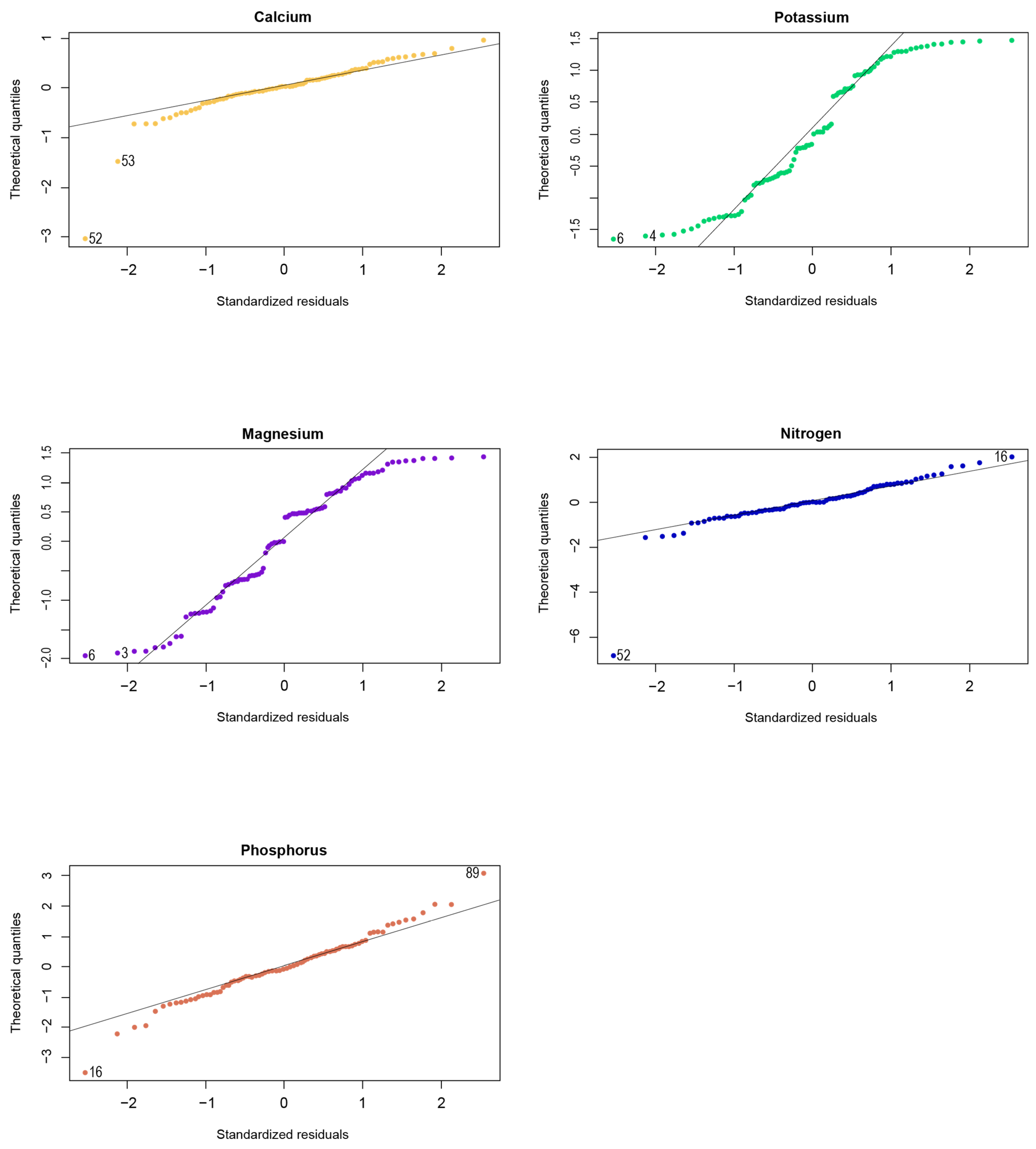
2.8. Statistical Analyses

The statistical analyses were performed with R version 4.1.0 [46]. The differences between the study areas were tested using the Welch two-sample t-test [47].

Whether greater soil acidity significantly affects the soil nutrient balance for all 10 sites, irrespective of the study area, was investigated for five nutrients (Ca, Mg, K, N, and P) using the F-test for nested linear models. Two linear models were fit to all five of the nutrient mass balances of all the sites: a full model with all relevant predictors, and a partial model with all relevant predictors except mean pH. More formally, the full model is as follows:

Y_{i k} = β_{1 k} + β_{2 k} x_{1 i} + \dots + β_{(p - 1) k} x_{(p - 2) i} + β_{p k} x_{(p - 1) i} + ϵ_{i k}

(3)

and the partial model is as follows:

Y_{i k} = β_{1 k} + β_{2 k} x_{1 i} + \dots + β_{(p - 1) k} x_{(p - 2) i} + ϵ_{i k}

(4)

where

x_{(p - 1)}

denotes mean pH,

x_{(1)}, \dots, x_{(p - 2)}

denotes the other predictors,

i = 1, \dots, n

indexes the observation,

k = 1, \dots, 5

indexes the nutrient, and

ϵ_{i k} \sim N (0, σ^{2})

is a random error term. The assumption that errors are normally distributed is necessary for the F-test. Hence, several transformations of the nutrient mass balances were compared, and the transformation that made the error Q-Q plot appear most reasonable was retained. Ca and N are transformed with

\log (Y + a)

, where

a = 1 - \min (Y)

makes the arguments to

l o g

positive. P is log-transformed without a corrective constant since all observations are non-negative, while K and Mg are left untransformed.

Y_{i k}

in the model thus represents the transformed mass balance for nutrient

k

. Q-Q plots are given in Appendix A (Figure A4).

The F-test pits

H_{0} : β_{p k}

= 0 (no effect) against

H_{A} : β_{p}

≠ 0 (effect). Under H₀,

F ≔ \frac{(S S E_{0} - S S E)}{S S E / (n - p)} \sim F_{1, n - p}

, where SSE is the sum of squared residuals under the full model and SSE₀ is the sum of squared residuals under the partial model. n is the number of observations and p is the number of coefficients in the full model. This test statistic was computed for every nutrient, then its p-value was obtained from the

F_{1, n - p}

distribution.

Finally, the Bonferroni–Holm correction was applied to account for multiple testing. This involves ordering the p-values of the individual tests in ascending order, then comparing them to an increasing sequence of p-value thresholds. Null hypotheses are sequentially rejected until the first failure to reject. Then, any remaining null hypotheses are also not rejected. The procedure controls the family-wise error rate (FWER), which we chose as

α = 0.05

. More details are available in [48].

3. Results

3.1. Site Conditions

No significant differences were found between the study areas for any of the parameters in Table 2. Although the tree roots in Bülach still reach the horizons with calcite, the pH values are only slightly higher than in Irchel. The average for the five sites in Bülach is 4.04 ± 0.24 and in Irchel, it is 3.90 ± 0.18 (Table 2). Irrespective of the study area, the pH values in the top 40 to 50 cm of the mineral soil fluctuate around 4 (Table A4). Accordingly, no significant differences were found for the site-specific mean base saturations between the two study areas. As both study areas contain sites with an occurrence of calcite relatively close to the soil surface, the mean base saturation in both areas varies between 30 and 96% (Table A4).

To obtain the value of the cation exchange capacity for the root zone, CEC was summed over all horizons of the depth of the root zone. As a result, it correlates closely with the depth of the root zone (r = 0.82) and, on the other hand, the organic carbon stock and the proportion of the clay fraction correlate closely with the CEC (r = 0.81 and 0.88 respectively, Table A5). The CEC shows no significant differences between the study areas and, combined with the base saturation, does not suggest any major differences in the stocks of basic cations. The stocks of Ca, Mg, and K vary over a similarly wide range when comparing the study areas (Table A4).

The stocks of extractable P and N show some of the highest variation within the study areas. Phosphorus varies between 98 and 3747 mmol·m⁻² in Bülach and between 43 and 290 mmol·m⁻² in Irchel (Table A4). Due to this large variation, the differences between the study areas are not significant. In the case of P, it is noticeable that the stocks at the Chengelboden, Lindi, and Marterloch sites in particular are larger than the largest stock in the Irchel study area (Table A4). Even if the difference between the study areas is not significant, the sites in Bülach tend to be richer in P than those in Irchel.

The main source of N is deposition from the atmosphere. As both study areas are geographically very close to each other (Table A1), the stocks of total N in both areas vary within a similar range and are independent of the underlying bedrock.

Contrary to the original assumptions, weathering is not lower in the older and more developed soils of the early Pleistocene than in the younger soils of the late Pleistocene (Table 3). The nutrient element loads in the leachate and the deposition of Ca, Mg, and K also do not differ significantly between the two study areas. On the other hand, N deposition is significantly higher in Bülach than in Irchel (24 vs. 20 kg·ha⁻¹·y⁻¹), but this does not lead to different stocks in the soil (see above).

There are also no significant differences in the leaching of basic cations between the study areas. Calcium is only leached at those sites where the root zone contains calcite and is therefore strongly correlated with the pH value in the root zone (Table A4 and Table A8). The leaching of Mg and K is 0–17.2 kg·ha⁻¹·y⁻¹ and 0–55.3 kg·ha⁻¹·y⁻¹, respectively. Both are relatively closely correlated with the CEC in the root zone (Table A4 and Table A8). P and N are hardly leached at all.

The similar weathering rate of both study areas is also related to the similar mineralogy in the soil. In general, the tills in this area originate from the erosion of a particular sequence of the alpine geology, geographically as well as stratigraphically. Since the erosion product is a mixture of lithologies, the bulk mineralogical composition of tills of different ages originally was comparable. The mineralogical composition of the C horizons on late Pleistocene till is characterized by higher carbonate, feldspar, and primary sheet silicate contents. As a result of the longer exposure to weathering of the substrate, C horizons on early Pleistocene till, on the other hand, are comparatively depleted in these minerals and exhibit higher clay and secondary mineral contents (Figure 1).

Regarding the export of nutrients due to harvesting, we tested the difference in element contents in tree components of beech between the two study areas (Figure 2). There is no significant difference in Ca in any tree compartment. The Ca contents are approximately the same in all tree components in both test areas. There is only one significant difference for Mg. The Mg contents in brushwood (<5 mm) are slightly higher in Bülach than in Irchel. The highest Mg contents in beech are found in the brushwood, while the bark is particularly rich in Ca. The greatest significant differences are found in the P contents. Corresponding to the generally higher P stocks in the soils in Bülach, the tree components have higher P contents in Bülach compared to Irchel. The differences are very significant in the bark and in fine (5–20 mm) and medium branches (20–70 mm), and even highly significant in brushwood (<5 mm). In contrast, the differences are only weakly to not significant in the coarse wood (Figure 2). The highest P contents are found in brushwood (<5 mm).

For the other elements (Figure A1), there are highly significant differences for K in the bark and further significant differences in the coarse branches (20–70 mm) and in the thin stem wood (70–120 mm). No significant differences were found for N. It is striking that the tree components in Irchel have higher contents of K than those in Bülach. Overall, however, the differences in the element contents of the tree components between the two study areas are small.

3.2. Biomass and Nutrient Export by Harvesting

Nevertheless, there are significant differences in the export of nutrients through timber harvesting for N and P. This is mainly due to the better growth of the trees on the early Pleistocene sites, which results in a higher exported biomass over the entire rotation period of 100 years (Figure 3). In the scenarios with low thinning intensity, significantly more biomass is harvested in the early Pleistocene sites than in the late Pleistocene sites for all three timber harvesting strategies. The same applies to stemwood harvesting with heavy thinning. As a result, more nutrients tend to be removed from stands in the early Pleistocene than from those in the late Pleistocene. These differences are significant for N and P for the timber harvesting strategies of whole trees and stems with branches with low thinning. For P, the differences between these two timber harvesting strategies are statistically confirmed even with heavy thinning. Mg and K show the same significant differences as P and additionally confirmed differences in stemwood harvesting with low thinning. There are no significant differences for Ca (Figure A2).

In all cases, whole-tree harvesting exports the most nutrients, followed by the harvesting strategies of stemwood with branches and stemwood only. In numbers, these are exported Ca quantities of between 14 and 22 kg·ha⁻¹·y⁻¹ for the whole-tree harvest, 13 to 21 kg·ha⁻¹·y⁻¹ for the harvest of stemwood with branches, and 11 to 18 kg·ha⁻¹·y⁻¹ for the harvest of stemwood only. The corresponding numbers for N are 10–15, 8–12, and 6–10 kg·ha⁻¹·y⁻¹. For Mg, the numbers are about 10 times lower than for Ca, and for K, they are about 3 times lower than for Ca. Phosphorus is exported the least in terms of quantity by timber harvesting, namely 0.7–1 kg·ha⁻¹·y⁻¹ for whole-tree harvesting, 0.5–0.7 kg·ha⁻¹·y⁻¹ for the harvesting of stemwood with thick branches, and 0.4–0.5 kg·ha⁻¹·y⁻¹ for stemwood harvesting.

Thus, all necessary element fluxes are available to calculate the nutrient balances from the sum of weathering and deposition reduced by the losses through leaching and nutrient exports by timber harvesting. The mass balances tend to be larger in Bülach (late Pleistocene) than in Irchel (early Pleistocene). However, the differences are only significant for N (for all nine management strategies; Figure 4). For all thinning and timber harvesting scenarios, there are significantly greater positive N balances in the late Pleistocene than in the early Pleistocene. There are no significant differences for any other nutrients (Figure 4 for Ca, Figure A3 for Mg, K, and P). Because the largest quantities of elements are exported during whole-tree harvesting, the overall mass balances are smaller for whole-tree harvesting than for stemwood with thick branches and stem-only harvesting. The mass balances differ only marginally between the various thinning intensities and primarily reflect the differences in the harvested biomass. It is therefore noticeable that for the weakest thinning in Irchel with the largest harvested biomass, the mass balances tend to be lower than for the stronger thinning intensities.

All Ca balances are negative, even if only stemwood is harvested (Figure 4). In the Ca data in Figure 4, the values for the site “Brengspel” in Bülach (late Pleistocene) are not included, because they are considered as outliers. At this site, calcite is already present at a depth of 0.4 m, which leads to extremely high Ca weathering in the root zone. If the site “Brengspel” were to be included in the balancing, the average Ca balances would be positive, but with a very large standard error. On the sites of the early Pleistocene, the mass balances of P are negative for all three thinning intensities with whole-tree harvesting (Figure A3). The mass balances without timber harvesting, on the other hand, are positive for all elements and management strategies without exception.

3.3. Dependence of Nutrient Balance on Acidification

So far, the differences in the mean values between the two study areas have been tested for significance. As the variability within the study areas is as large as across both study areas combined, only very few properties were significantly different. We therefore tested the statistical relationship between acidification, expressed by pH in the root zone, and the nutrient balances of five nutrients for all 10 sites, irrespective of the study area.

The statistical procedure in Section 2.8 produced ten linear model fits, whose coefficients are reported in Table A10 with associated significance levels in Table A11. Subsequently, five F-tests were conducted, and their p-values were compared with the Bonferroni–Holm-adjusted significance level. Table A11 reports the p-values from the test. This led to the rejection of

H_{0}

(no effect) for Ca and Mg but failure to reject

H_{0}

for K, P, or N. Coupled with the pH coefficient estimates in the linear models, we conclude that higher soil pH is associated with a higher Ca mass balance and a lower Mg mass balance, and we cannot reject the possibility of no association for the other three nutrients. Figure 5 illustrates that despite the failure to reject

H_{0}

, an association between soil pH and K, P, or N remains plausible, with the association appearing positive for N and negative for K and P.

4. Discussion

Balancing the nutrient fluxes of weathering, deposition, leachate loss, and nutrient removal through timber harvesting provides information regarding the influence of timber harvesting on the nutrient sustainability of the sites. The sites in our two study areas are very heterogeneous (in terms of acidification), although the geological conditions within the study area were mapped as homogeneous. Neither in most of the individual nutrient fluxes nor in most of the nutrient balances were significant differences between the study areas of the early versus late Pleistocene identified. This has mainly two reasons: (1) Despite differences in annual precipitation of 500 mm and tills from different geological periods forming the bedrock, similar soils with similar properties have been formed in both study areas. (2) The spatial variability of soil properties within the study areas is as large as the total variability across both study areas. On the other hand, soil acidification at all sites, regardless of the study area, expressed by the pH value of the soil, has a significant influence on the nutrient balances.

Contrary to our assumptions, the soils of the early Pleistocene are not more weathered and not very different in nutrients due to the longer time of soil development than the soils of the late Pleistocene. In principle, stronger weathering leads to the stronger depletion of easily weatherable mineral components, while more weather-resistant (i.e., more siliceous) components persist. This evidently does not affect the overall weathering rate or the nutrient content of the soils. Neither is the case in our study. However, both the weathering rate and the nutrient stocks in the root zone vary substantially in the two study areas. This is partly due to the great variability in soil properties within the two study areas, especially on the Irchel Plateau. The Irchel Plateau consists of flat-lying gravels of the early Pleistocene, which break off at the edge of the plateau. Carbonate-bearing molasse sediments are exposed on the steep slopes below the plateau [14]. At the edges of the plateau, the carbonate-containing sediments are closer to the soil surface than in the center of the plateau due to erosion of the gravels of the early Pleistocene. This applies to two sites (Schartenflue and Schaffhuser), where the occurrence of calcite is at depths of 1 and 0.8 m, respectively, in contrast to the three profiles in the center of the plateau, where the depth of the occurrence of calcite could not be reached with the soil profiles and had to be determined by drilling.

This leads to great variability in the chemical properties of the soil and, in particular, the nutrient stocks in the root zone. The element stocks are positively correlated with the depth of calcite but even more strongly positively correlated with the thickness of the root zone. This is a critical point in the calculation of nutrient balances. The root zone was assumed to be thick, as tree roots could be observed in the open soil profile. This leads to a certain degree of randomness, as a soil profile is not necessarily representative of the entire root zone of a tree. However, it was the method of choice, as the nutrient uptake by the trees, estimated by the uptake rate and the observed rooting density, significantly influences the result of the modeling of weathering and leachate losses in feed-back loops [29]. If we had assumed a standard depth of the root zone, we would have had to assume rooting intensities for the deeper horizons that may have nothing to do with reality.

Although the average depth of the root zone in both study areas is 1.2 m (Table 1), the sites at Irchel seem to tend to have slightly larger stocks of basic cations (Ca, Mg, and K) than those in Bülach. Pedological explanations can be found for these tendencies. With comparable pH values around 4 and thus comparable acidification in the root zone, the average CEC and the clay fraction in Irchel is about twice as high as in Bülach. This can be attributed to the longer period of soil formation in Irchel with a more pronounced formation of secondary clay minerals. This also means that there are more negatively charged sites to bind basic cations in an exchangeable form, which are located on the surfaces of the clay minerals. In particular, Mg and K correlate very closely with the size of the clay fraction (r = 0.97 and 0.95, respectively), whereas Ca correlates less (r = 0.17; Table A3). At the same time, acidification is not yet so advanced that clay minerals would be destroyed to any significant extent.

In Bülach, the soils are clearly, although not significantly, richer in Lakanen-extractable P. Numerous studies have investigated the relationship between the age of soil development and the P content of soils [12,49,50,51]. Turner and Laliberté [12] investigated a chrono-sequence in southwestern Australia (6500 to 2 million years) and demonstrated that total P (TP) in the soil decreased continuously with increasing soil age. In addition, they found that the ratios of soil organic carbon (SOC)–TP and TN:TP increased steadily as soil development progressed. They concluded that N is limiting during the early stages of soil development and that this gradually shifts to P limitation as soil development progresses. This corresponds well to the conditions in our test areas. The younger soils of the late Pleistocene have larger P stocks than those of the early Pleistocene in the Irchel, which have been able to develop for several hundreds of thousands of years.

The relations of nutrient stocks in the soil are very well reflected in the nutrient contents of the tree components. While the marginal differences in the soil stocks of Ca, Mg, K, and N also result in marginal, non-significant differences in the corresponding element contents in the tree components, the P contents in the tree components of the two study areas differ significantly, although the soil stocks of P only tend to be greater in the late Pleistocene sites. This is difficult to interpret, as the influence of the site on the element contents in the trees is often overlaid by other effects such as stand age or climate [52].

The distribution of nutrient elements within the beech trees is largely consistent with values from the literature. The physiologically most active components have the highest nutrient element contents. The Ca contents in the bark are significantly higher than those in the brushwood, branches and merchantable wood. This is consistent with the results of other authors [6,53,54]. However, while these authors also found the highest contents of K, Mg, and N in the bark, the contents in the brushwood (<5 mm) are the highest in our investigations. This can be explained by the sampling of the tree components. While in the aforementioned studies the contents in the branches < 7 cm were investigated, we divided this compartment into three parts and thus no dilution in the finest branches was achieved due to a large proportion of wood. Ulbricht et al. [55] also sampled the branches < 7 cm in three diameter categories and found a ranking of the contents in the components in P identical to our results. Furthermore, the time of sampling could also be a possible reason for the ranking to change. However, according to the study by Ulbricht et al. [55], the ranking of the nutrient contents in the tree components does not change between summer and winter sampling.

To determine the nutrient exports through wood harvesting, the nutrient contents of the tree components are multiplied by the modeled biomass. There may be several reasons for the higher biomass accumulation in Irchel compared to Bülach. Although the soils on the Irchel Plateau are more acidified and at least partially poorer in nutrients than in Bülach, the growth of the tree species occurring in the stands may be greater than on the less acidified sites in Bülach. The site class as an expression of the combined effect of all site factors (not just soil chemistry) is obviously greater in Irchel than in Bülach. It is possible that in favorable climate conditions (slightly cooler but significantly more humid), some biological adaptation processes, such as an efficient root colonization as well as an efficient nutrient cycling, may allow for the maintenance of stand growth and nutrition of soils with low nutrient reserves [56]. In addition, the stands in Bülach and Irchel differ in terms of tree species composition and stem number. The number of stems per hectare in Irchel is slightly lower than in Bülach. This could be a result of interspecific competition, which is higher in Irchel compared to Bülach. A third reason could be a different upscaling effect in Irchel and Bülach from the plot to the stand level.

This management effect is even more pronounced with the “LOW” thinning intensity. In the Irchel test area, tree growth is larger over the entire rotation period of 100 years with the “LOW” scenario than with more intensive thinning. This can be explained by (1) different reactions of the stands to the thinning intensity, (2) the tree species composition of the stands, and (3) possible uncertainties of the SwissStandSim model predictions. (1): A low thinning intensity is not necessarily associated with a lower timber harvest volume over the whole rotation cycle. It is possible that with more intensive thinning, a later possible increment is already skimmed off prematurely due to increased removal of the “means of production” of individual stems. Mey et al. [45] have also shown a similar correlation. (2): This first point can be illustrated very well with the admixture of Douglas-fir in the stands in Irchel. Douglas-fir is a tree species that can still achieve superior growth compared to beech even at an older age [57,58]. On the one hand, if it is heavily intervened with at an early stage, later growth is limited. On the other hand, under low thinning intensity, more Douglas-firs remain in the stand, which can lead to increased biomass after the end of the rotation period. (3): The accuracy of model predictions may be limited by the amount of data used for model parametrization, especially for Douglas-fir which is not very common in the Swiss forest and not much empirical data is available.

As the nutrient fluxes relevant for balancing do not differ significantly in most cases, not many significant differences in the overall balances can be expected. The exception is a significant difference for N that can be explained by the fact that N is mainly introduced into the forest ecosystem by deposition. Nitrogen deposition is significantly greater in Bülach (late Pleistocene) than in Irchel (early Pleistocene). Depending on the specific site, the N deposited is biologically fixed to a large extent [59], so that losses through leaching are low. The mean estimated value for N leaching via percolating water from forest areas in a study of 2005 for north-eastern Switzerland in the vicinity of our study area is 0 to 1 kg N·ha⁻¹·yr⁻¹ [60]. In addition to the lower N deposition in Irchel, more biomass is exported at the early Pleistocene sites, which leads to significantly more positive N balances in the late Pleistocene sites.

Whole-tree harvesting leads to significantly greater nutrient removal than the other two harvesting strategies. With the whole-tree harvest, an average of 3 to 4 kg·ha⁻¹·yr⁻¹ more Ca is exported in both study areas compared to the pure stemwood harvest, which reduces the balances accordingly. For N, these values are even 4 to 5 kg·ha⁻¹·yr⁻¹; for K, 1 to 5 kg·ha⁻¹·yr⁻¹; and for Mg and P, still 0.3 to 0.5 kg·ha⁻¹·yr⁻¹. This has an impact on biodiversity and on the resistance and resilience of forest ecosystems. The most obvious effect on biodiversity is the reduction in wood-inhabiting species [3]. A balanced nutrient mass balance is important for the resistance and resilience of the forest to external factors such as drought stress, wind, or insect calamities [11]. For the resilience of forest ecosystems, nutrient sustainability, or the maintenance of soil fertility after wood use, is an important aspect. In the case of alkaline cations, the resilience of forest ecosystems to wood utilization is ensured by weathering, which is the most important source of alkaline cations [61]. The mass balances for Ca are negative in both test areas for all nine wood harvesting strategies and for P in the Irchel test area for the whole-tree harvesting. This means that neither resistance nor resilience are still conferred.

The lack of influence of the geological substrate on the nutrient sustainability of timber harvesting is mainly due to the variability within the geological units. The variability within the study areas is about the same as the variability of all sites in both study areas. In order to determine the site parameters that influence the mass balances and that can help to find the right management measures, this variability must be taken into account. This means that in addition to the yield parameters and external large-scale nutrient fluxes, soil properties that are directly related to the nutrient supply of the trees must also be taken into account. We showed that a higher soil pH is associated with a higher Ca mass balance and a lower Mg mass balance.

Figure 5 illustrates a caveat to the statistical analysis. There is a high variance in the nutrient mass balance within sites. If any of the variation can be attributed to measurement error, then this would obscure the underlying relationship between nutrient mass balance and soil pH. A further caveat to the statistical analysis is visible in Figure A4. Despite the normalizing transformations, none of the models have a “textbook” straight-line QQ plot, indicating that the assumption of normal errors may not be upheld.

5. Conclusions

Our results show that detailed soil data and data on the entire nutrient cycle are essential for assessing nutrient sustainability, an important basis for close-to-nature forestry. Information from relatively large-scale maps is not sufficient, as the variability within the mapping units is too big. Site-specific data are therefore needed. If, in addition to the mapping unit, just the pH value of the soil as an important parameter of soil acidification is known, the nutrient sustainability and mass balances for different forest management scenarios can be predicted much better.

The assumed depth of the root zone has proven to be a critical factor in estimating nutrient balances. With increasing thickness of the assumed root zone, the mean pH value of the soil is increasing and the influence of the depth of the presence of calcite becomes greater, which significantly improves the Ca balance in particular.

At the investigated sites of the early and late Pleistocene, full-tree harvesting in particular has negative consequences for nutrient sustainability. With this harvesting method, the balances for Ca and P are negative at all thinning intensities. In all other forest management scenarios, only Ca appears to be problematic.

Author Contributions

Conceptualization, S.Z., D.K., and J.S.; methodology, S.Z., D.K., T.T., R.M., N.T.P., and J.S.; software, D.K., T.T., R.M., and M.P.; validation, S.Z. and J.S.; formal analysis, S.Z. and N.T.P.; investigation, S.Z.; resources, S.Z.; data curation, S.Z., D.K., and J.S.; writing—original draft preparation, S.Z., J.S., and D.K.; writing—review and editing, D.K., T.T., R.M., N.T.P., and M.P.; visualization, S.Z.; supervision, J.S. and D.K.; project administration, S.Z.; funding acquisition, S.Z. All authors have read and agreed to the published version of the manuscript.

Funding

This research was funded by Swiss Forest and Wood Research Promotion Agency (WHFF-CH), grant number 01.0101.PZ/0005/2020.2, and by the Conference for Forest, Wildlife and Landscape (KWL), grant number KWL-2020.02, which are both gratefully acknowledged.

Data Availability Statement

The original data presented in the study are openly available in EnviDat (https://www.envidat.ch/#/; accessed on 10 June 2024) at https://doi.org/10.16904/envidat.505 (accessed on 10 June 2024).

Acknowledgments

The authors would like to thank the two foresters of Bülach (Thomas Kuhn) and Irchel (Hans Beereuter) for their help with the field work and the felling of the trees. Nathalie Barengo from the Forest Department of the Zurich Cantonal Administration provided the stand inventory data for Bülach and Irchel. Golo Stadelmann helped with the selection of the models used in this study and Ubald Gasser from Bodenschutz Zürich assisted with the selection of the study sites. The great support of Marco Walser, Roger Köchli, Behzad Rahimi, Daniel Christen, and Alois Zürcher in the field and laboratory work is also gratefully acknowledged. The suggestions by two anonymous reviewers are also gratefully acknowledged.

Conflicts of Interest

The authors declare no conflicts of interest.

Appendix A

Table A1. Site characteristics, tree species, soil type, and geological unit of the two study areas Bülach and Irchel. Tree species: Acer pseudoplatanus L. (BAh), Tilia cordata Mill. (Li), Quercus robur L. (Ei), Fagus sylvatica L. (Bu), Abies alba Mill. (Ta), Picea abies (L.) H. Karst. (Fi), Pinus sylvestris L. (Fö), Larix decidua Mill. (Lä), Fraxinus excelsior L. (Es), and Pseudotsuga menziesii (Mirb.) Franco (Dougl).

Study Area	Site Name	Longitude	Lattitude	Altitude [m]	Exposure	Slope [%]	Tree Species	Soil Type	Geological Unit
Bülach	Lärchenischlag	8.52747	47.52564	428	NW	7	Bu, BAh, Li	Calcic Luvisol	Late Pleistocene
	Chengelboden	8.52879	47.53423	435	SE	3	Bu, Ta, Fi, BAh	Dystric Cambisol
	Lindi	8.53340	47.54641	423	-	0	Bu, Fö, Fi, BAh	Calcic Luvisol
	Marterloch	8.53648	47.53980	432	-	0	Bu, Fi, Fö	Calcic Luvisol
	Brengspel	8.53650	47.53054	451	-	1	Bu, BAh, Fö, Lä, Ei	Calcaric Cambisol
Irchel	Hörnli	8.58262	47.55627	676	-	0	Bu, Ei, Fi	Haplic Luvisol	Early Pleistocene
	Schartenflue	8.59637	47.54898	668	-	2	Bu, Ei	Calcic Luvisol
	Schaffhuser	8.60396	47.54749	669	NE	50	Bu, Fi, Es	Eutric Cambisol
	Obermeser	8.61025	47.53738	692	NW	2	Bu, Fi, Dougl	Haplic Luvisol
	Steig	8.61735	47.53603	680	W	3	Bu, Fi, Dougl	Haplic Luvisol

Table A2. Morphological soil properties of the 5 sites in the study area Bülach. Texture classes: Ss = pure sand, Slu = silty-loamy sand, Sl = loamy sand, St = clayey sand, Ls = sandy loam, Lts = sandy clayey loam, Lu = silty loam.

Site	Pedogenetic Horizon and Its Depth [cm]	Stone Content [%]	Texture	Density of the Fine Earth [Mg·m⁻³]	Hydromorphic Features	Soil Color
Lärchenischlag	L (1.5–0)	-	-	0.10	no	-
	Ah (0–10)	11–25	Sl	0.67	no	10YR 3/3
	(E)AB (10–30)	26–50	Sl	0.72	no	10YR 4/4
	B(t) (30–50)	51–75	Lts	0.74	no	10YR 4/6
	CBv (50–80)	51–75	Sl	0.78	no	10YR 5/6
	Cca1 (80–110)	>75	Ss	0.78	no	10YR 5/2
	Cca2 (110–135)	>75	Ss	0.81	no	10YR 5/2
Chengelboden	L (3–0.5)	-	-	0.10	no	-
	[F] (0.5–0)	-	-	0.15	no	-
	Ah (0–6)	<2	Slu	0.91	no	10YR 2/3
	(A)B (6–20)	<2	Lu	0.91	no	10YR 4/4
	Bv (20–40)	11–25	Lu	1.19	no	10YR 5/4
	BSw (40–60)	<2	Lu	1.28	Mn concretions	10YR 6/3
	Sw (60–100)	<2	Lu	1.49	Mn concretions	2.5Y 6/4
	IISw (100–140)	<2	Ls	1.55	pale-red colors	2.5Y 5/4
	IISd (140–195)	<2	Ls	1.59	pale-red colors	2.5Y 5/3
	IICca (195–220)	>75	Sl	1.46	no	10YR 5/2
Lindi	L (3–1)	-	-	0.10	no	-
	F (1–0)	-	-	0.15	no	-
	Ah (0–4)	<2	Sl	0.88	no	10YR 3/3
	(EA)B (4–20)	<2	Ls	0.88	no	10YR 4/4
	(E)B (20–40)	2–10	Ls	1.17	no	10YR 5/6
	B(t) (40–55)	2–10	Ls	0.87	no	10YR 5/6
	CB(t) (55–80)	26–50	Lts	0.87	no	10YR 4/6
	B(t) (80–100)	<2	Sl	1.33	no	10YR 5/6
	Cca (100–155)	>75	Sl	1.20	no	10YR 6/3
Marterloch	L (1–0)	-	-	0.10	no	-
	Ah (0–5)	2–10	Sl	0.91	no	10YR 2/3
	(EA)B (5–25)	11–25	Ls	0.91	no	10YR 4/3
	(E)B(cn) (25–60)	11–25	Lu	1.09	Mn concretions	10YR 5/6
	B(t,cn) (60–80)	26–50	Lts	1.10	Mn concretions	10YR 4/4
	CB(t) (80–105)	51–75	Lts	0.95	no	10YR 4/4
	Cca (105–140)	>75	St	0.95	no	10YR 6/1
Brengspel	L (1–0)	-	-	0.10	no	-
	Ah (0–15)	11–25	Sl	0.67	no	10YR 3/2
	(A)B (15–30)	26–50	Sl	0.72	no	10YR 4/4
	AB (30–40)	>75	Ls	0.79	no	10YR 4/6
	Cca1 (40–70)	>75	Sl	0.71	no	10YR 5/4
	Cb,ca (70–90)	<2	Sl	1.15	no	10YR 6/2

Table A3. Morphological soil properties of the 5 sites in the study area Irchel. Texture classes: Sl = loamy sand, St = clayey sand, Ls = sandy loam, Lts = sandy clayey loam, Lt = clayey loam.

Site	Pedogenetic Horizon and Its Depth [cm]	Stone Content [%]	Texture	Density of the Fine Earth [Mg·m⁻³]	Hydromorphic Features	Soil Color
Hörnli	L (1–0)	-	-	0.10	no	-
	Ah (0–6)	<2	Sl	0.99	no	10YR 3/2
	(A)B (6–25)	<2	Ls	0.99	no	10YR 4/4
	(Sw)B (25–65)	2–10	Ls	1.41	Mn concretions	10YR 4/6
	Sd1 (65–90)	11–25	Lt	1.41	Mn concretions	10YR 6/8
	Sd2 (90–160)	26–50	Lt	1.44	Mn concretions	10YR 5/6
	Sd3 (160–225)	26–50	Lt	1.51	Mn concretions	10YR 5/6
Schartenflue	L (2–0)	-	-	0.10	no	-
	Ah (0–6)	26–50	Sl	0.59	no	10YR 3/2
	(E)AB (6–15)	26–50	Sl	0.59	no	10YR 4/3
	(E)Bv (15–40)	26–50	Sl	0.85	no	10YR 5/6
	(E)CBv (40–60)	51–75	Sl	1.08	no	10YR 4/6
	(Bt)C (60–100)	>75	Lts	1.08	no	10YR 4/6
	Cca (100–140)	>75	St	1.13	no	10YR 5/2
Schaffhuser	L (2–0)	-	-	0.10	no	-
	Ah (0–10)	11–25	Lts	0.67	no	10YR 3/2
	(E)AB (10–20)	11–25	Ls	0.72	no	10YR 4/2
	B(t) (20–40)	11–25	Lts	0.89	no	10YR 5/4
	Bcn (40–55)	11–25	Lt	1.06	Mn concretions	10YR 6/6
	CB (55–80)	51–75	Lts	0.91	no	10YR 5/6
	(Bcn)Cca (80–120)	<2	Lts	1.36	Mn concretions	10YR 6/4
	Rca (120–130)	>75	-	1.47	no	-
Obermeser	L (1.5–0)	-	-	0.10	no	-
	Ah (0–6)	11–25	Sl	0.72	no	10YR 4/2
	(EA)B (6–16)	11–25	Ls	0.72	no	10YR 4/4
	(E)Bcn1 (16–35)	11–25	Ls	1.04	Mn concretions	10YR 6/6
	(E)Bcn2 (35–50)	11–25	Ls	1.04	Mn concretions	10YR 5/4
	B(t),cn (50–65)	11–25	Ls	1.24	Mn concretions	10YR 5/6
	Sw (65–95)	11–25	Lt	1.21	Mn concretions	10YR 6/6
	Sd (95–130)	11–25	Lt	1.34	Mn concretions	10YR 5/6
	SdC (130–220)	51–75	Ls	1.30	Mn concretions	10YR 5/8
Steig	L (2–0.5)	-	-	0.10	no	-
	F (0.5–0)	-	-	0.15	no	-
	A (0–15)	11–25	Ls	0.98	no	10YR 3/2
	ElB (15–40)	11–25	Lt	1.15	no	10YR 6/6
	Bt (40–140)	11–25	Lts	1.35	Mn concretions	7.5YR 5/6
	BC (140–200)	11–25	Lts	1.43	Mn concretions	10YR 4/6

Table A4. Mean values in the considered rooting zone of the sites on early Pleistocene of pH; base saturation (BS); cation exchange capacity (CEC); clay fraction; organic carbon stock; stock of exchangeable calcium (Ca_exc), magnesium (Mg_exc), and potassium (K_exc); extractable phosphorus (P_lak [19]); as well as the stock of total nitrogen (N_tot). An extended version of this table is available under https://doi.org/10.16904/envidat.505 (accessed on 10 June 2024).

Soil Property	Lärchenischlag	Chengelboden	Lindi	Marterloch	Brengspel	Hörnli	Schartenflue	Schaffhuser	Obermeser	Steig
Mean pH-value	4.05	3.76	3.72	3.70	4.96	3.72	3.83	4.59	3.61	3.77
Mean BS [%]	62.6	53.3	29.9	29.8	96.3	34.5	38.0	96.2	31.6	33.0
CEC [mol_c·m⁻²]	23.2	143.7	53.2	52.9	69.6	74.0	15.5	242.1	162.4	305.0
Amount of clay [kg·m⁻²]	47.1	430.2	165.2	175.3	61.4	222.8	39.2	278.0	380.6	796.8
Stock of C_org [kg·m⁻²]	4.7	7.4	7.2	5.5	7.1	5.7	4.1	7.7	7.6	8.3
Ca_exc [mol·m⁻²]	6.8	23.2	4.7	5.4	32.9	6.3	2.4	111.9	15.5	24.9
Mg_exc [mol·m⁻²]	0.30	12.92	2.60	1.89	0.42	5.67	0.47	2.67	8.62	22.89
K_exc [mol·m⁻²]	0.26	3.74	0.99	1.01	0.42	1.52	0.16	3.16	3.11	4.96
P_lak [mmol·m⁻²]	98.3	3746.7	960.4	582.6	279.7	49.3	43.4	152.0	441.7	290.2
N_tot [mol·m⁻²]	22.1	73.4	39.9	33.5	33.4	29.9	16.7	44.4	47.2	76.8

Table A5. Correlation matrix (Pearson correlation coefficient) of CEC, depth of the root zone, amount of clay, stock of C_org, Ca_exc, Mg_exc, and K_exc.

Correlation Matrix	CEC [mol_c·m⁻²]	Depth of Root Zone [m]	Amount of Clay [kg·m⁻²]	Stock of C_org [kg·m⁻²]	Ca_exc [mol·m⁻²]	Mg_exc [mol·m⁻²]	K_exc [mol·m⁻²]
CEC [mol_c·m⁻²]	1
Depth of root zone [m]	0.82	1
Amount of clay [kg·m⁻²]	0.88	0.87	1
Stock of C_org [kg·m⁻²]	0.81	0.77	0.71	1
Ca_exc [mol·m⁻²]	0.60	0.25	0.17	0.49	1
Mg_exc [mol·m⁻²]	0.77	0.84	0.97	0.62	4.2 × 10⁻³	1
K_exc [mol·m⁻²]	0.93	0.81	0.95	0.78	0.39	0.89	1

Table A6. Weathering rate of Ca, Mg, K, and P at all sites of the two study areas for all three different thinning intensities.

Site	Study Area	Thinning Intensity	Ca [kg·ha⁻¹·y⁻¹]	Mg [kg·ha⁻¹·y⁻¹]	K [kg·ha⁻¹·y⁻¹]	P [kg·ha⁻¹·y⁻¹]
Lärchenischlag	Bülach	HIGH	12.26	1.09	3.61	0.39
Chengelboden			13.56	19.44	69.99	4.07
Lindi			2.96	4.46	13.39	0.86
Marterloch			3.17	5.89	14.71	1.00
Brengspel			549.49	2.34	3.72	0.61
Hörnli	Irchel		1.68	5.25	14.75	0.00
Schartenflue			0.54	0.48	1.40	0.14
Schaffhuser			624.39	8.59	10.03	0.36
Obermeser			1.90	11.14	39.81	0.00
Steig			3.09	19.58	64.28	0.00
Lärchenischlag	Bülach	LOW	12.25	1.08	3.56	0.39
Chengelboden			13.54	19.42	69.88	4.07
Lindi			2.96	4.46	13.42	0.86
Marterloch			3.17	5.88	14.65	1.00
Brengspel			549.88	2.35	3.74	0.61
Hörnli	Irchel		1.69	5.27	14.86	0.00
Schartenflue			0.54	0.48	1.40	0.14
Schaffhuser			624.09	8.59	10.01	0.36
Obermeser			1.90	11.14	39.80	0.00
Steig			3.09	19.60	64.38	0.00
Lärchenischlag	Bülach	BAU	12.26	1.09	3.61	0.39
Chengelboden			13.55	19.44	69.97	4.07
Lindi			2.96	4.46	13.42	0.86
Marterloch			3.17	5.89	14.71	1.00
Brengspel			549.57	2.35	3.73	0.61
Hörnli	Irchel		1.68	5.26	14.80	0.00
Schartenflue			0.54	0.48	1.40	0.14
Schaffhuser			624.29	8.59	10.02	0.36
Obermeser			1.90	11.13	39.79	0.00
Steig			3.09	19.58	64.29	0.00

Table A7. Deposition of Ca, Mg, K, P, and N at all sites of the two study areas. The deposition is the same for all three different thinning intensities.

Site	Study Area	Ca [kg·ha⁻¹·y⁻¹]	Mg [kg·ha⁻¹·y⁻¹]	K [kg·ha⁻¹·y⁻¹]	P [kg·ha⁻¹·y⁻¹]	N [kg·ha⁻¹·y⁻¹]
Lärchenischlag	Bülach	6.37	0.67	2.82	0.74	25.35
Chengelboden		6.31	0.67	2.78	0.74	22.41
Lindi		6.14	0.65	2.65	0.74	24.51
Marterloch		6.20	0.65	2.70	0.74	22.44
Brengspel		6.30	0.67	2.77	0.74	24.73
Hörnli	Irchel	6.18	0.65	2.64	0.73	18.61
Schartenflue		6.18	0.65	2.64	0.73	18.85
Schaffhuser		6.30	0.67	2.73	0.73	20.67
Obermeser		6.15	0.65	2.62	0.73	21.04
Steig		6.21	0.66	2.67	0.73	20.88
Lärchenischlag	Bülach	6.37	0.67	2.82	0.74	25.35
Chengelboden		6.31	0.67	2.78	0.74	22.41
Lindi		6.14	0.65	2.65	0.74	24.51
Marterloch		6.20	0.65	2.70	0.74	22.44
Brengspel		6.30	0.67	2.77	0.74	24.73
Hörnli	Irchel	6.18	0.65	2.64	0.73	18.61
Schartenflue		6.18	0.65	2.64	0.73	18.85
Schaffhuser		6.30	0.67	2.73	0.73	20.67
Obermeser		6.15	0.65	2.62	0.73	21.04
Steig		6.21	0.66	2.67	0.73	20.88
Lärchenischlag	Bülach	6.37	0.67	2.82	0.74	25.35
Chengelboden		6.31	0.67	2.78	0.74	22.41
Lindi		6.14	0.65	2.65	0.74	24.51
Marterloch		6.20	0.65	2.70	0.74	22.44
Brengspel		6.30	0.67	2.77	0.74	24.73
Hörnli	Irchel	6.18	0.65	2.64	0.73	18.61
Schartenflue		6.18	0.65	2.64	0.73	18.85
Schaffhuser		6.30	0.67	2.73	0.73	20.67
Obermeser		6.15	0.65	2.62	0.73	21.04
Steig		6.21	0.66	2.67	0.73	20.88

Table A8. Leaching of Ca, Mg, K, P, and N at all sites of the two study areas for all three different thinning intensities.

Site	Study Area	Thinning Intensity	Ca [kg·ha⁻¹·y⁻¹]	Mg [kg·ha⁻¹·y⁻¹]	K [kg·ha⁻¹·y⁻¹]	P [kg·ha⁻¹·y⁻¹]	N [kg·ha⁻¹·y⁻¹]
Lärchenischlag	Bülach	HIGH	1.50	0.00	0.00	0.08	0.00
Chengelboden			0.00	15.20	55.28	0.08	0.00
Lindi			0.00	1.87	4.33	0.08	0.00
Marterloch			0.00	3.01	5.90	0.08	0.00
Brengspel			446.02	0.07	0.00	0.08	0.00
Hörnli	Irchel		0.00	3.11	7.25	0.08	0.00
Schartenflue			0.00	0.00	0.00	0.08	0.00
Schaffhuser			606.01	5.78	2.49	0.08	0.00
Obermeser			0.00	8.57	29.57	0.08	0.00
Steig			0.00	17.17	55.02	0.08	0.00
Lärchenischlag	Bülach	LOW	2.39	0.00	0.00	0.08	0.04
Chengelboden			0.00	15.63	56.69	0.08	0.00
Lindi			0.00	1.66	3.50	0.08	0.00
Marterloch			0.00	3.18	6.42	0.08	0.00
Brengspel			443.87	0.06	0.00	0.08	0.00
Hörnli	Irchel		0.00	2.57	5.33	0.08	0.00
Schartenflue			0.00	0.00	0.00	0.08	0.00
Schaffhuser			607.29	6.00	3.22	0.08	0.00
Obermeser			0.00	8.63	29.70	0.08	0.00
Steig			0.00	16.78	53.69	0.08	0.00
Lärchenischlag	Bülach	BAU	1.38	0.00	0.00	0.08	0.00
Chengelboden			0.00	15.30	55.65	0.08	0.00
Lindi			0.00	1.69	3.67	0.08	0.00
Marterloch			0.00	3.01	5.84	0.08	0.00
Brengspel			445.62	0.07	0.00	0.08	0.00
Hörnli	Irchel		0.00	2.90	6.52	0.08	0.00
Schartenflue			0.00	0.00	0.00	0.08	0.00
Schaffhuser			606.36	5.87	2.75	0.08	0.00
Obermeser			0.00	8.68	29.91	0.08	0.00
Steig			0.00	17.12	54.84	0.08	0.00

Table A9. Summary of the modeled mineralogical composition of the C horizons of all soil profiles in the two study areas (unit: wt. %). Abbreviations: qz: quartz, fsp: feldspars, crb: carbonates, feo: Fe-oxides and -hydroxides, shs: sheet silicates (including biotite, muscovite, and chlorite), cm: clay minerals (including illite, smectite, vermiculite, and kaolinite), om: organic matter. Irchel: bedrock early Pleistocene till, Bülach: bedrock late Pleistocene till.

Site	Horizon	Depth [m]	qz	fsp	crb	feo	shs	cm	om
Irchel
Steig	BcnC	1.6–1.8	55.75	0.54	0	5.17	4.14	34.56	0.09
Hörnli	Sd	1.8–2.25	56.65	4.5	0	5.01	2.45	32.12	0.01
Schartenflue	Rcca	1.1–1.4	58.82	5.07	18.35	1.9	5.6	10.53	0.15
Obermeser	SdC	1.3–1.6	66.44	1.24	0	3.28	2.98	25.57	0.29
Schaffhuser	Cca	0.9–1.1	34.49	5.92	30.22	3.6	0	26.05	0.05
Bülach
Lärchenischlag	Cca2	1.2–1.35	48.48	14.39	26.65	0.94	5.6	3.52	0.81
Chengelboden	IICca	1.95–2.2	33.05	14.06	29.6	2.62	8.01	12.5	0.2
Brengspel	Cca2	1.0–1.2	30.76	7.15	42.4	0.67	6.21	13.21	0.09
Marterloch	Cca	1.2–1.4	50.6	6.33	23.77	1.77	9.83	8.02	0.14
Lindi	B	0.85–0.95	57.46	17.44	0.2	2.09	10.54	13.06	0.16

Table A10. Coefficients of nutrient mass balance models.

Full vs. Partial Model	Response Mass Balance	Thinning HIGH	Thinning LOW	Timber Harvesting (Stem Only)	Timber Harvesting (Whole Tree)	Depth of Occurrence of Calcite	Depth of the Rooting Zone	Late Pleistocene	Mean CEC	Mean pH
Full	Ca	0.07	−0.20	0.12	−0.12	−0.27	1.72	0.07	−0.01	1.14
Partial	Ca	0.07	−0.20	0.12	−0.12	−0.94	2.33	−0.21	−0.01	−
Full	N	0.03	−0.10	0.13	−0.27	−0.45	0.97	0.16	−0.00	−0.18
Partial	N	0.03	−0.10	0.13	−0.27	−0.34	0.88	0.21	−0.00	−
Full	K	−0.02	0.11	0.56	−0.67	3.42	−1.70	6.66	0.06	−0.88
Partial	K	−0.02	0.11	0.56	−0.67	3.94	−2.17	6.88	0.06	−
Full	Mg	−0.01	0.04	0.18	−0.15	1.09	−1.12	2.23	0.02	0.72
Partial	Mg	−0.01	0.04	0.18	−0.15	0.66	−0.74	2.05	0.02	−
Full	P	−0.02	−0.01	−0.23	0.37	0.11	−0.30	−0.14	0.00	−0.10
Partial	P	−0.02	−0.01	−0.23	0.37	0.17	−0.35	−0.11	0.00	−

Table A11. Significance of the coefficient estimates.

p-Values Are Reported by the Summary() Function in R from t-Tests of Model Coefficients
Full vs. Partial Model	Response Mass Balance	Thinning HIGH	Thinning LOW	Timber Harvesting (Stem Only)	Timber Harvesting (Whole Tree)	Depth of the Occurrence of Calcite	Depth of the Rooting Zone	Late Pleistocene	Mean CEC	Mean pH
Full	Ca	()	*	()	()	*	***	()	***	***
Partial	Ca	()	.	()	()	***	***	()	**	-
Full	N	()	()	*	***	***	***	()	.	.
Partial	N	()	()	*	***	***	***	.	()	-
Full	K	()	()	()	()	***	()	***	**	()
Partial	K	()	()	()	()	***	()	***	**	-
Full	Mg	()	()	()	()	***	.	***	***	**
Partial	Mg	()	()	()	()	***	()	***	**	-
Full	P	()	()	***	***	*	*	*	()	.
Partial	P	()	()	***	***	***	**	.	()	-

Key: - coefficient not included; () 1 > p > 0.1; . 0.1 > p > 0.05; * 0.05 > p > 0.01; ** 0.01 > p > 0.001; *** 0.001 > p.

Table A12. F-test results.

p-Values Relate to the $F_{1,80}$ Distribution
Nutrient Mass Balance	F Statistic	p Value	B-H Corrected Threshold (p)	Decision
Calcium	80.91	8.99 × 10⁻¹⁴	0.01	Reject $H_{0}$
Magnesium	7.33	8.31 × 10⁻³	0.0125	Reject $H_{0}$
Phosphorus	3.82	5.42 ×10⁻²	0.017	Do not reject $H_{0}$
Nitrogen	3.62	6.06 × 10⁻²	0.025	Do not reject $H_{0}$
Potassium	1.02	3.20 × 10⁻¹	0.05	Do not reject $H_{0}$

Figure A1. Comparison of beech components of Bülach and Irchel with regard to contents of (a) potassium (K) and (b) nitrogen (N). The red line is the 1:1 line. Levels of significance: * significant < 5%, ** very significant < 1%, *** highly significant < 0.1%. df = degrees of freedom.

Figure A2. Results of different thinning and harvesting strategies in Bülach and Irchel. Comparison of (a) calcium; (b) magnesium; and (c) potassium export by timber harvesting. The red line is the 1:1 line. Levels of significance: * significant < 5%. df = degrees of freedom.

Figure A3. Different thinning and harvesting strategies in Bülach and Irchel: (a) comparison of the mass balance of magnesium (Mg); (b) comparison of the mass balance of potassium (K); (c) comparison of the mass balance of phosphorus (P). The red line is the 1:1 line. df = degrees of freedom.

Figure A4. Q-Q plots for nutrient-balance models.

References

de Jong, A.; de Vries, W.; Kros, H.; Spijker, J. Impacts of harvesting methods on nutrient removal in Dutch forests exposed to high-nitrogen deposition. Ann. For. Sci. 2022, 79, 33. [Google Scholar] [CrossRef]
Brin, A.; Bouget, C.; Brustel, H.; Jactel, H. Diameter of downed woody debris does matter for saproxylic beetle assemblages in temperate oak and pine forests. J. Insect Conserv. 2011, 15, 653–669. [Google Scholar] [CrossRef]
Andersson, J.; Hjältén, J.; Dynesius, M. Wood-inhabiting beetles in low stumps, high stumps and logs on boreal clear-cuts: Implications for dead wood management. PLoS ONE 2015, 10, e0118896. [Google Scholar] [CrossRef] [PubMed]
Sayer, E.J. Using experimental manipulation to assess the roles of leaf litter in the functioning of forest ecosystems. Biol. Rev. 2006, 81, 1–31. [Google Scholar] [CrossRef] [PubMed]
Khanna, P.K.; Fortmann, H.; Meesenburg, H.; Eichhorn, J.; Meiwes, K.J. Biomass and element content of foliage and aboveground litterfall on three long-term experimental beech sites: Dynamics and significance. In Functioning and Management of European Beech Ecosystems; Brumme, R., Khanna, P.K., Eds.; Springer: Berlin/Heidelberg, Germany, 2009; Ecological Studies Volume 208, pp. 183–205. [Google Scholar]
Rademacher, P.; Khanna, P.K.; Eichhorn, J.; Guericke, M. Tree growth, biomass, and elements in tree components of three beech sites. In Functioning and Management of European Beech Ecosystems; Brumme, R., Khanna, P.K., Eds.; Springer: Berlin/Heidelberg, Germany, 2009; Ecological Studies Volume 208, pp. 105–136. [Google Scholar]
de Vries, W.; de Jong, A.; Kros, J.; Spijker, J. The use of soil nutrient balances in deriving forest biomass harvesting guidelines specific to region, tree species and soil type in the Netherlands. For. Ecol. Manag. 2021, 479, 118591. [Google Scholar] [CrossRef]
Kaufmann, G.; Staedeli, M.; Wasser, B. Grundanforderungen an den Naturnahen Waldbau; Projektbericht; Bundesamt für Umwelt (BAFU): Bern, Switzerland, 2010; 42p. [Google Scholar]
Larsen, J.B.; Angelstam, P.; Bauhus, J.; Carvalho, J.F.; Diaci, J.; Dobrowolska, D.; Gazda, A.; Gustafsson, L.; Krumm, F.; Knoke, T.; et al. Closer-to-Nature Forest Management; European Forest Institute: Joensuu, Finland, 2022; From Science to Policy 12. [Google Scholar] [CrossRef]
Du, E.; de Vries, W. Nitrogen deposition and its impacts on forest ecosystems: A global perspective. In Atmospheric Nitrogen Deposition to Global Forests. Spatial Variation, Impacts, and Management Implications; Du, E., de Vries, W., Eds.; Elsevier: Amsterdam, The Netherlands, 2023; Chapter 1. [Google Scholar] [CrossRef]
Braun, S.; Rihm, B.; Tresch, S.; Schindler, C. Long-term risk assessment of uprooting and stem breakage under drought conditions and at high N deposition in beech and Norway spruce. Agric. For. Meteorol. 2023, 341, 109669. [Google Scholar] [CrossRef]
Turner, B.L.; Laliberté, E. Soil Development and Nutrient Availability Along a 2 Million-Year Coastal Dune Chronosequence Under Species-Rich Mediterranean Shrubland in Southwestern Australia. Ecosystems 2015, 18, 287–309. [Google Scholar] [CrossRef]
Duchesne, L.; Houle, D. Base cation cycling in a pristine watershed of the Canadian boreal forest. Biogeochemistry 2006, 78, 195–216. [Google Scholar] [CrossRef]
Haldimann, P.; Graf, H.R.; Jost, J. Geological Atlas of Switzerland, Map No. 151 with Explanatory Notes; Federal Office of Topography, Swiss Geological Survey: Bern, Switzerland, 2017. [Google Scholar]
Keller, W.; Wohlgemuth, T.; Kuhn, N.; Schütz, M.; Wildi, O. Classification of Swiss forest vegetation with floristic data. Statistically revised version of “Waldgesellschaften und Waldstandorte der Schweiz” by Heinz Ellenberg and Frank Klötzli (1972). Mitt. Eidgenöss. Forsch. Wald Schnee Landsch. 1998, 73, 91–357. [Google Scholar]
Remund, J. Downscaling CH2018. Calculation of Meteorological and Drought Indices for Forest Research Methods and Results (Version 2); Report for the Federal Office for the Environment; METEOTEST: Bern, Germany, 2020. [Google Scholar]
Thomas, G.W. Exchangeable Cations. In Methods of Soil Analysis, Part 2: Chemical and Microbiological Properties, 2nd ed.; Page, A.L., Ed.; American Society of Agronomy, Soil Science Society of America: Madison, WI, USA, 1982; Volume 9, pp. 159–165. [Google Scholar]
Walthert, L.; Graf, U.; Kammer, A.; Luster, J.; Pezzotta, D.; Zimmermann, S.; Hagedorn, F. Determination of organic and inorganic carbon, ∂13C, and nitrogen in soils containing carbonates after acid fumigation with HCl. J. Plant Nutr. Soil Sci. 2010, 173, 207–216. [Google Scholar] [CrossRef]
Lakanen, E.; Erviö, R. A comparison of eight extractants for the determination of plant available micronutrients in soils. Acta Agral. Fenn. 1971, 123, 223–232. [Google Scholar]
Posch, M.; Kurz, D. A2M A program to compute all possible mineral modes from geochemical analyses. Comput. Geosci. 2007, 33, 563–572. [Google Scholar] [CrossRef]
Deer, W.A.; Howie, R.A.; Zussman, J. Rock-Forming Minerals, Vol. 3, SheetSilicates; John Wiley: New York, NY, USA, 1962; 270p. [Google Scholar]
Deer, W.A.; Howie, R.A.; Zussman, J. An Introduction to the Rock-Forming Minerals; Longman Group Limited: London, UK, 1980; 528p. [Google Scholar]
Gee, G.W.; Bauder, J.W. Particle-size Analysis. In Methods of Soil Analysis, Part 1, Physical and Mineralogical Methods, 2nd ed.; Klute, A., Ed.; Soil Science Society of America: Madison, WI, USA, 1986; pp. 383–423. [Google Scholar]
Rihm, B.; Achermann, B. Critical Loads of Nitrogen and Their Exceedances. Swiss Contribution to the Effects-Oriented Work under the Convention on Long-Range Transboundary Air Pollution (UNECE); Federal Office for the Environment: Bern, Switzerland, 2016; 78p, Environmental studies no. 1642. [Google Scholar]
Rihm, B.; Künzle, T. Mapping Nitrogen Deposition 2015 for Switzerland. Technical Report on the Update of Critial Loads and Exceedance, including the Years 1990, 2000, and 2010; METEOTEST 29.01.2019; Federal Office for the Environment: Bern, Germany, 2019; Available online: https://www.bafu.admin.ch/dam/bafu/en/dokumente/luft/externe-studien-berichte/mapping-nitrogen-deposition-2015-for-switzerland.pdf (accessed on 18 June 2014).
Thimonier, A.; Schmitt, M.; Waldner, P.; Rihm, B. Atmospheric deposition on Swiss Long-Term Forest Ecosystem Research (LWF) plots. Environ. Monit. Assess. 2005, 104, 81–118. [Google Scholar] [CrossRef] [PubMed]
NABEL. Technischer Bericht zum Nationalen Beobachtungsnetz für Luftfremdstoffe (NABEL); Federal Office for the Environment, Bern, Materials Science and Technology; EMPA: Bern, Germany, 2023; 200p. [Google Scholar]
Rihm, B.; Thimonier, A.; Albrecht, S.; Waldner, P. Zwischenbericht Berechnung der Deposition basischer Kationen für Wälder, Provisorische Depositionskarten für Ca, Mg, K, Na und Cl; Internal project report Meteotest/WSL dated 28.5.2013; Federal Office for the Environment, Forest Division: Bern, Switzerland, 2013; 22p. [Google Scholar]
Posch, M. SWWm A Program to Compute Weathering Rates for a Multilayer Soil Profile. User Manual; Version 2.15; IIASA: Laxenburg, Austria, 2022. [Google Scholar]
Sverdrup, H.U. The Kinetics of Base Cation Release Due to Chemical Weathering; Lund University Press: Lund, Sweden, 1990; ISBN 0-86238-247-5. [Google Scholar]
Sverdrup, H.U.; Warfvinge, P. Calculating field weathering rates using a mechanistic geochemical model PROFILE. Appl. Geochem. 1993, 8, 273–283. [Google Scholar] [CrossRef]
Sverdrup, H.U.; Warfvinge, P. Estimating field weathering rates using laboratory kinetics. In Chemical Weathering of Silicate Minerals; White, A.F., Brantley, S.L., Eds.; Mineralogical Society of America: Chantilly, VA, USA, 1995; Reviews in Mineralogy 31; pp. 485–541. [Google Scholar]
Alveteg, M. Dynamics of Forest Soil Chemistry. Ph.D. Thesis, Department of Chemical Engineering II, Lund University, Lund, Sweden, 1998. [Google Scholar]
Posch, M.; De Vries, W.; Sverdrup, H.U. Mass balance models to derive critical loads of nitrogen and acidity for terrestrial and aquatic ecosystems. In Critical Loads and Dynamic Risk Assessments: Nitrogen, Acidity and Metals in Terrestrial and Aquatic Ecosystems; de Vries, W., Hettelingh, J.P., Posch, M., Eds.; Environmental Pollution Series; Springer: Dordrecht, The Netherland, 2015; Volume 25, xxviii+662p, ISBN 978-94-017-9507-4. [Google Scholar] [CrossRef]
UNECE. Manual on Methodologies and Criteria for Modelling and Mapping Critical Loads and Levels and Air Pollution Effects, Risks and Trends; UNECE Convention on Long-range Transboundary Air Pollution (LRTAP): Geneva, Switzerland, 2004; 266p, Available online: http://icpmapping.org/Mapping_Manual (accessed on 10 June 2024).
Posch, M.; Reinds, G.J. A very simple dynamic soil acidification model for scenario analyses and target load calculations. Environ. Model. Softw. 2009, 24, 329–340. [Google Scholar] [CrossRef]
Zell, J. A Climate Sensitive Single Tree Stand Simulator for Switzerland (SwissStandSim); Swiss Federal Institute of Forest, Snow and Landscape Research WSL: Birmensdorf, Switzerland, 2016; 107p, Available online: www.wsl.ch/wald_klima (accessed on 10 June 2024).
Mey, R.; Stadelmann, G.; Thürig, E.; Bugmann, H.; Zell, J. From small forest samples to generalised uni- and bimodal stand descriptions. Methods Ecol. Evol. 2021, 12, 634–645. [Google Scholar] [CrossRef]
Didion, M.; Herold, A.; Thürig, E. Whole tree biomass and carbon stock. In Managing Forest Ecosystems Swiss National Forest Inventory Methods and Models of the Fourth Assessment; Fischer, C., Traub, B., Eds.; Springer: Cham, Switzerland, 2019; Volume 35, pp. 243–248. [Google Scholar] [CrossRef]
Herold, A.; Zell, J.; Rohner, B.; Didion, M.; Thürig, E.; Rösler, E. State and change of forest resources. In Managing Forest Ecosystems Swiss National Forest Inventory Methods and Models of the Fourth Assessment; Fischer, C., Traub, B., Eds.; Springer: Cham, Switzerland, 2019; Volume 35, pp. 205–230. [Google Scholar] [CrossRef]
Thrippleton, T.; Blattert, C.; Bont, L.G.; Mey, R.; Zell, J.; Thürig, E.; Schweier, J. A multi-criteria decision support system for strategic planning at the Swiss forest enterprise level: Coping with climate change and shifting demands in ecosystem service provisioning. Front. For. Glob. Chang. 2021, 4, 1–18. [Google Scholar] [CrossRef]
Zell, J.; Nitzsche, J.; Stadelmann, G.; Thürig, E. SwissStandSim: Ein klimasensitives, einzelbaumbasiertes Waldwachstumsmodell. Schweiz. Z. Für Forstwes. 2020, 171, 116–123. [Google Scholar] [CrossRef]
Forrester, D.I.; Nitzsche, J.; Schmid, H. The Experimental Forest Management project: An Overview and Methodology of the Long-Term Growth and Yield Plot Network; Swiss Federal Institute of Forest, Snow and Landscape Research WSL: Birmensdorf, Switzerland, 2019; 73p, Available online: https://www.wsl.ch/fileadmin/user_upload/WSL/Wald/Waldentwicklung_Monitoring/EFM-EK/forrester_etal_2019_efm_new.pdf (accessed on 10 June 2024).
Zell, J. SwissStandSim: A Climate Sensitive Single Tree Stand Simulator for Switzerland; Swiss Federal Institute of Forest, Snow and Landscape Research WSL: Birmensdorf, Switzerland, 2018; Schlussbericht im Forschungsprogramm Wald und Klimawandel; Available online: https://www.research-collection.ethz.ch/handle/20.500.11850/311156 (accessed on 10 June 2024).
Mey, R.; Zell, J.; Thürig, E.; Stadelmann, G.; Bugmann, H.; Temperli, C. Tree species admixture increases ecosystem service provision in simulated spruce- and beech dominated stands. Eur. J. For. Res. 2022, 141, 801–820. [Google Scholar] [CrossRef]
R Core Team. R: A Language and Environment for Statistical Computing, R Foundation for Statistical Computing: Vienna, Austria, 2021. Available online: https://www.R-project.org/(accessed on 10 June 2024).
Welch, B.L. The generalization of “Student’s” problem when several different population variances are involved. Biometrika 1947, 34, 28–35. [Google Scholar] [CrossRef]
Holm, S. A Simple Sequentially Rejective Multiple Test Procedure. Scand. J. Stat. 1979, 6, 65–70. [Google Scholar]
Crews, T.E.; Kitayama, K.; Fownes, J.H.; Riley, R.H.; Herbert, D.A.; MuellerDombois, D.; Vitousek, P.M. Changes in Soil Phosphorus Fractions and Ecosystem Dynamics across a Long Chronosequence in Hawaii. Ecology 1995, 76, 1407–1424. [Google Scholar] [CrossRef]
Richardson, S.J.; Peltzer, D.A.; Allen, R.B.; Mcglone, M.S.; Parfitt, R.L. Rapid development of phosphorus limitation in temperate rainforest along the Franz Josef soil chronosequence. Oecologia 2014, 139, 267–276. [Google Scholar] [CrossRef] [PubMed]
Zhao, W.; Huang, L.-M. Changes in soil nutrients and stoichiometric ratios reveal increasing phosphorus deficiency along a tropical soil chronosequence. Catena 2023, 222, 106893. [Google Scholar] [CrossRef]
Jacobsen, C.; Rademacher, P.; Meesenburg, H.; Meiwes, K.J. Gehalte chemischer Elemente in Baumkompartimenten Literaturstudie und Datensammlung. Research Center Forest Ecosystems, University of Göttingen: Göttingen, Germany, 2003; Volume 69. [Google Scholar]
Meiwes, K.-J.; Beese, F. Ergebnisse der Untersuchung des Stoffhaushaltes eines Buchenwaldökosystems auf Kalkgestein. Ber. Forschungszentr. Wald. 1988, 9, 1–141. [Google Scholar]
Göttlein, A.; Baumgarten, M.; Dieler, J. Site Conditions and Tree-Internal Nutrient Partitioning in Mature European Beech and Norway Spruce at the Kranzberger Forest. In Growth and Defense in Plants; Matyssek, R., Schnyder, H., Osswald, W., Ernst, D., Munch, J.C., Pretzsch, H., Eds.; Springer: Berlin/Heidelberg, Germany, 2013; Volume 220, pp. 193–211. [Google Scholar]
Ulbricht, M.; Göttlein, A.; Biber, P.; Dieler, J.; Pretzsch, H. Variations of nutrient concentrations and contents between summer and autumn within tree compartments of European beech (Fagus sylvatica). J. Plant Nutr. Soil Sci. 2016, 179, 746–757. [Google Scholar] [CrossRef]
Calvaruso, C.; Kirchen, G.; Saint-André, L.; Redon, P.-O.; Turpault, M.-P. Relationship between soil nutritive resources and the growth and mineral nutrition of a beech (Fagus sylvatica) stand along a soil sequence. Catena 2017, 155, 156–169. [Google Scholar] [CrossRef]
Diez, C.; Bürgi, A. Wuchsleistung und Qualität von Douglasie (Pseudotsuga menziesii [Mirbel] Franco), Riesen-Lebensbaum (Thuja plicata Donn) und Roteiche (Quercus rubra L.) in der Schweiz. Ber. Eidg. Forschungsanst. WSL 1991, 329, 46. [Google Scholar]
Thurm, E.A.; Pretzsch, H. Improved productivity and modified tree morphology of mixed versus pure stands of European beech (Fagus sylvatica) and Douglas-fir (Pseudotsuga menziesii) with increasing precipitation and age. Ann. For. Sci. 2016, 73, 1047–1061. [Google Scholar] [CrossRef]
Thimonier, A.; Graf Pannatier, E.; Schmitt, M.; Waldner, P.; Walthert, L.; Schleppi, P.; Dobbertin, M.; Kräuchi, N. Does exceeding the critical loads for nitrogen alter nitrate leaching, the nutrient status of trees and their crown condition at Swiss Long-term Forest Ecosystem Research (LWF) sites? Eur. J. Forest Res. 2010, 129, 443–461. [Google Scholar] [CrossRef]
Waldner, P.; Braun, S.; Brunner, I.; Rihm, B.; Reinhard, M.; Hajjar, N.; Meusburger, K.; Schmitt, M.; Thimonier, A. Stickstoff-Deposition in Schweizer Wälder und Nitrataustrag aus Waldböden. Forum für Wissen 2022. Ber. Eidg. Forschungsanst. WSL 2022, 126, 47–55. [Google Scholar] [CrossRef]
Larsen, J.B. Ecological stability of forests and sustainable silviculture. For. Ecol. Manag. 1995, 73, 85–96. [Google Scholar] [CrossRef]

Figure 1. Triangular graph of the modeled mineralogical composition of all soil layers. Blue-green triangles represent samples from the Irchel area, and light-blue squares represent samples from the Bülach area. The original compositional data are summarized as the following: fc—fast-weathering minerals including carbonates, mafic minerals such as biotite, and chlorite; sc—slow-weathering minerals such as alkali feldspars, muscovite, and illite; nc—minerals not containing base cations such as quartz, Fe-(hydr)oxides, and Al(hydr)oxides. A summary of the modeled mineralogical composition can be found in Table A9.

Figure 2. Comparison of beech components of Bülach and Irchel regarding contents of the following: (a) calcium (Ca); (b) magnesium (Mg); and (c) phosphorus (P). The red line is the 1:1 line. Levels of significance: * significant < 5%, ** very significant < 1%, *** highly significant < 0.1%. df = degrees of freedom. All data with nutrient contents in tree components are available at https://doi.org/10.16904/envidat.505 (accessed on 10 June 2024).

Figure 3. Results of different thinning and harvesting strategies in Bülach and Irchel. Comparison of (a) biomass; (b) nitrogen; and (c) phosphorus export by timber harvesting. The red line is the 1:1 line. Levels of significance: * significant < 5%, df = degrees of freedom. All data with nutrient export in all 9 management scenarios are available at https://doi.org/10.16904/envidat.505 (accessed on 10 June 2024).

Figure 4. Nutrient mass balances with different thinning and harvesting strategies in Bülach (late Pleistocene) and Irchel (early Pleistocene): (a) Comparison of the mass balances of calcium (Ca), whereby the site “Brengspel” was eliminated as an outlier.; (b) Comparison of the mass balances of nitrogen (N). The red line is the 1:1 line. Levels of significance: * significant < 5%, ** very significant < 1%. df = degrees of freedom.

Figure 5. Mass balance at all 10 sites for all possible thinning and harvesting strategies depending on the average pH value in the soil.

Table 1. Depth of the rooting zone relevant for the calculations and depth of the occurrence of calcite for all 10 locations of the two study areas with information on average annual temperature and precipitation as well as photosynthetically active radiation [16].

Geological Unit	Site Name	Depth of Rooting Zone [m]	Depth of the Occurrence of Calcite [m]	Mean Annual Precipitation [mm]	Mean Annual Temperature [°C]	Radiation [µmol photons·m⁻²·s⁻¹]
Early Pleistocene	Hörnli	0.90	2.45	1504	8.7	690
	Schartenflue	0.60	1.00	1507	8.7	689
	Schaffhuser	1.20	0.80	1396	8.9	685
	Obermeser	1.30	1.90	1523	8.7	690
	Steig	2.00	2.20	1514	8.7	689
	Mean ± std. error	1.2 ± 0.2	1.7 ± 0.3	1489 ± 19	8.7 ± 0.04	689 ± 0.7
Late Pleistocene	Lärchenischlag	1.10	0.80	993	9.6	675
	Chengelboden	1.40	1.95	1005	9.6	677
	Lindi	1.00	1.00	1001	9.6	676
	Marterloch	1.05	1.05	1008	9.6	677
	Brengspel	1.25	0.40	1004	9.6	677
	Mean ± std. error	1.2 ± 0.1	1.0 ± 0.3	1002 ± 2	9.6 ± 0	676 ± 0.2

Table 2. Mean values, standard errors, and results of the Welch two-sample t-test for sites on early (Irchel) vs. late (Bülach) Pleistocene of pH; base saturation (BS); cation exchange capacity (CEC); clay fraction; organic carbon (C_org) stock; stock of exchangeable calcium (Ca_exc), magnesium (Mg_exc), and potassium (K_exc); extractable phosphorus (P_lak [19]); as well as the stock of total nitrogen (N_tot). df = degrees of freedom.

Soil Property	Bülach (Mean ± std. Error)	Irchel (Mean ± std. Error)	t	df	p-Value
Mean pH value	4.04 ± 0.24	3.90 ± 0.18	0.46	7.33	0.66
Mean BS [%]	54.4 ± 12.3	46.7 ± 12.4	0.44	8.00	0.67
CEC [mol_c·m⁻²]	68.5 ± 20.2	159.8 ± 52.9	−1.61	5.14	0.17
Clay fraction [kg·m⁻²]	175.8 ± 68.7	343.5 ± 126.2	−1.17	6.18	0.29
Stock of C_org [kg·m⁻²]	6.4 ± 0.5	6.7 ± 0.8	−0.29	7.09	0.78
Ca_exc [mol·m⁻²]	14.6 ± 5.7	32.2 ± 20.3	−0.83	4.63	0.45
Mg_exc [mol·m⁻²]	3.6 ± 2.4	8.1 ± 4.0	−0.96	6.54	0.37
K_exc [mol·m⁻²]	1.3 ± 0.6	2.6 ± 0.8	−1.26	7.54	0.24
P_lak [mmol·m⁻²]	1133 ± 669	195.3 ± 76.1	1.39	4.10	0.23
N_tot [mol·m⁻²]	40.4 ± 8.7	43.0 ± 10.1	−0.19	7.84	0.85

Table 3. Weathering, leaching, and deposition of Ca, Mg, and K, as well as N deposition in the Bülach and Irchel study areas. These are mean values from the values of all thinning intensities for the two study areas. Levels of significance: ** very significant. df = degrees of freedom. Detailed information with weathering, deposition and leaching data for each site and thinning intensity can be found in Table A6, Table A7 and Table A8.

Nutrient Flux	Bülach (Mean ± std. Error) [kg·ha⁻¹·y⁻¹]	Irchel (Mean ± std. Error) [kg·ha⁻¹·y⁻¹]	t	df	p-Value
Ca_weath	116.3 ± 57.9	126.3 ± 66.5	−0.11	27.48	0.91
Mg_weath	6.6 ± 1.8	9 ± 1.7	−0.96	27.97	0.34
K_weath	21.1 ± 6.6	26.1 ± 6.1	−0.55	27.83	0.59
Ca_leach Mg_leach	89.4 ± 47.5	121.3 ± 64.8	−0.40	25.68	0.69
Ca_leach Mg_leach	4 ± 1.5	6.9 ± 1.6	−1.29	28.00	0.21
K_leach	13.2 ± 5.7	18.7 ± 5.6	−0.69	27.97	0.49
Ca_depo	6.3 ± 0	6.2 ± 0	1.27	6.74	0.25
Mg_depo	0.7 ± 0	0.7 ± 0	1.01	6.80	0.35
K_depo	2.7 ± 0	2.7 ± 0	2.34	6.74	0.053
N_depo	23.9 ± 0.6	20 ± 0.5	4.80	7.83	0.001 **

Disclaimer/Publisher’s Note: The statements, opinions and data contained in all publications are solely those of the individual author(s) and contributor(s) and not of MDPI and/or the editor(s). MDPI and/or the editor(s) disclaim responsibility for any injury to people or property resulting from any ideas, methods, instructions or products referred to in the content.

© 2024 by the authors. Licensee MDPI, Basel, Switzerland. This article is an open access article distributed under the terms and conditions of the Creative Commons Attribution (CC BY) license (https://creativecommons.org/licenses/by/4.0/).

Share and Cite

MDPI and ACS Style

Zimmermann, S.; Kurz, D.; Thrippleton, T.; Mey, R.; Perry, N.T.; Posch, M.; Schweier, J. Does Soil Acidification Matter? Nutrient Sustainability of Timber Harvesting in Forests on Selected Soils Developed in Sediments of the Early vs. Late Pleistocene. Forests 2024, 15, 1079. https://doi.org/10.3390/f15071079

AMA Style

Zimmermann S, Kurz D, Thrippleton T, Mey R, Perry NT, Posch M, Schweier J. Does Soil Acidification Matter? Nutrient Sustainability of Timber Harvesting in Forests on Selected Soils Developed in Sediments of the Early vs. Late Pleistocene. Forests. 2024; 15(7):1079. https://doi.org/10.3390/f15071079

Chicago/Turabian Style

Zimmermann, Stephan, Daniel Kurz, Timothy Thrippleton, Reinhard Mey, Niál Thomas Perry, Maximilian Posch, and Janine Schweier. 2024. "Does Soil Acidification Matter? Nutrient Sustainability of Timber Harvesting in Forests on Selected Soils Developed in Sediments of the Early vs. Late Pleistocene" Forests 15, no. 7: 1079. https://doi.org/10.3390/f15071079

Note that from the first issue of 2016, this journal uses article numbers instead of page numbers. See further details here.

Article Menu

Does Soil Acidification Matter? Nutrient Sustainability of Timber Harvesting in Forests on Selected Soils Developed in Sediments of the Early vs. Late Pleistocene

Abstract

1. Introduction

2. Materials and Methods

2.1. Study Sites

2.2. Experimental Design

2.3. Sampling and Analyses of Tree Components

2.4. Soil Analyses

2.5. Calculation of Nutrient Fluxes and Nutrient Stock in Soil

2.5.1. Deposition

2.5.2. Weathering and Leaching Loss

2.5.3. Nutrient and Organic Carbon Stocks in the Root Zone and the Amount of Clay

2.5.4. CEC for the Root Zone, Mean pH, and BS

2.6. Simulation of Forest Growth and Timber Harvesting

2.7. Assessment of Nutrient Sustainability

2.8. Statistical Analyses

3. Results

3.1. Site Conditions

3.2. Biomass and Nutrient Export by Harvesting

3.3. Dependence of Nutrient Balance on Acidification

4. Discussion

5. Conclusions

Author Contributions

Funding

Data Availability Statement

Acknowledgments

Conflicts of Interest

Appendix A

References

Share and Cite

Article Metrics

Article Access Statistics

Further Information

Guidelines

MDPI Initiatives

Follow MDPI