
A Tree Segmentation Algorithm for Airborne Light Detection and Ranging Data Based on Graph Theory and Clustering


Abstract
1. Introduction
2. Materials and Methods
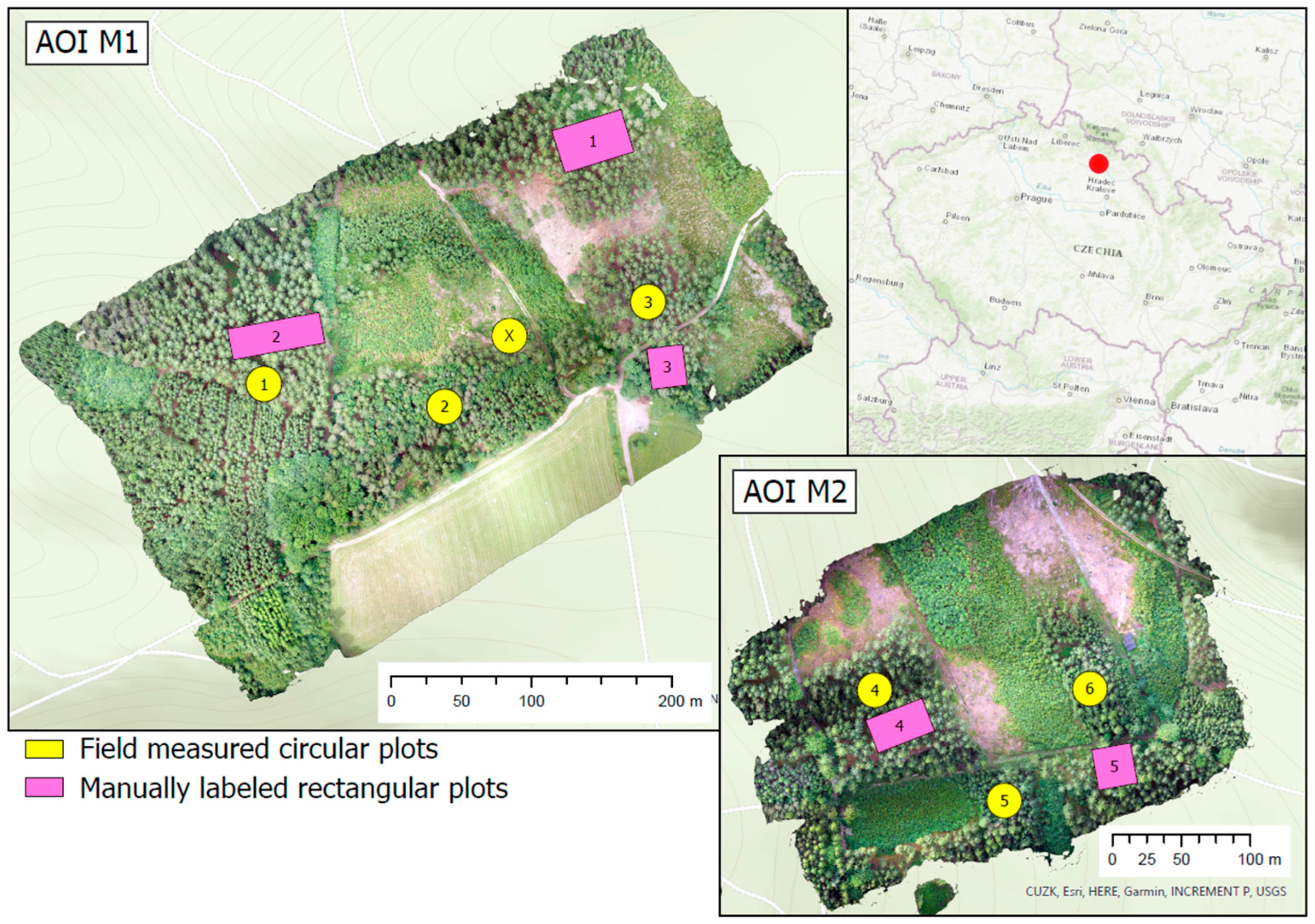
2.1. Study Areas
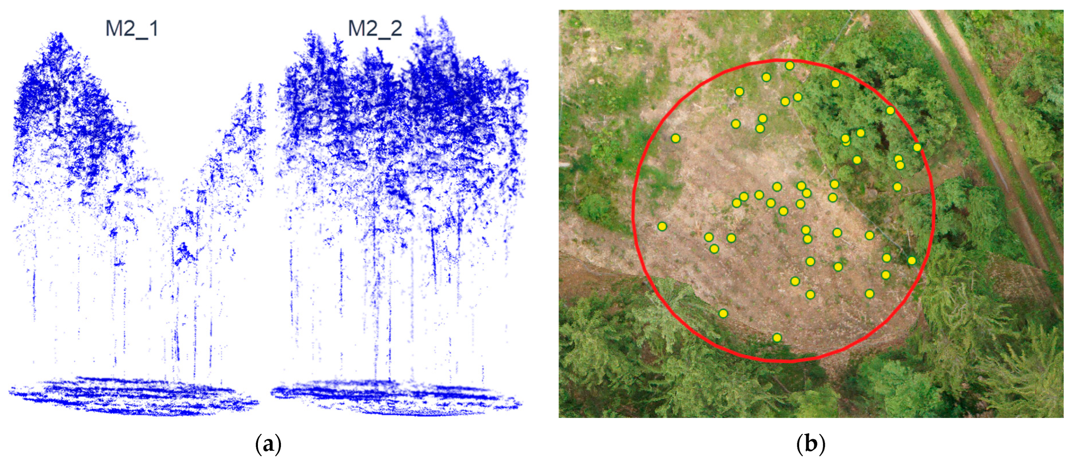
2.2. Data Preprocessing
2.3. Validation Datasets
2.3.1. Field Measurement
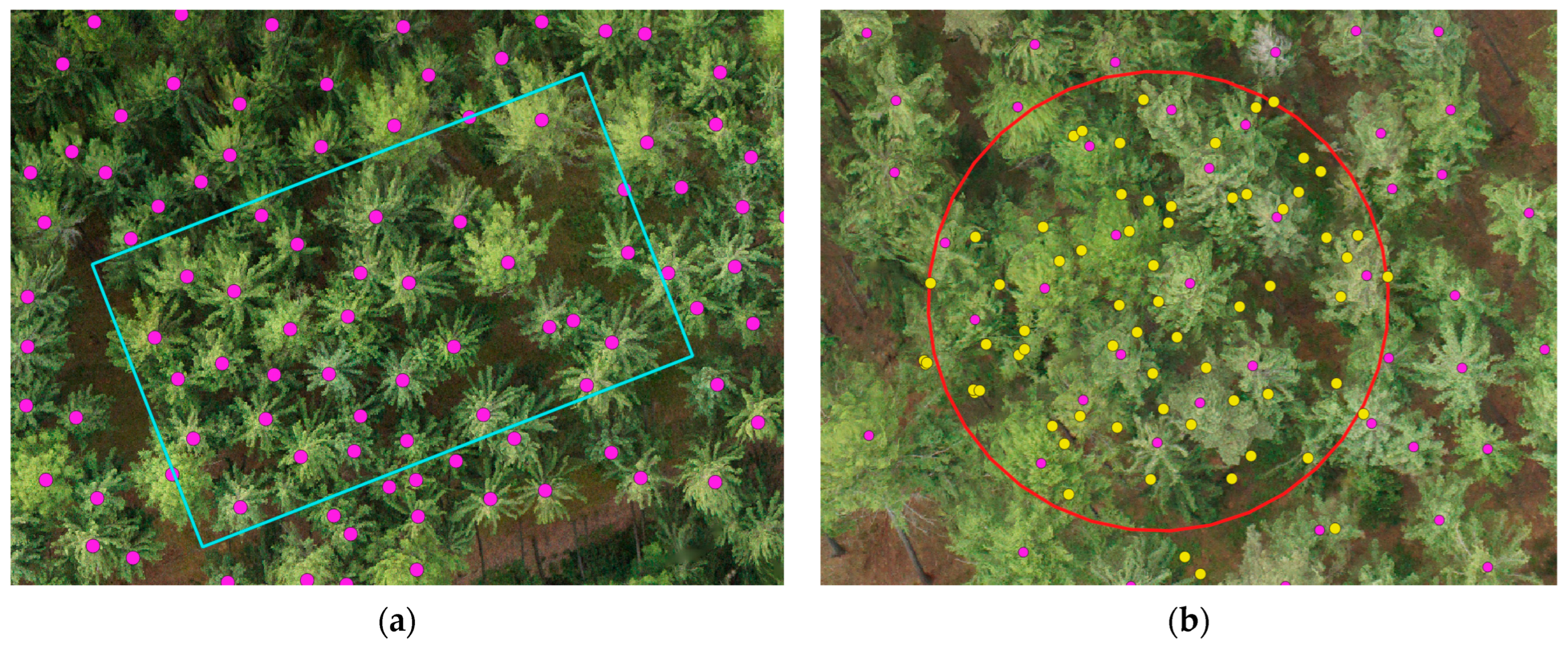
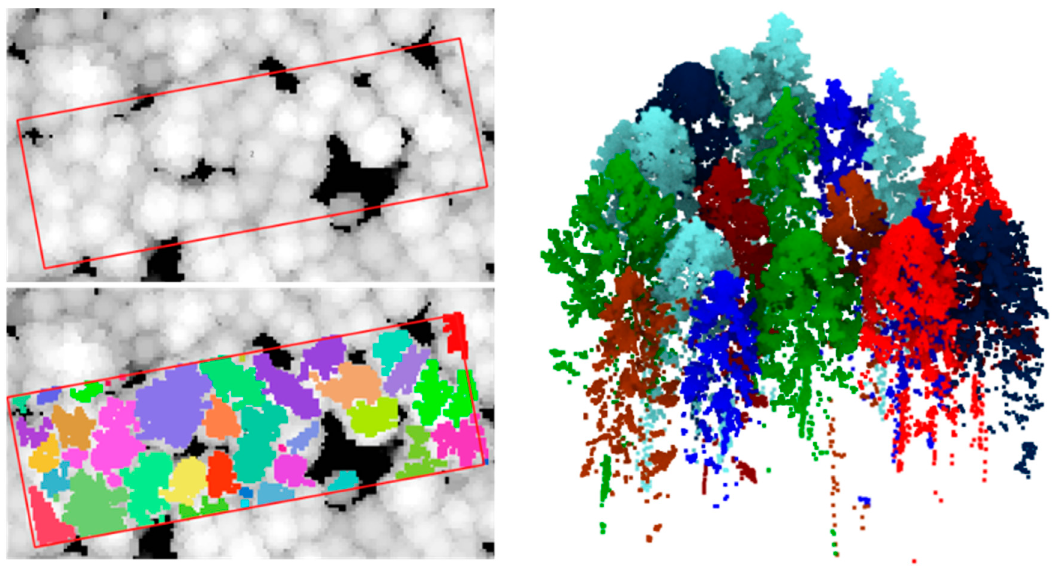
2.3.2. Orthophoto Labels
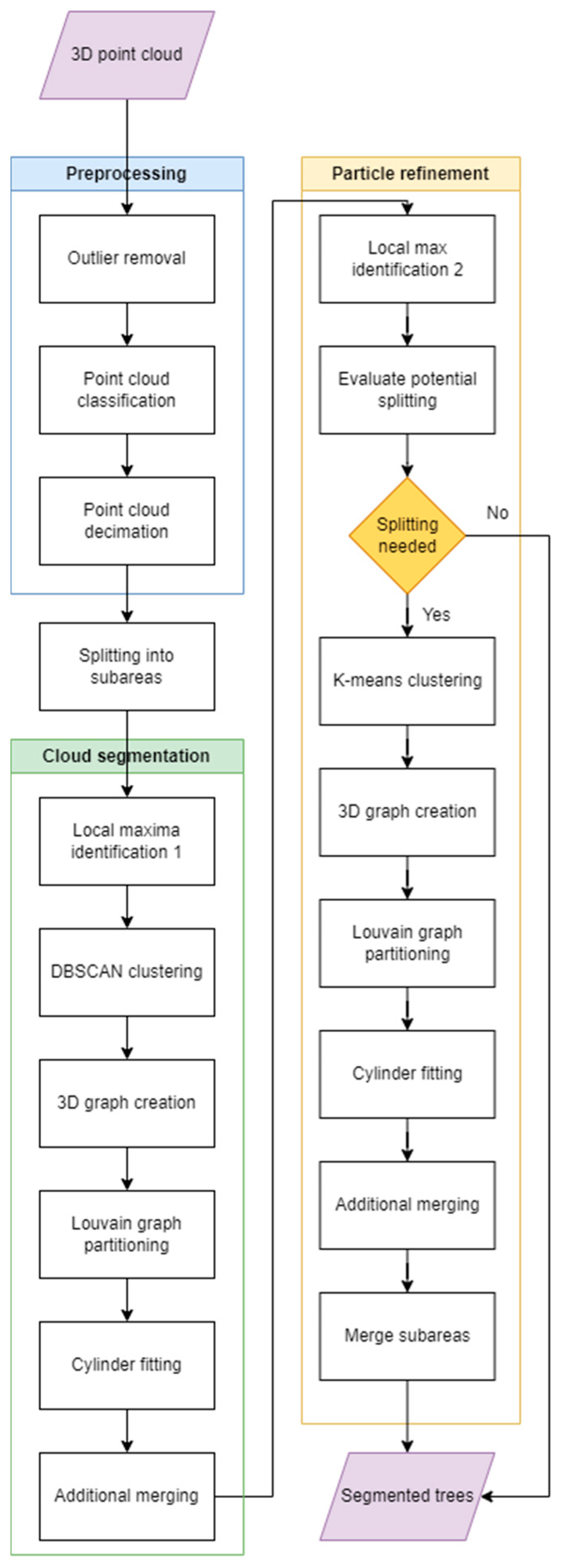
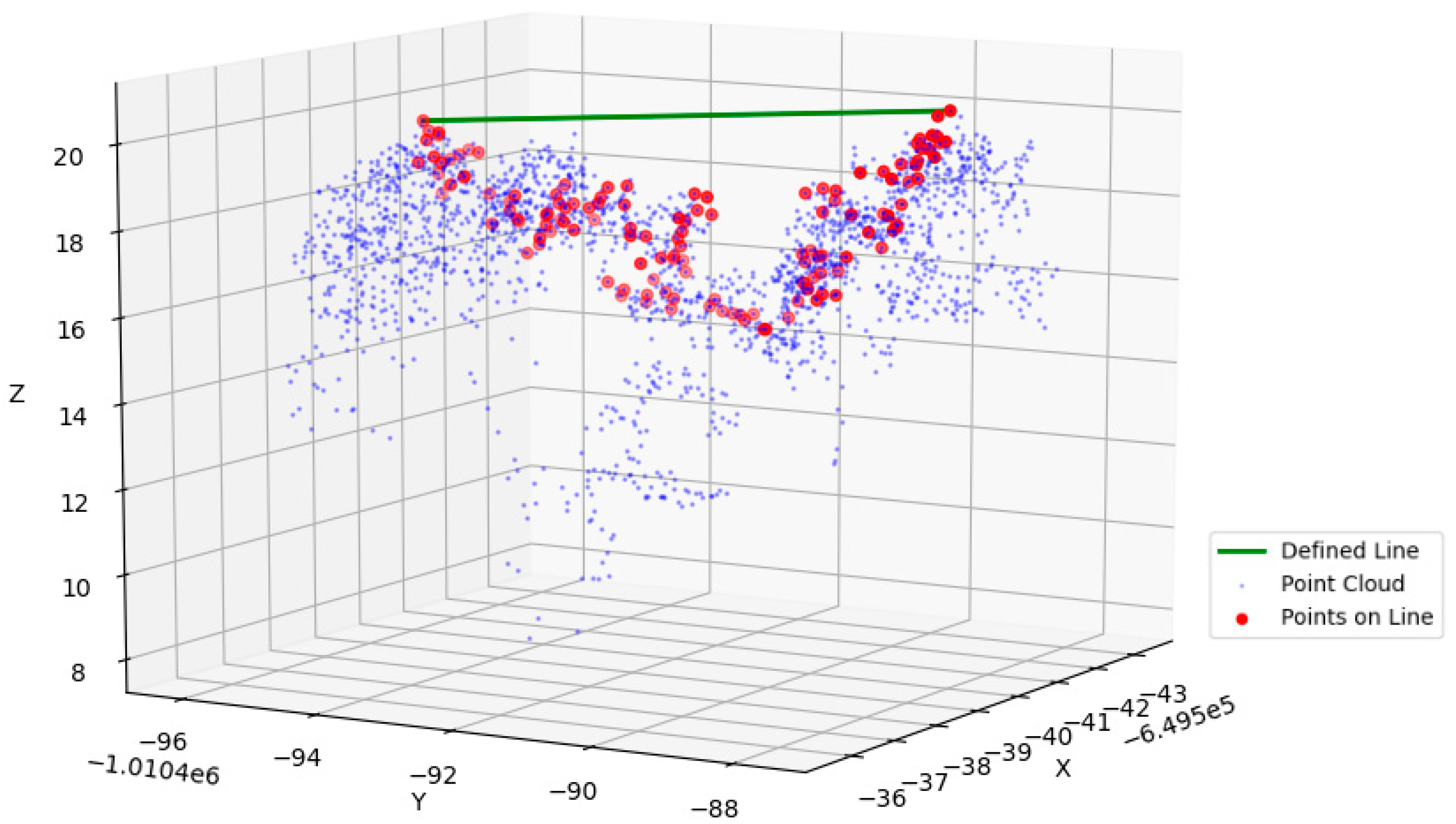
2.4. Method Description
- Preprocessing
- Cloud segmentation
- Particle refinement
- Numpy 1.22.3 (https://numpy.org/, accessed on 6 March 2024);
- Laspy 2.3.0 (https://laspy.readthedocs.io/, accessed on 6 March 2024);
- GDAL 3.5.1 (https://gdal.org/, accessed on 6 March 2024);
- Shapely 1.8.2 (https://shapely.readthedocs.io/, accessed on 6 March 2024);
- PDAL 3.1.2 (https://pdal.io/en/latest/, accessed on 6 March 2024);
- NetworkX 2.8.4 (https://networkx.org, accessed on 6 March 2024);
- SciPy 1.7.3 (https://scipy.org, accessed on 6 March 2024);
- scikit-learn (https://scikit-learn.org, accessed on 6 March 2024);
- scikit-learn (https://scikit-learn.org, accessed on 6 March 2024).
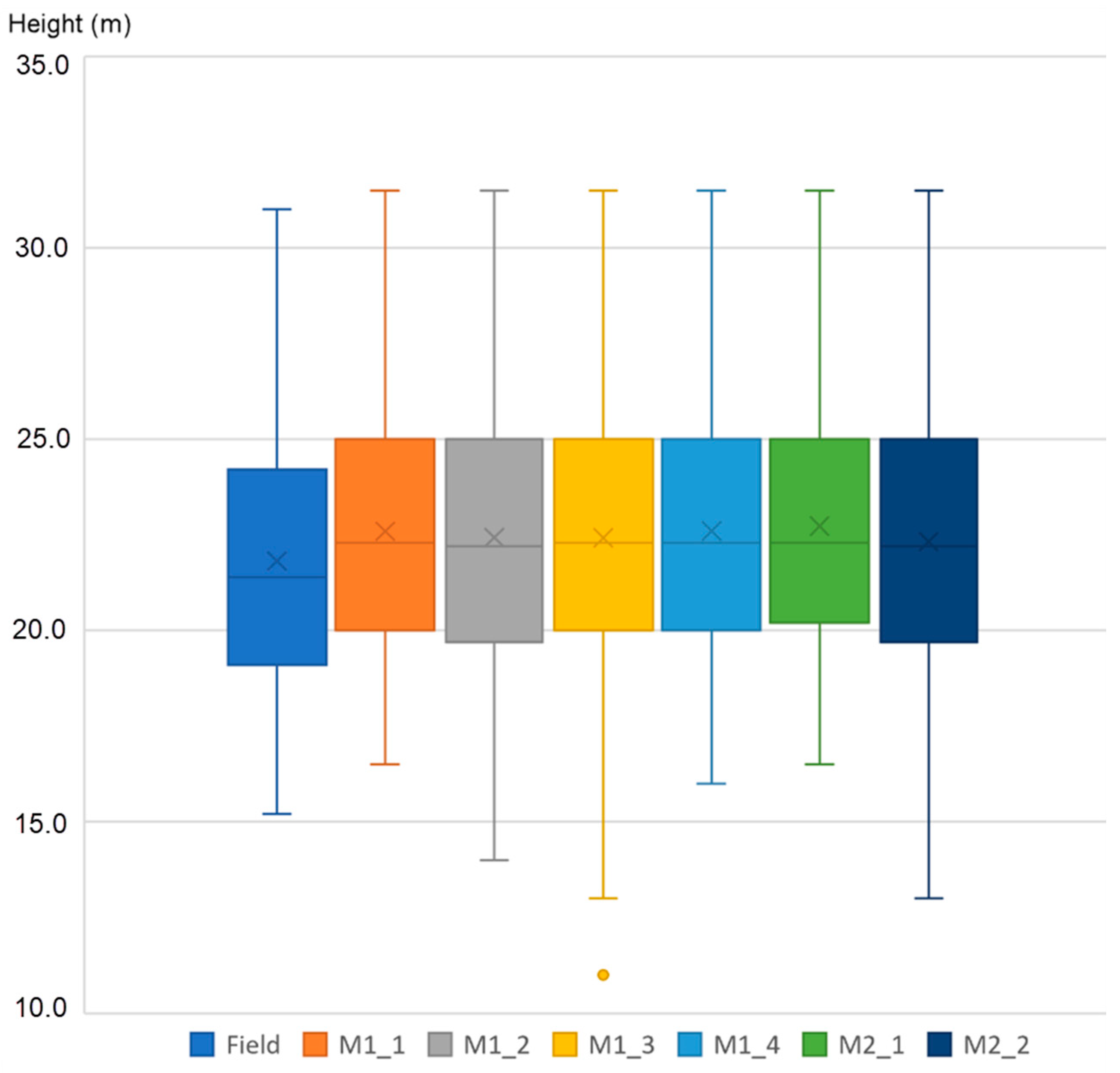
3. Results
- True Positive (TP)—number of correctly segmented trees;
- False Positive (FP)—number segments covering multiple tree labels + number of segments without any tree label;
- False Negative (FN)—the tree label is not covered by any segment area.
4. Discussion
5. Conclusions
Author Contributions
Funding
Data Availability Statement
Conflicts of Interest
References
- Lu, X.; Hu, Y.; Trepte, C.; Zeng, S.; Churnside, J.H. Ocean subsurface studies with the CALIPSO spaceborne lidar. J. Geophys. Res. Ocean. 2014, 119, 4305–4317. [Google Scholar] [CrossRef]
- Chand, D.; Anderson, T.L.; Wood, R.; Charlson, R.J.; Hu, Y.; Liu, Z.; Vaughan, M. Quantifying above-cloud aerosol using spaceborne lidar for improved understanding of cloudy-sky direct climate forcing. J. Geophys. Res. Atmos. 2008, 113, 14. [Google Scholar] [CrossRef]
- Behrenfeld, M.J.; Hu, Y.; Hostetler, C.A.; Dall’Olmo, G.; Rodier, S.D.; Hair, J.W.; Trepte, C.R. Space-based lidar measurements of global ocean carbon stocks. Geophys. Res. Lett. 2013, 40, 4355–4360. [Google Scholar] [CrossRef]
- Winker, D.M.; Pelon, J.R.; McCormick, M.P. CALIPSO mission: Spaceborne lidar for observation of aerosols and clouds. In Lidar Remote Sensing for Industry and Environment Monitoring III; SPIE: online, 2003; pp. 1–11. Available online: https://www.spiedigitallibrary.org/conference-proceedings-of-spie/4881/1/CALIPSO--global-aerosol-and-cloud-observations-from-lidar-and/10.1117/12.462519.short#_=_ (accessed on 6 March 2024).
- Cha, G.; Park, S.; Oh, T. A terrestrial LiDAR-based detection of shape deformation for maintenance of bridge structures. J. Constr. Eng. Manag. 2019, 145, 04019075. [Google Scholar] [CrossRef]
- Buckley, S.J.; Howell, J.A.; Enge, H.D.; Kurz, T.H. Terrestrial laser scanning in geology: Data acquisition, processing and accuracy considerations. J. Geol. Soc. 2008, 165, 625–638. [Google Scholar] [CrossRef]
- Fisher, C.T.; Cohen, A.S.; Fernández-Diaz, J.C.; Leisz, S.J. The application of airborne mapping LiDAR for the documentation of ancient cities and regions in tropical regions. Quat. Int. 2017, 448, 129–138. [Google Scholar] [CrossRef]
- Yu, B.; Liu, H.; Wu, J.; Hu, Y.; Zhang, L. Automated derivation of urban building density information using airborne LiDAR data and object-based method. Landsc. Urban Plan. 2010, 98, 210–219. [Google Scholar] [CrossRef]
- Dubayah, R.O.; Drake, J.B. Lidar remote sensing for forestry. J. For. 2000, 98, 44–46. [Google Scholar] [CrossRef]
- Mazlan, S.M.; Wan Mohd Jaafar, W.S.; Muhmad Kamarulzaman, A.M.; Saad, S.N.M.; Mohd Ghazali, N.; Adrah, E.; Abdul Maulud, K.N.; Omar, H.; Teh, Y.A.; Dzulkifli, D.; et al. A Review on the Use of LiDAR Remote Sensing for Forest Landscape Restoration. In Concepts and Applications of Remote Sensing in Forestry; Springer: Berlin/Heidelberg, Germany, 2023; pp. 49–74. [Google Scholar]
- Gleason, C.J.; Im, J. Forest biomass estimation from airborne LiDAR data using machine learning approaches. Remote Sens. Environ. 2012, 125, 80–91. [Google Scholar] [CrossRef]
- Mascaro, J.; Detto, M.; Asner, G.P.; Muller-Landau, H.C. Evaluating uncertainty in mapping forest carbon with airborne LiDAR. Remote Sens. Environ. 2011, 115, 3770–3774. [Google Scholar] [CrossRef]
- Lovell, J.L.; Jupp, D.L.; Culvenor, D.S.; Coops, N.C. Using airborne and ground-based ranging lidar to measure canopy structure in Australian forests. Can. J. Remote Sens. 2003, 29, 607–622. [Google Scholar] [CrossRef]
- Vincent, L.; Soille, P. Watersheds in digital spaces: An efficient algorithm based on immersion simulations. IEEE Trans. Pattern Anal. Mach. Intell. 1991, 13, 583–598. [Google Scholar] [CrossRef]
- Wu, B.; Wang, Z.; Zhang, Q.; Shen, N.; Liu, J. Evaluating and modelling splash detachment capacity based on laboratory experiments. CATENA 2019, 176, 189–196. [Google Scholar] [CrossRef]
- Hyyppä, J.; Kelle, O.; Lehikoinen, M.; Inkinen, M. A segmentation-based method to retrieve stem volume estimates from 3-D tree height models produced by laser scanners. IEEE Trans. Geosci. Remote Sens. 2001, 39, 969–975. [Google Scholar] [CrossRef]
- Popescu, S.C.; Wynne, R.H.; Nelson, R.F. Measuring individual tree crown diameter with lidar and assessing its influence on estimating forest volume and biomass. Can. J. Remote Sens. 2003, 29, 564–577. [Google Scholar] [CrossRef]
- Cao, L.; Gao, S.; Li, P.; Yun, T.; Shen, X.; Ruan, H. Aboveground biomass estimation of individual trees in a coastal planted forest using full-waveform airborne laser scanning data. Remote Sens. 2016, 8, 729. [Google Scholar] [CrossRef]
- Dalponte, M.; Coomes, D.A. Tree-centric mapping of forest carbon density from airborne laser scanning and hyperspectral data. Methods Ecol. Evol. 2016, 7, 1236–1245. [Google Scholar] [CrossRef] [PubMed]
- Hu, T.; Sun, X.; Su, Y.; Guan, H.; Sun, Q.; Kelly, M.; Guo, Q. Development and Performance Evaluation of a Very Low-Cost UAV-Lidar System for Forestry Applications. Remote Sens. 2020, 13, 77. [Google Scholar] [CrossRef]
- Strîmbu, V.F.; Strîmbu, B.M. A graph-based segmentation algorithm for tree crown extraction using airborne LiDAR data. ISPRS J. Photogramm. Remote Sens. 2015, 104, 30–43. [Google Scholar] [CrossRef]
- Zhang, L.; Li, Z.; Li, A.; Liu, F. Large-scale urban point cloud labeling and reconstruction. ISPRS J. Photogramm. Remote Sens. 2018, 138, 86–100. [Google Scholar] [CrossRef]
- Boulch, A.; Guerry, J.; Le Saux, B.; Audebert, N. SnapNet: 3D point cloud semantic labeling with 2D deep segmentation networks. Comput. Graph. 2018, 71, 189–198. [Google Scholar] [CrossRef]
- Tchapmi, L.; Choy, C.; Armeni, I.; Gwak, J.; Savarese, S. Segcloud: Semantic segmentation of 3d point clouds. In Proceedings of the 2017 International Conference on 3D Vision (3DV), Qingdao, China, 10–12 October 2017; pp. 537–547. [Google Scholar]
- Qi, C.R.; Su, H.; Mo, K.; Guibas, L.J. Pointnet: Deep learning on point sets for 3d classification and segmentation. In Proceedings of the IEEE Conference on Computer Vision and Pattern Recognition, Honolulu, HI, USA, 21–26 July 2017; pp. 652–660. [Google Scholar]
- Liu, Y.; You, H.; Tang, X.; You, Q.; Huang, Y.; Chen, J. Study on Individual Tree Segmentation of Different Tree Species Using Different Segmentation Algorithms Based on 3D UAV Data. Forests 2023, 14, 1327. [Google Scholar] [CrossRef]
- Ullman, S. The interpretation of structure from motion. Proc. R. Soc. Lond. Ser. B Biol. Sci. 1997, 203, 405–426. [Google Scholar] [CrossRef]
- Snavely, N.; Seitz, S.M.; Szeliski, R. Skeletal graphs for efficient structure from motion. In Proceedings of the 2008 IEEE Conference on Computer Vision and Pattern Recognition, Anchorage, AK, USA, 23–28 June 2008. [Google Scholar] [CrossRef]
- Brostow, G.J.; Shotton, J.; Fauqueur, J.; Cipolla, R. Segmentation and Recognition Using Structure from Motion Point Clouds. In Proceedings of the 10th European Conference on Computer Vision: Part I, Marseille, France, 12–18 October 2008; pp. 44–57. [Google Scholar] [CrossRef]
- Rusu, R.B.; Marton, Z.C.; Blodow, N.; Beetz, M. Learning informative point classes for the acquisition of object model maps. In Proceedings of the 2008 10th International Conference on Control, Automation, Robotics and Vision, Hanoi, Vietnam, 17–20 December 2008; pp. 643–650. [Google Scholar]
- Zhang, W.; Qi, J.; Wan, P.; Wang, H.; Xie, D.; Wang, X.; Yan, G. An easy-to-use airborne LiDAR data filtering method based on cloth simulation. Remote Sens. 2016, 8, 501. [Google Scholar] [CrossRef]
- Ester, M.; Kriegel, H.P.; Sander, J.; Xu, X. A density-based algorithm for discovering clusters in large spatial databases with noise. In Proceedings of the KDD96: Proceedings of the Second International Conference on Knowledge Discovery and Data Mining, Portland, OR, USA, 2–4 August 1996; Volume 34, pp. 226–231. [Google Scholar]
- Kriegel, H.-P.; Kröger, P.; Sander, J.; Zimek, A. Density-based clustering. WIREs Data Min. Knowl. Discov. 2011, 1, 231–240. [Google Scholar] [CrossRef]
- Schubert, E.; Sander, J.; Ester, M.; Kriegel, H.P.; Xu, X. DBSCAN revisited, revisited: Why and how you should (still) use DBSCAN. ACM Trans. Database Syst. 2017, 42, 1–21. [Google Scholar] [CrossRef]
- Newman, M.E.J.; Girvan, M. Finding and evaluating community structure in networks. Phys. Rev. E 2004, 69, 026113. [Google Scholar] [CrossRef]
- Blondel, V.D.; Guillaume, J.-L.; Lambiotte, R.; Lefebvre, E. Fast unfolding of communities in large networks. J. Stat. Mech. Theory Exp. 2008, 10, P10008. [Google Scholar] [CrossRef]
- Lancichinetti, A.; Fortunato, S. Community detection algorithms: A comparative analysis. Phys. Rev. E 2009, 80, 056117. [Google Scholar] [CrossRef]
- Traag, V.A.; Waltman, L.; Van Eck, N.J. From Louvain to Leiden: Guaranteeing well-connected communities. Sci. Rep. 2019, 9, 5233. [Google Scholar] [CrossRef]
- Dersch, S.; Heurich, M.; Krueger, N.; Krzystek, P. Combining graph-cut clustering with object-based stem detection for tree segmentation in highly dense airborne lidar point clouds. ISPRS J. Photogramm. Remote Sens. 2021, 172, 207–222. [Google Scholar] [CrossRef]
- Yu, J.; Lei, L.; Li, Z. Individual Tree Segmentation Based on Seed Points Detected by an Adaptive Crown Shaped Algorithm Using UAV-LiDAR Data. Remote Sens. 2024, 16, 825. [Google Scholar] [CrossRef]
- Neuville, R.; Bates, J.S.; Jonard, F. Estimating forest structure from UAV-mounted LiDAR point cloud using machine learning. Remote Sens. 2021, 13, 352. [Google Scholar] [CrossRef]

| Flight ID | Height (m) | Scan Angle (°) | Speed of Flight (m/s) | Scanning Line Dist. (m) | Scan Line Approx. Overlap Min/Max (%) | Scan Line Width (m) | Mean Point Density (Planned) (p/m2) |
|---|---|---|---|---|---|---|---|
| M1_1 | 90 | 60 | 2.0 | 0.10 | 30/20 | 104 | 80 |
| M1_2 | 90 | 60 | 2.7 | 0.13 | 30/20 | 104 | 59 |
| M1_3 | 90 | 90 | 2.0 | 0.10 | 33/25 | 180 | 69 |
| M1_4 | 110 | 60 | 2.0 | 0.10 | 43/37 | 127 | 65 |
| M2_1 | 90 | 60 | 2.0 | 0.10 | 30/16 | 104 | 80 |
| M2_2 | 90 | 90 | 2.0 | 0.10 | 33/20 | 180 | 69 |
| AOI M1 | AOI M2 | |||||||||
|---|---|---|---|---|---|---|---|---|---|---|
| S_plot1 | S_plot2 | S_plot3 | C_plot1 | C_plot2 | C_plot3 | S_plot4 | S_plot5 | C_plot5 | C_plot6 | |
| Area (m2) | 1630 | 1510 | 750 | 490 | 490 | 490 | 840 | 1100 | 490 | 490 |
| CHM mean (m) | 24.5 | 26.3 | 21.8 | 26.5 | 21.3 | 22.6 | 28.3 | 25.1 | 20.5 | 25.8 |
| ML (count) | 47 | 40 | 19 | 14 | 28 | 17 | 36 | 24 | 18 | 48 |
| FL all (count) | X | X | X | 52 | 29 | 56 | X | X | 82 | 101 |
| FL (count) | X | X | X | 17 | 29 | 15 | X | X | 18 | 51 |
| Rectangle Plots | Circular Plots | All Plots | |||||||
|---|---|---|---|---|---|---|---|---|---|
| R (%) | P (%) | F1 (%) | R (%) | P (%) | F1 (%) | R (%) | P (%) | F1 (%) | |
| M1_1 | 91.9 | 84.0 | 87.7 | 89.7 | 86.2 | 88.0 | 91.1 | 84.8 | 87.8 |
| M1_2 | 89.5 | 81.9 | 85.6 | 91.3 | 76.4 | 83.2 | 90.2 | 79.8 | 84.7 |
| M1_3 | 97.0 | 91.4 | 94.1 | 86.3 | 76.0 | 80.1 | 94.7 | 86.5 | 90.0 |
| M1_4 | 98.9 | 93.2 | 96.0 | 93.8 | 80.6 | 86.7 | 97.2 | 88.5 | 92.6 |
| M2_1 | 100 | 93.3 | 96.5 | 91.1 | 77.3 | 83.6 | 95.5 | 84.9 | 89.9 |
| M2_2 | 92.9 | 85.4 | 89.1 | 97.7 | 60.5 | 74.8 | 95.0 | 72.1 | 82.1 |
| Rectangle Plots (OA%) | Circular Plots (OA%) | All Plots (OA%) | ||||
|---|---|---|---|---|---|---|
| Lis Pro 3D | Proposed | Lis Pro 3D | Proposed | Lis Pro 3D | Proposed | |
| M1_4 | 80.5 | 88.8 | 67.2 | 83.8 | 73.9 | 86.3 |
| M2_1 | 76.0 | 86.4 | 41.7 | 80.5 | 58.9 | 83.5 |
Disclaimer/Publisher’s Note: The statements, opinions and data contained in all publications are solely those of the individual author(s) and contributor(s) and not of MDPI and/or the editor(s). MDPI and/or the editor(s) disclaim responsibility for any injury to people or property resulting from any ideas, methods, instructions or products referred to in the content. |
© 2024 by the authors. Licensee MDPI, Basel, Switzerland. This article is an open access article distributed under the terms and conditions of the Creative Commons Attribution (CC BY) license (https://creativecommons.org/licenses/by/4.0/).
Share and Cite
Seidl, J.; Kačmařík, M.; Klimánek, M. A Tree Segmentation Algorithm for Airborne Light Detection and Ranging Data Based on Graph Theory and Clustering. Forests 2024, 15, 1111. https://doi.org/10.3390/f15071111
Seidl J, Kačmařík M, Klimánek M. A Tree Segmentation Algorithm for Airborne Light Detection and Ranging Data Based on Graph Theory and Clustering. Forests. 2024; 15(7):1111. https://doi.org/10.3390/f15071111
Chicago/Turabian StyleSeidl, Jakub, Michal Kačmařík, and Martin Klimánek. 2024. "A Tree Segmentation Algorithm for Airborne Light Detection and Ranging Data Based on Graph Theory and Clustering" Forests 15, no. 7: 1111. https://doi.org/10.3390/f15071111
APA StyleSeidl, J., Kačmařík, M., & Klimánek, M. (2024). A Tree Segmentation Algorithm for Airborne Light Detection and Ranging Data Based on Graph Theory and Clustering. Forests, 15(7), 1111. https://doi.org/10.3390/f15071111