Geospatial Analysis of Relief Degree of Land Surface in the Forest-Steppe Ecotone in Northern China

Abstract

The Relief Degree of Land Surface (RDLS) is an important index to evaluate regional environment. It has a significant effect on the local climate, geologic hazards, the path and speed of fire spreading, the migrations of wild animals, and the runoff path and speed of precipitation. The forest-steppe ecotone in northern China is one of ecological fragile zones. In-depth study of the RDLS of the forest-steppe ecotone in northern China will help to implement ecological projects scientifically and promote the construction of the national ecological security barrier. The Shuttle Radar Topography Mission (SRTM-GL1 30 m) data were used to determine the optimal analysis window for RDLS based on the mean change-point method, and the elevation difference was extracted based on the window analysis method. The RDLS model was used to extract RDLS of the forest-steppe ecotone and analyzed with the help of a spatial auto-correlation model. The correlation between mean elevation, relative elevation difference, and RDLS was also analyzed. The results show that the optimal analysis window size for RDLS was 29 × 29, corresponding to an area of 0.76 km². The RDLS under the optimal analysis window extracted from SRTM-GL1 (30 m) ranged from 0.084 to 3.516. The RDLS had significant spatial clustering, with high RDLS mainly distributed in the mountainous areas and low RDLS mainly distributed in mountain-to-plain transition zone; the RDLS between different administrative units and different watersheds had obvious variability. Overall, the RDLS was characterized as decreasing, increasing, and then decreasing from the south to north, while it was high in the west and low in the east. And the RDLS was linearly positively correlated with mean elevation and relative elevation difference. In the future, the implementation of major ecological projects in the forest-steppe ecotone in northern China, such as soil and water conservation, afforestation tree species selection, ecological corridor design, ecological management, geological disaster prevention, and forest fire prevention, should fully consider the local topographic conditions. These research results can provide topographic references for the implementation of ecological planning and engineering in this area and similar areas. It contributes to sustainable development and maximization of ecological benefits and promotes the establishment of a national ecological security barrier.

1. Introduction

Topographic relief is a key indicator in the respond to the state of the land surface. It reflects the natural properties of land surface. It also indicates the potential for regional land use. This has a substantial application value in the fields of geography, ecology, resources, and environment. Topographic relief has been widely used in various fields. It is applied in ecological environment evaluation [1] and geohazard research [2,3,4,5]. It is also utilized in urban street network analysis [6] and studies of mountain and landform type analysis [7]. Additionally, it aids in population and settlement distribution studies [8,9,10,11,12] and soil erosion studies [13]. Topographic relief is important in geomorphic spatial pattern analysis [14] and identifying riparian ecological restoration factors [15]. Moreover, it is used to assess the spatial risk of extreme precipitation [16] and spatial pattern of urban- rural integration [17].

Ecologically fragile zones are located in the interlacing regions of different ecosystems [18]. The forest-steppe ecotone is characterized by a diverse mix of grasses, trees, and shrubs [19,20]. The formation of this ecotone is the result of the comprehensive action of regional climate, hydrology and topographic conditions [21,22]. Forest-steppe ecotones are generally distributed in mosaic patterns. Different levels of land use practices, such as mowing and grazing, occur in these ecotones [23,24]. In general, the forest-steppe ecotones exhibit a fragile ecological environment [24]. Additionally, there are pronounced edge effects, and habitat heterogeneity [24].

The forest-steppe ecotone in northern China is an important part of the Eurasian forest-steppe ecotone [23]. In the east, it is situated in the transition area between the Greater Khingan Mountains and the outer margin of the Yanshan Mountains. It is also located in the vicinity of the Northeast Plain. In the west, it marks the junction between the eastern margin of the Inner Mongolia Plateau and the Yanshan Mountains. To the south, it lies in the transitional areas of the Taihang Mountain and Yanshan Mountain ranges [18,25]. In terms of administrative area, it spans from north to south across Hulun Buir City, Xingan League, Tongliao City and Chifeng City of the Inner Mongolia Autonomous Region. It also crosses some counties (banners, cities, and districts) of Chengde City and Zhangjiakou City in Hebei Province. As an important ecological protection barrier in the Northeast Plain, Beijing-Tianjin-Hebei, and the North China Plain, this ecotone plays a vital ecological role. It contributes significantly to windbreak and sand fixation, climate regulation, and soil and water conservation. This ecotone holds an irreplaceable strategic position in maintaining regional ecological security.

However, the forest-steppe ecotone in northern China is also an ecologically fragile area, where the long-term impacts of natural and social factors have led to different degrees of environment degradation. The project of returning farmland to forest and grassland is a significant undertaking in ecological restoration [26,27], which can aid in the regeneration of degraded ecosystems [28]. China has established the goal of achieving carbon neutrality by 2060. The implementation of ecological projects in fragile areas is beneficial to the process of ecological restoration [29,30]. It is also the primary method of increasing soil carbon storage [29,30]. Since 2000, a series of key ecological projects have been conducted in this region [31]. Ecological restoration efforts are significantly influenced by topographic features [32]. Previous studies have shown that topography constrains the availability of nutrients [33] and water for plant growth. It is essential to the structure of mountain forests [34]. Topography plays a pivotal role in the Holocene biome migration [35]. It has a strong impact on the vertical migration of forests in northern China’s forest-steppe ecotone [36]. Additionally, the buffer effect of topographical factors enabled forest ecosystems in the southeastern Inner Mongolia Plateau to survive the Holocene drought events [37].

Therefore, as a geographically unique and important region, topographic research is crucial for the protection and sustainable development of the ecological environment in northern China’s forest-steppe ecotone. It is of practical significance in guiding the promotion of the protection and restoration of natural forests. It can also aid in the scientific implementation of afforestation planning. Additionally, it will enhance the ecological benefits of projects such as wind prevention, sand fixation, and water conservation. Currently, topographic relief studies have only been conducted in other areas [1,38,39,40], and there is a lack of research that is fully consistent with this study area. This study utilized elevation data to investigate the topographic relief of northern China’s forest-steppe ecotone. The analysis was conducted using the window analysis method, mean change-point method, RDLS model, and spatial auto-correlation method. The main objectives were to deepen the understanding of the topographic characteristics of the area and to provide a foundation for soil and water conservation, afforestation tree species selection, ecological corridor design, ecological management, geological disaster prevention, and forest fire prevention. Additionally, the study also aims to promote the scientific implementation of ecological projects in this area and similar areas. This research will contribute to sustainable development and the maximization of ecological benefits and promote the establishment of a national ecological security barrier.

2. Materials and Methods

2.1. Study Area

The forest-steppe ecotone in northern China is situated in the marginal zone of the East Asian summer monsoon [18,41] (Figure 1a,b). It is a semi-humid to semi-arid transition zone in northern China, characterized by dry winds, limited precipitation, and heightened evaporation in spring, leading to susceptibility to spring drought. In summer, the region is controlled by the East Asian monsoon [41], and in winter, it is controlled by strong Mongolian-Siberian high pressure [41], which is cold and dry, with northwesterly or northerly winds prevailing. The temperature in this region decreases from south to north. The temperature difference is large, and the annual average temperature stands at 3.84 °C. The 400 mm precipitation line passes through the region [41,42,43], with precipitation decreasing from southeast to northwest, concentrated in June–August. The primary vegetation types include deciduous broad-leaved forest, mixed coniferous forest, scrub, and sparsely forested grassland [44,45,46]. The vegetation field survey map is shown in Figure 1c. Disregarding systematic errors, the altitude of the study area was determined using the Shuttle Radar Topography Mission (SRTM-GL1 30 m) sourced from the United States Geological Survey (USGS), ranges from 83 to 2849 m, as shown in Figure 1d.

2.2. Data Sources

In this study, we used the SRTM-GL1 datasets to extract the RDLS for the forest-steppe ecotone in northern China. They were sourced from the United States Geological Survey (USGS) (https://earthexplorer.usgs.gov/, accessed on 6 October 2023). The SRTM data product adopts the WGS84 coordinate system as the horizontal reference. The dataset uses a horizontal spatial resolution of 1″ (approximately equivalent to 30 m at the equator) [47,48]. Compared with ASTER GDEM, another 1″ resolution dataset, SRTM-GL1 demonstrates superior overall elevation accuracy [47]. Basic geographic data, namely administrative boundaries at various levels, were sourced from the National Catalogue Service for Geographic Information (https://www.webmap.cn/main.do?method=index, accessed on 27 September 2023).

2.3. Research Method

2.3.1. Window Analysis Method

The window analysis method for raster data involves employing an analysis window with a fixed analysis radius for raster data wherein a sequence of calculations, such as mean value and summation, are performed. In the study, the window analysis method was adopted to extract the relative elevation difference required for the RDLS in the transitional zone between forest and steppe in northern China. Using a rectangular analysis window as the window type, the calculations for the maximum value, minimum value, and relative elevation difference of the pixels under the window n × n (n ≥ 2) were performed (where n indicates window size). Regarding the upper limit of n, signifying the maximum window size to be considered, there is no uniform consensus in the academic community, and researchers typically determine its value based on the conditions of the study area and data accuracy [1,38]. In this study, based on the SRTM-GL1 (30 m) data of northern China’s forest-steppe ecotone, we conducted a window analysis test, determining the window size (n) to be in the 2–90 range.

2.3.2. Mean of Change-Point Method

Previous studies have demonstrated that the topographic relief with window area variation follows a logarithmic curve, and there must be a unique inflection point on the curve from steep to slow [1], that is, the optimal statistical unit. The mean change-point analysis method in statistics proved to be the most effective for this test, with a single variable point [1]. In the study, the mean change-point method was adopted to determine the optimal analysis window for the RDLS, using the prescribed steps [1,38,39,49].

(1) Utilizing the formula: (H) = Max(H) − Min(H), the relative elevation difference was computed under N incremental analysis windows (2 × 2, 3 × 3, …, 90 × 90). Subsequentially, the unit topography relief (T) was calculated using the following formula:

$$T_i=t_i/S_i (i=2, 3, 4, \dots , 90)$$

(1)

where T_i is the unit topography in the ith analysis window, t_i is relative elevation difference, and S_i is the area of the analysis window.

(2) The logarithm (lnT) of the series of unit geopotential degrees (T) obtained from the above calculations resulted in a nonlinear series X_k (k = 2, 3, …, 90).

(3) For each i, the above nonlinear series X_k was divided into two parts: X₂, X₃, …, X_k−1, and X_k, X_k+1, …, X₉₀. The arithmetic means $\overline{X_{k1}}$ and $\overline{X_{k2}}$ of the preceding and following sequences, and the arithmetic mean $\overline{X}$ of the total sample, were calculated respectively.

(4) The corresponding statistics were calculated using Equations (2) and (3):

$$S={\displaystyle \sum _{t=2}^N{\left(X_t-\overline{X}\right)}^2}$$

(2)

$$S_k={\displaystyle \sum _{t=2}^{i-1}{\left(X_t-\overline{X_{k1}}\right)}^2}+{\displaystyle \sum _i^{90}{\left(X_t-\overline{X_{k2}}\right)}^2}$$

(3)

where S represents the sum of the squares of the deviation of the total sample, and S_k is the sum of the squared deviations of the first and last samples.

(5) The value of S − S_k was calculated, where the maximum value S − S_k is considered the optimal analysis window of topographic relief, and the corresponding window area is identified as the optimal statistical unit.

2.3.3. RDLS Model

Most of the existing studies consider topographic relief as the height difference between the highest and lowest points in each zone [5,40], which is easy to understand; however, the calculation is too simple and ignores the relationship among elevation, relative elevation difference, and flat and non-flat land. In this study, the RDLS model, put forward by Feng et al. [50], was adopted to calculate RDLS of northern China’s forest-steppe ecotone based on the relative elevation difference within the optimal window. The model takes into account the effects of elevation, relative height difference, and flat and non-flat areas on topographic relief in a given area [50]. The formula is expressed as below [10,50]:

$$RDLS=ALT/100+\left\{\left[Max\left(H\right)-Min\left(H\right)\right]\times \left[1-P\left(A\right)/A\right]\right\}/500$$

(4)

where RDLS is the Relief Degree of Land Surface; ALT is mean altitude (m) within a specific area centered on a raster cell; Max(H) and Min(H) are the highest and lowest elevations (m) in the region, respectively; P(A) corresponds to the flat land area (km²) in the region, representing the area with the relative elevation difference < 30 m within the optimal window; and A is the total area of study area (km²).

2.3.4. Spatial Autocorrelation Analysis

Spatial autocorrelation is a crucial concept in spatial statistics. It describes the geospatial correlation of the attribute values of a study object. This correlation is influenced by its arrangement or position [51]. It highlights the correlation between the attribute in a spatial reference unit and its neighboring space unit [52,53]. This analysis reveals how attributes relate across geographical space. Commonly used spatial correlation analysis methods include Join count statistics [54,55], Moran’s index (Moran’s I), Ripley’s K [56], Geary’s C, and Getis Ord Gi* [51,52] Among them, Moran’s I is the most commonly utilized [57]. It includes global Moran’s I and local Moran’s I [57]. The former usually indicates whether the attribute values are spatially clustered, while the latter identifies the specific areas where the high or low values cluster [57]. Both of them have been widely used in many research fields [51,58,59,60].

Global Moran’s I

The calculation formula for global Moran’s I is as listed below [60,61]:

$$I=\frac{n{\displaystyle {\sum }_{i=1}^n{\displaystyle {\sum }_{j=1}^n{W}_{ij}\left(X_i-\overline{X}\right)\left(X_j-\overline{X}\right)}}}{{\displaystyle {\sum }_{i=1}^n{\displaystyle {\sum }_{j=1}^n{W}_{ij}{\displaystyle {\sum }_{i=1}^n{\left(X_i-\overline{X}\right)}^2}}}}$$

(5)

where X_i and X_j represent ith and jth variable values, and $\overline{X}$ is the mean of all X. W_ij is the spatial weight between the ith and jth variables, and n is the number of observations.

The I ranges from −1 to 1. When the value of I is greater than 0, it indicates spatial clustering of similar values. Conversely, when I is less than 0, it indicates a spatial dispersion. When the value of I is close to 0, it implies a random spatial pattern. The z-score method was employed to ascertain the significance of global Moran’s I, assuming a random pattern with an average of 0 and a variance of 1 [58]. When the z-score is greater than 0, it implies neighboring features with similar values. Conversely, when the z-score is less than 0, it indicates the neighboring feature have dissimilar values [51,62].

Local Moran’s I

Local spatial autocorrelation is a vital technique for the identification of crash hot and cold spots. Local Moran’s I is a frequently employed statistic in the field of local spatial autocorrelation [62]. The calculation formula of Local Moran’s I is as listed below [61,63]:

$$I_i=\frac{n\left(X_i-\overline{X}\right){\displaystyle {\sum }_{j=1,j\ne i}^n{W}_{ij}\left(X_j-\overline{X}\right)}}{{\displaystyle {\sum }_{i=1}^n{\left(X_i-\overline{X}\right)}^2}}$$

(6)

The parameters are same to global Moran’s I. Local Moran’s I typically includes four clustering patterns: high values cluster together, high value surrounded by low value, low values cluster together, and low value surrounded by high value [62].

3. Results

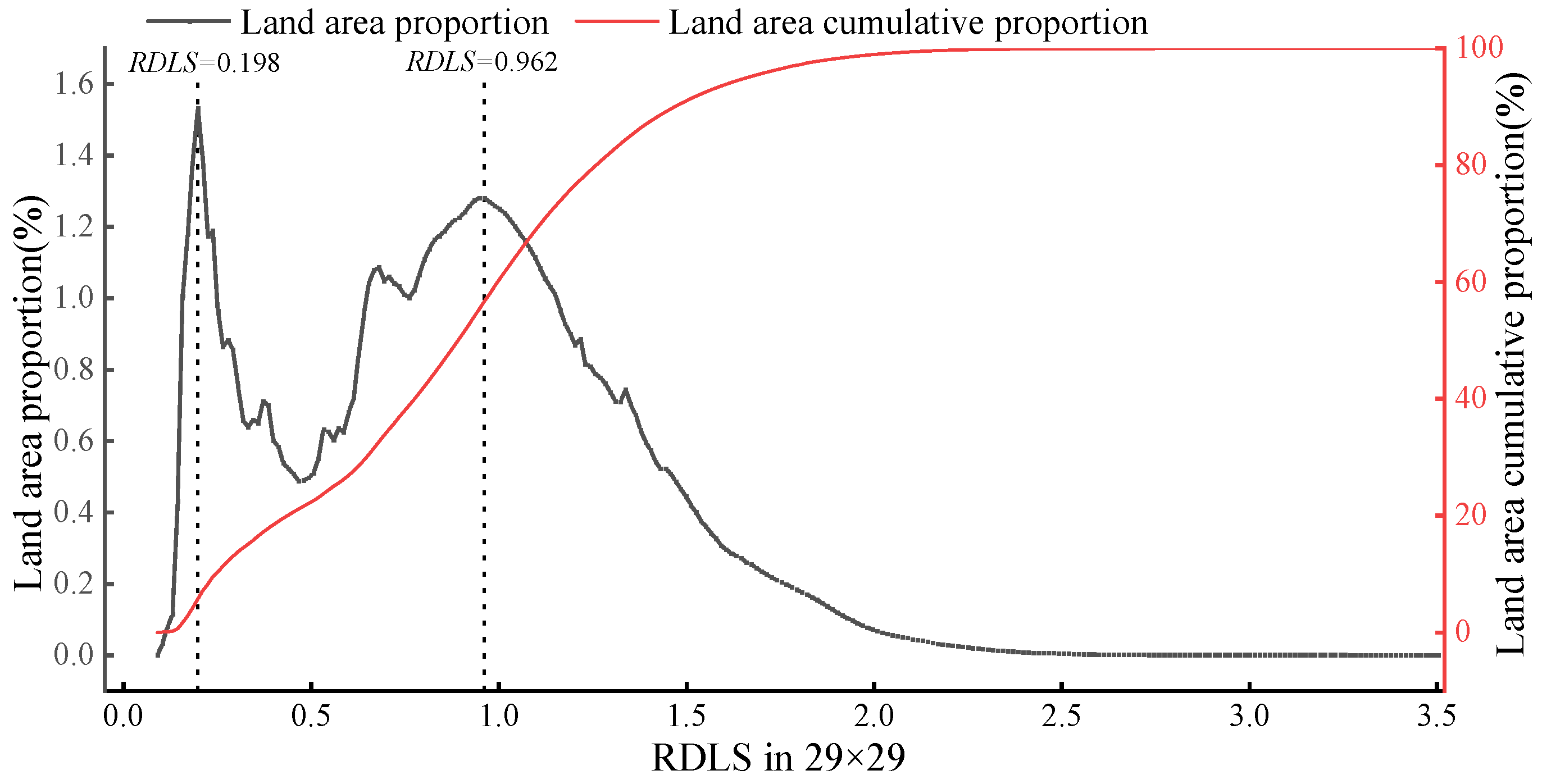
3.1. Distribution of RDLS under Optimal Window

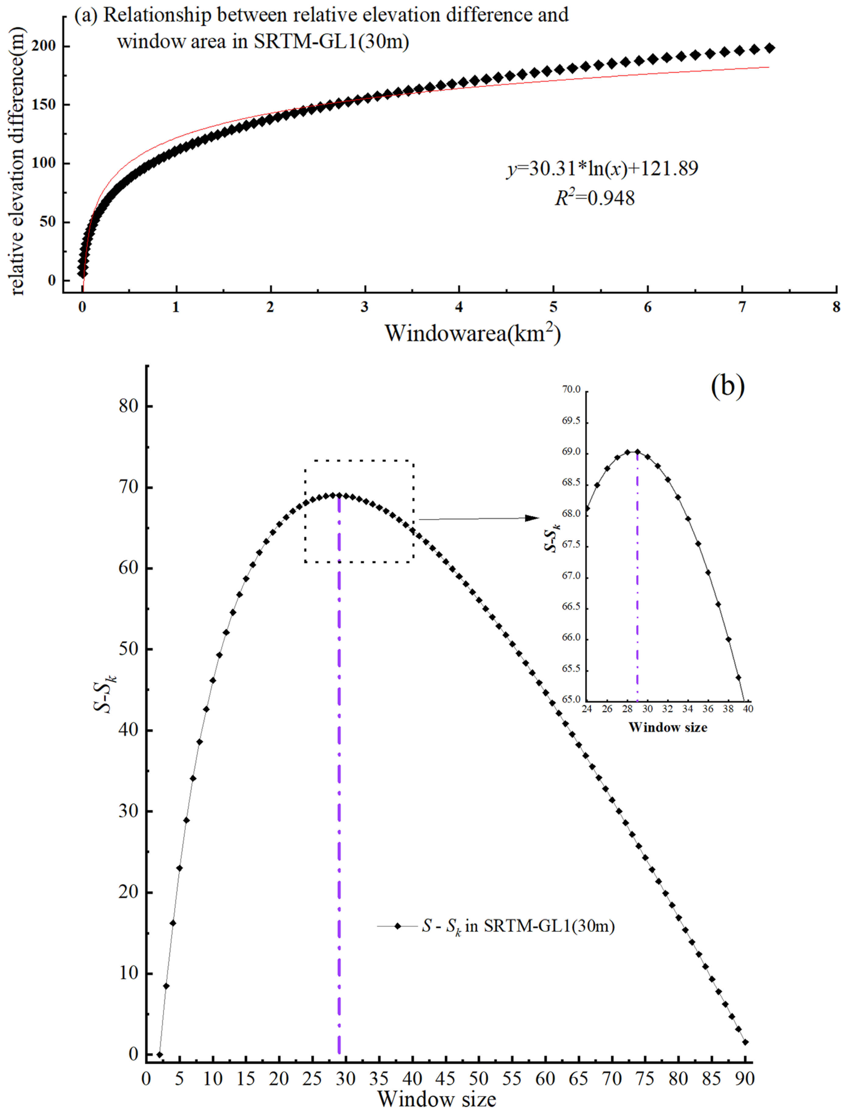
3.1.1. Determination of Optimal Analysis Window for RDLS Based on the Mean of the Change-Point Method

Four window sizes (16 × 16, 35 × 35, 56 × 56, and 78 × 78) were randomly selected to calculate the relative height difference and RDLS of northern China’s forest-steppe ecotone based on SRTM-GL1 (30 m). The relationship between window size and RDLS was analyzed; the result showed that the RDLS extracted from SRTM-GL1 (30 m) increased with the increase of window size (Figure 2 and Figure 3). Furthermore, as the analysis window increased, the region with an RDLS range from 0.084 to 1.076 continued to decrease, whereas the region with an RDLS above 1.076 expanded (Figure 2 and Figure 3). These observations suggest that a larger analysis window corresponds to a larger relative elevation difference. However, a larger analysis window does not mean a more accurate extraction for RDLS. If the window is too large, some details of the RDLS of target mountains may be hidden. In addition, a too-large window will also include information on other mountains except for the target mountains [49]. Therefore, it is crucial to determine the optimal analysis window for calculating the RDLS of this study area.

Scatter plots were generated with the relative elevation difference under different windows of SRTM-GL1 (30 m) as the dependent variable, and the window area was the independent variable (Figure 4a). The logarithmic function emerged as the optimal trend function for the relationship between the window area and the relative elevation difference of SRTM-GL1 (30 m), exhibiting an R² of 0.948 (Figure 4a). According to the change of S − S_k, it can be determined that there was only one “inflection point” where the local height difference changed from a sudden increase to a gentle decrease (Figure 4b), and this point corresponded to the optimal analysis window. The results showed that based on SRTM-GL1 (30 m) data, the optimal analysis window for the RDLS of study area was 29 × 29 (rectangular neighborhood), covering an approximate area of 0.76 km².

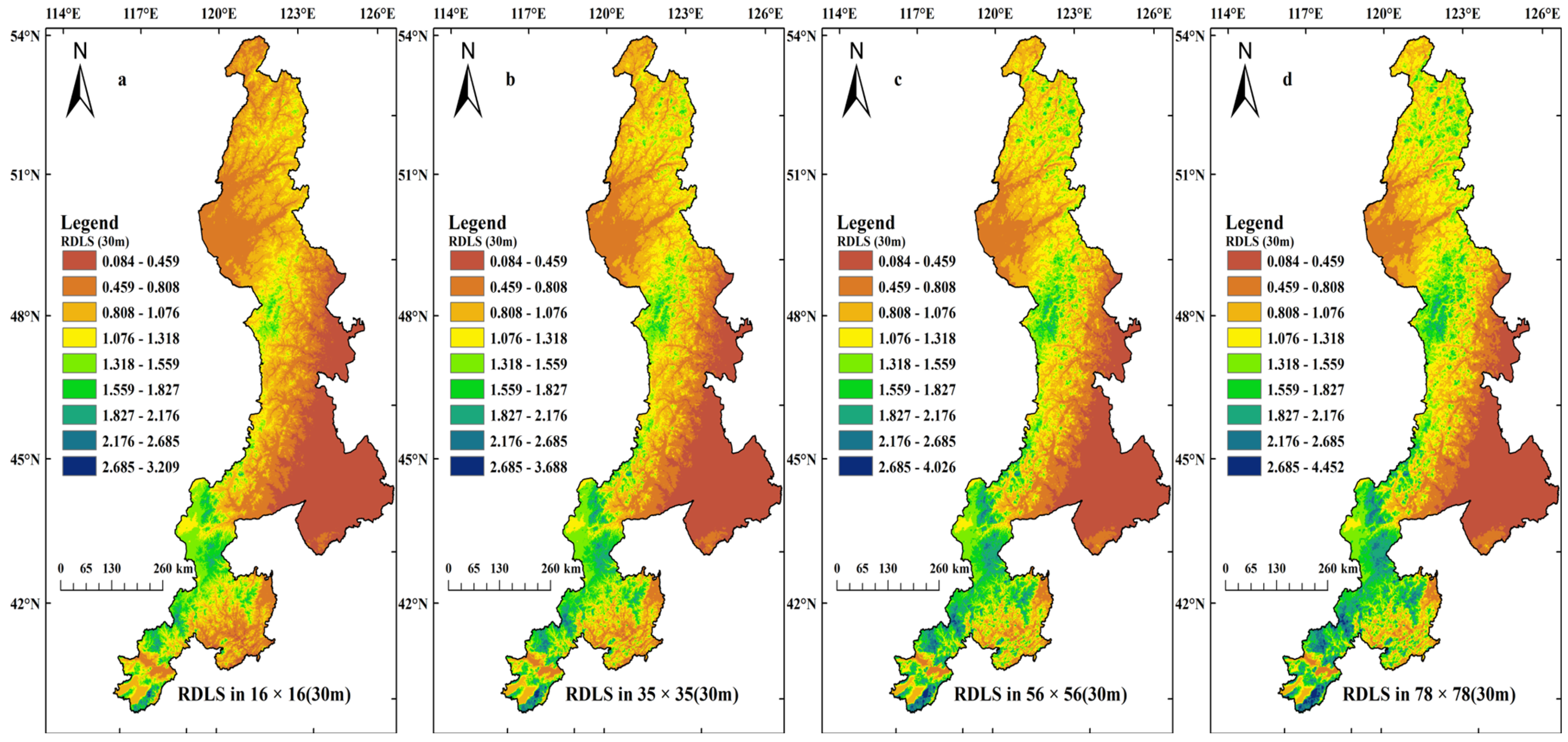
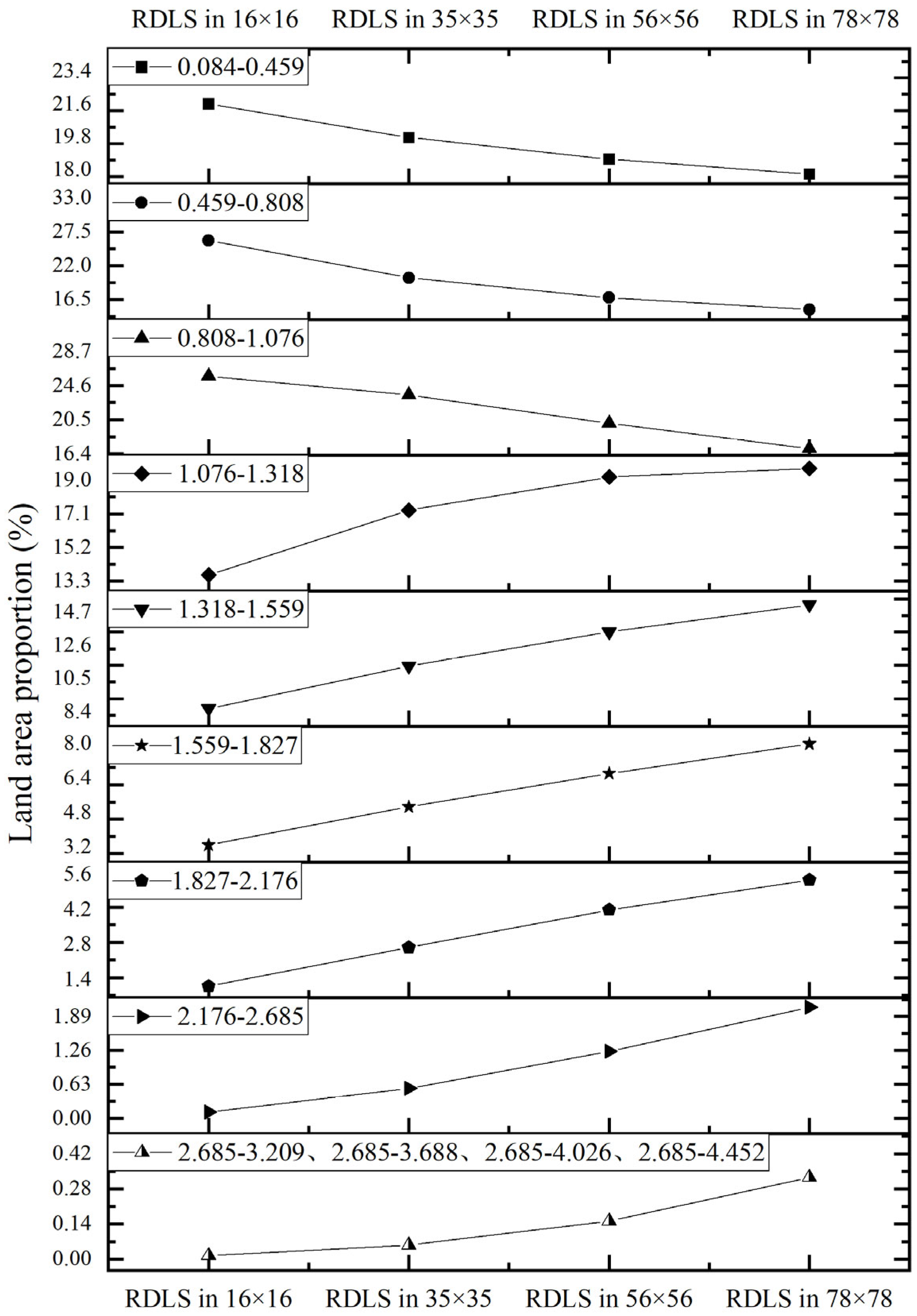
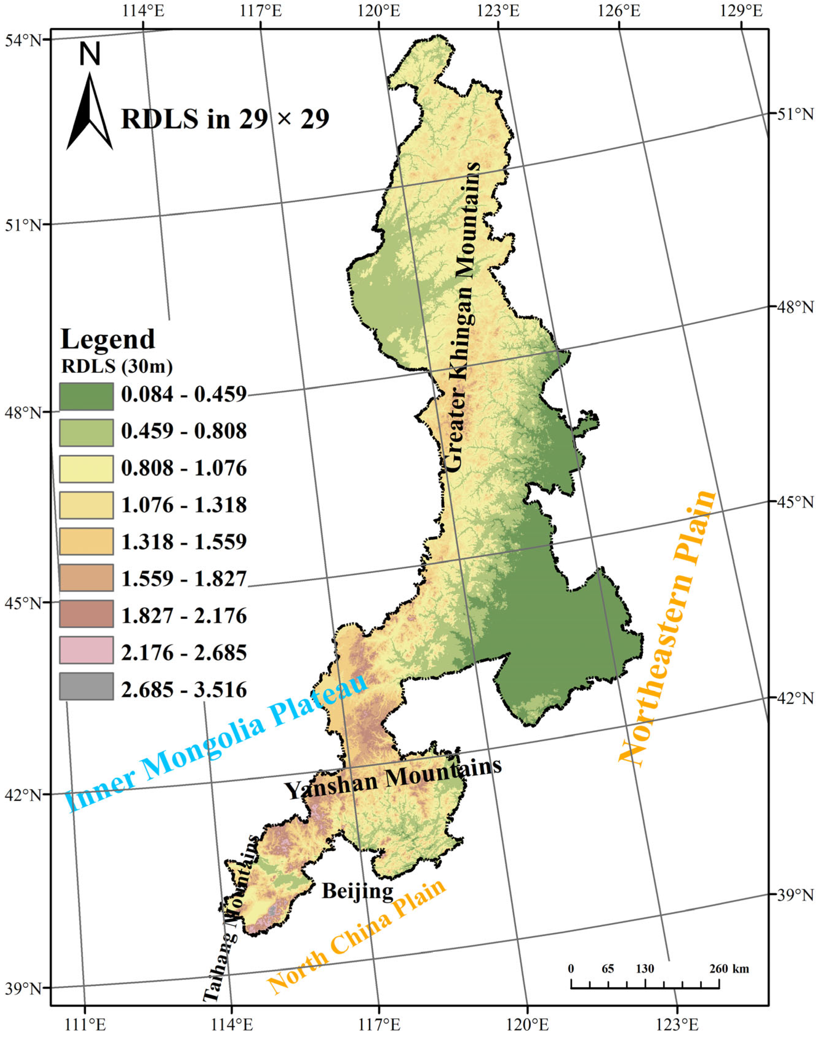
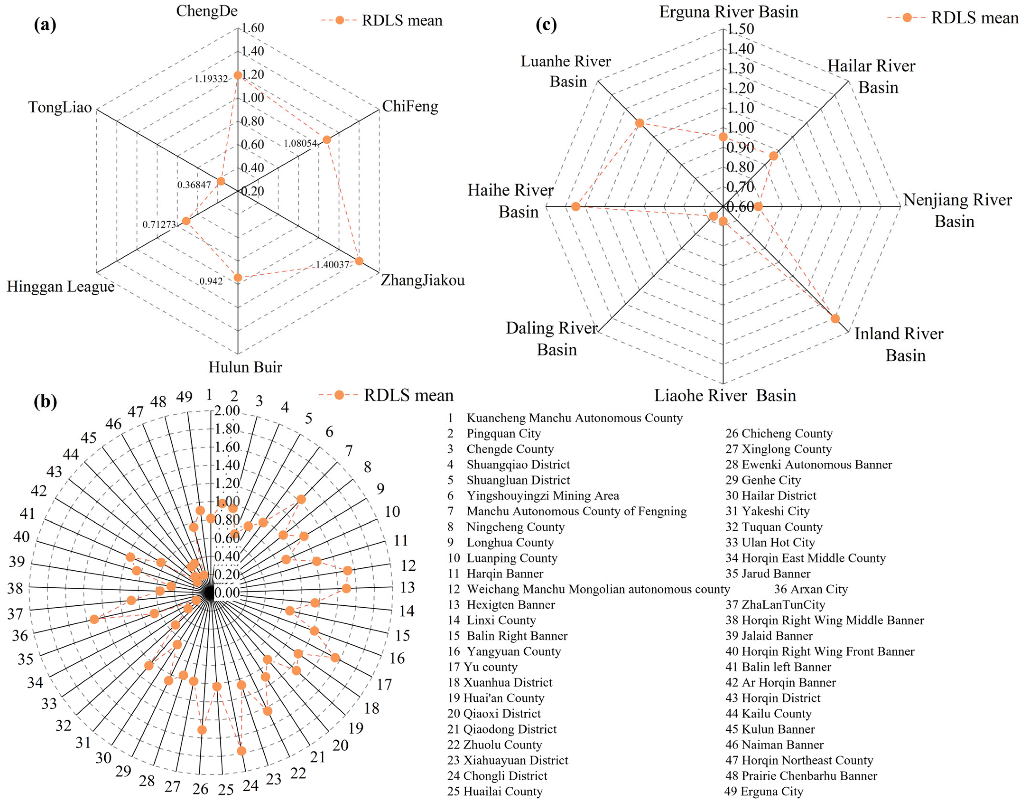
3.1.2. RDLS under the Optimal Analysis Window

Under the optimal window, the RDLS of the study area ranged from 0.084 to 3.516 (Figure 5), with a mean of 0.887. Approximately 98.52% of the area was focused within the range of 0.084–1.934 (Figure 6), with two prominent peaks of the proportion observed at 0.198 and 0.962 (Figure 6). In terms of spatial distribution, high RDLS within the optimal window of northern China’s forest-steppe ecotone were predominantly situated in mountainous areas. These areas included the Yanshan Mountains, encompassing Zhangjiakou City and Chengde City, namely the southern slope of Greater Khingan Mountains south of Hulun Buir City and north of the Hinggan League. Additionally, the eastern edge of the Inner Mongolia Plateau and the northern foot of the Yanshan Mountains west of Chifeng City were part of high-RDLS areas. Conversely, low-RDLS areas were mainly observed in the central and eastern parts of Tongliao City. The eastern part of the Hinggan League, representing the transition area from the Inner Mongolia Plateau and the Greater Khingan Mountains to the Northeast Plain, also had low-RDLS areas. In addition, the low-value area also comprised the transition area from the western side of the Greater Khingan Mountains to the Hulun Buir Grassland (Figure 5).

From the perspective of city scale, Zhangjiakou City had the largest RDLS, with a mean value of 1.40; followed by Chengde City, with a mean value of 1.19; and Tongliao City had the smallest RDLS, with a mean value of 0.37 (Figure 7a). From the perspective of county scale, the RDLS of Chongli District was the largest, with a mean value of 1.77; followed by Yu County (a mean value of 1.54) and Weichang Manchu Mongolian autonomous county (a mean value of 1.52); and the RDLS of Horqin East Middle County was the smallest, with a mean value of 0.18 (Figure 7b). From the perspective of basin scale, inland river basin had the largest RDLS, with a mean value of 1.40; followed by Haihe River Basin, with a mean value of 1.35; and Daling River Basin had the smallest RDLS, with a mean value of 0.67 (Figure 7c).

3.2. Distribution Characteristics of the RDLS by Latitude and Longitude under Optimal Analytical Window

In order to further analyze the spatial characteristics of RDLS, four latitudes (41°10′ N, 43°45′ N, 47°4′ N, and 49°45′ N) and four longitudes (115°10′ E, 117°30′ E, 120°10′ E, and 121°30′ E) covering the study area as much as possible were selected to further analyze the distribution characteristics of the RDLS of northern China’s forest-steppe ecotone under the optimal windows of SRTM-GL1 (30 m).

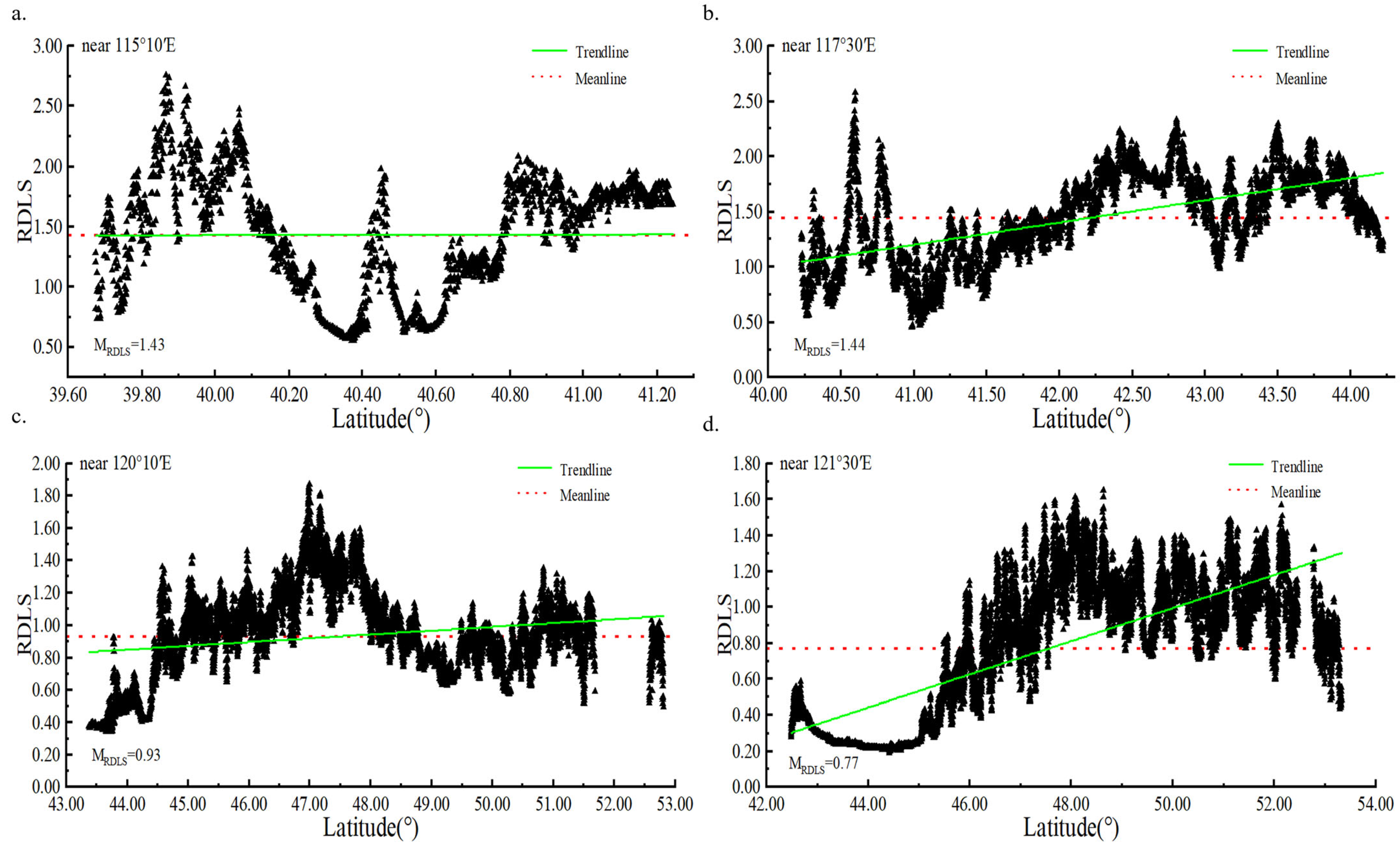
3.2.1. Distribution Characteristics of the RDLS in the Latitude Direction under the Optimal Analysis Window

Under the optimal analysis window, the maximum value of RDLS at and near 41°10′ N occurred at the border of Fengning County and Chicheng County near 116.25° E and was approximately 2.59; the minimum value of RDLS occurred at and near 118° E and was about 0.44, with a mean of approximately 1.27 (Figure 8a). Moreover, 43°45′ N and its vicinity had the maximum value of RDLS at Hexigten Banner near 117.54° E, with an approximate value of 2.28 and a mean value of 0.63 (Figure 8b). The maximum value of RDLS of approximately 47°4′ N occurred in the Greater Khingan Mountains near 120.52° E, with an approximate value of 2.10 and a mean value of approximately 0.94 (Figure 8c). In all three latitudinal belts, the RDLS showed the same trend: it was greater in the western mountainous areas than in the eastern mountainous plains transition zone (Figure 8a–c). Unlike the other latitudinal belts, the RDLS was greater in the east than in the west and near 49°45′ N (Figure 8d). The maximum value occurred in the Greater Khingan Mountains near 122.40° E at approximately 1.57, with a mean value of approximately 0.89 (Figure 8d), and the minimum value of approximately 0.54 was distributed in the transition zone from the Greater Khingan Mountains to Hulunbuir Grassland in the west (Figure 8d).

In summary, the RDLS in mountainous regions surpassed that in mountain-to-plain transition zone. The lowest latitude of 41°10′ N exhibited the highest overall RDLS, and the four latitudinal zones demonstrated a characteristic decreasing, increasing and decreasing pattern in the RDLS from south to north (Figure 8).

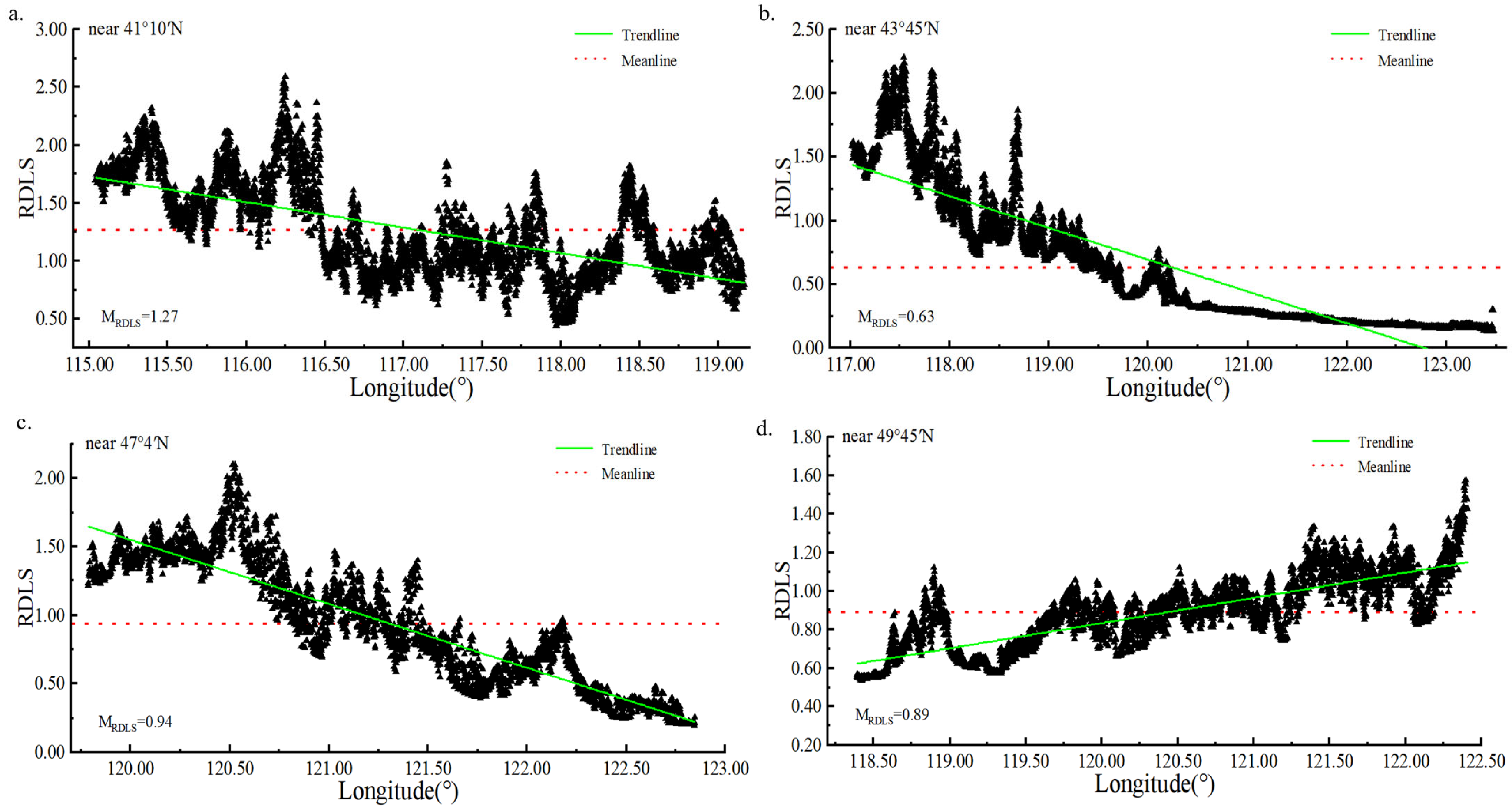
3.2.2. Distribution Characteristics of RDLS in the Longitudinal Direction under Optimal Analysis Window

Under the optimal analysis window, the RDLS in and near 115°10′ E showed a “W”—shaped trend, that is, it increased and decreased with the interphase distribution of mountains and canyons (Figure 9a), and the maximum value at approximately 39.87° N was about 2.76. The lowest value occurred near 40.37° N, and was approximately 0.56, and the mean value was approximately 1.43 (Figure 9a). In the region passing through 117°30′ E, the RDLS in the north was greater than that in the south, but the maximum value appeared near 40.61° N (Figure 9b), at approximately 2.58; the minimum RDLS appeared near 40.99° N, about 0.46, and the mean value was approximately 1.44 (Figure 9b). In the area passing through 120°10′ E, as a whole, the RDLS gradually increased from south to north, reaching a maximum value near 46.70° N, and then gradually decreased to 49.29° N in the north and then slowly increased (Figure 9c). The maximum value was approximately 1.87; the minimum value occurred around 43.74° N and was about 0.34, and the mean RDLS was approximately 0.93 (Figure 9c). Similarly, in the region traversed by 121°30′ E, the RDLS of the northern Greater Khingan Mountains was greater than that of the transition region from the southern mountains to the plain (Figure 9d). The maximum value appeared near 48.64° N, which was approximately 1.65; the minimum value was near 44.42° N and was about 0.19, and the mean RDLS was 0.77 (Figure 9d).

In general, these results were consistent with the latitudinal characteristics. In the longitudinal direction, the RDLS in the mountainous terrain surpassed that in mountain-to-plain transition zone. Overall, the RDLS of the four longitudinal zones tended to be higher in the west and lower in the east (Figure 9).

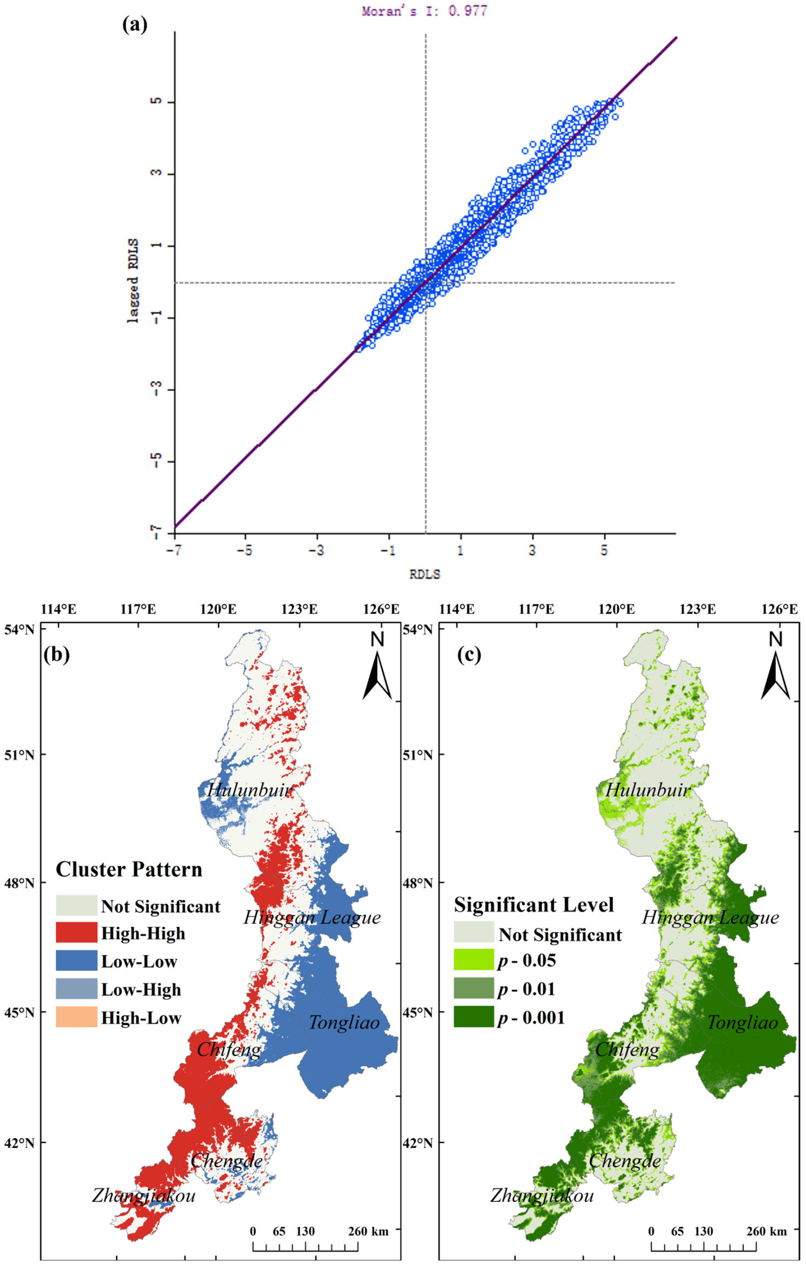
3.3. Spatial Auto-Correlation Analysis and Significance Test

To deepen the comprehensive understanding of the spatial distribution of RDLS in the study area better, the 1 km × 1 km grid was employed to resample the data, and 341,854 sample points were collected from RDLS raster image. Spatial dependence can be characterized by assessing whether a variable exhibits spatial correlation and determining the extent of that correlation. In this study, we employed a conditional permutation method with 999 conditional permutations to test the statistical significance of the global Moran’s I. A high z-score and a low pseudo p-value strongly demonstrated that the calculated global Moran’s I was statistically significant [61]. The results indicated a statistically significant global Moran’s I statistic (Moran’s I equal to 0.977, z-value equal to 1082.32 and p-value equal to 0.001). The results imply that the RDLS was not due to completely spatial random processes (Figure 10a). The scatter points are primarily concentrated in first and third quadrants (Figure 10a), indicating that the RDLS had a spatial positive correlation.

The LISA cluster map is capable of intuitively reflects the spatial distribution of “HH”, “LL”, “HL” and “LH”. And the LISA significance map can embody the spatial significance level of the RDLS [53]. The local spatial correlation pattern of the RDLS was analyzed using the LISA clustering map and LISA significance level map (Figure 10b,c). The significant level of 0.001 was primarily concentrated in “HH” and “LL” in which RDLS had a strong correlation. The “HH” region was located on the mountain, and “LL” was in the transition zone from mountain to plain. The regions with significance levels of 0.01 and 0.05 were primarily located on the vicinity of the zones for which the significance level reached 0.001 (Figure 10b,c).

3.4. Correlation Analysis among RDLS and Both Mean Elevation and Relative Elevation Difference

Statistical analysis of the RDLS with mean elevation and relative elevation difference in northern China’s forest-steppe ecotone was performed at the raster level. The results show that, under the optimal analysis window, RDLS was linearly positively correlated with the mean elevation and relative elevation difference; that is, the RDLS increased linearly with the increased of the mean elevation and relative elevation difference (Figure 11). The linear fitting relationship between mean elevation and RDLS was represented as y = 801.57x + 31.01 (R² = 0.951), and the linear fitting relationship between relative elevation difference and RDLS was represented as y = 137.66x − 21.51 (R² = 0.544) (Figure 11).

4. Discussion

(1) Topographical factors have a significant effect on the local climate, geologic hazards, the path and speed of fire spreading, the migrations of wild animals, and the runoff path and speed of precipitation. Topographic relief is a quantitative indicator to describe the surface morphology [7], which has been widely used in many fields [1,2,6,8,13,15]. However, most of the existing studies have regarded topographic relief as the difference between the highest and lowest points in a given area [5,40]. This method is easy to understand, but the calculation is too simple. In this study, the RDLS model [50] was adopted, and it was regarded as the relief situation represented by the proportion of elevation change and flat land in a certain region [50]. Based on the extraction of relative elevation difference, the method considers the impact of elevation, relative elevation difference, and flat and non-flat area on the topographic relief; thus, it is more scientific and rigorous.

(2) The key to extracting topographic relief is to determine the optimal statistical unit. The traditional calculation method has the disadvantages of the high impact of subjectivity, a tendency to multiple inflection points, and large uncertainty in the test method [64]. The mean change-point analysis method is effective for the test of unique inflection points and is an ideal method for determining the optimal statistical unit [1,38]. In the study, the mean change-point method was employed to identify the optimal window of the RDLS of northern China’s forest-steppe ecotone. The results showed that the optimal window was 29 × 29 (rectangular neighborhood), covering approximately 0.76 km².

(3) Under the optimal window, the RDLS in study area ranged from 0.084 to 3.516, with a mean of 0.887. Notably, 98.52% of the RDLS in the region was concentrated in the 0.084–1.934 range, with peaks at 0.198 and 0.962. The topographic relief in our study was significantly lower than that in a similar region, northeast China [64], because the study in northeast China only used the pixel elevation difference as the topographic relief, while the RDLS model adopted in our study (Formula 4) considered the relative elevation difference, as well as the relationship among mean elevation, relative elevation difference, and non-flat area to extract topographic relief. These two methods are different. Our results are consistent with those of existing research using the same research method [38].

(4) In terms of latitudinal and longitudinal distribution, the RDLS of latitudinal zones exhibited a decreasing, increasing, then decreasing trend from south to north, with the lowest latitude of 41°10′ N having the highest overall RDLS. The RDLS of longitudinal zones displayed a high-west to low-east characteristic. Overall, in northern China’s forest-steppe ecotone, the RDLS of mountainous terrain was greater than that in mountain-to-plain transition zone.

(5) Under optimal analysis window, the RDLS increased linearly with the increase of the mean elevation and relative elevation difference. This result is consistent with the existing research, which studied on the RDLS of the Tibetan Plateau [49]. However, the RDLS of the Tibet Plateau had obvious stage changes with the mean elevation and relative elevation change [49], whereas the RDLS in our study area was always linearly positively correlated with mean elevation and relative elevation difference. This difference is due to the topography of the Tibetan Plateau, which is distributed in a stepped pattern, and there are many areas with significant relative height differences at the edge of the plateau (e.g., the transition zone from the Sichuan Basin to the Tibetan Plateau, the western Sichuan region, the Yarlung Zangbu Grand Canyon, and the Hengduan Mountain area in southern Tibetan Plateau). The interior of the plateau has relatively flat areas but also a large distribution of mountain ranges (e.g., Bayankala Mountain and Tanggula Mountain). In our study area, the elevation is lower, and the mountain topography varies more gently than in the Tibetan Plateau.

(6) In the future, the following points should be considered in the process of ecological planning, implementation of ecological projects, and ecological management in the study area and similar regions: (1) The topographic relief has a significant effect on the local climate; for example, the temperature, humidity, and light conditions differ between sunny and shady slopes. These differences affect plant growth. Thus, the study area should give full consideration to the topographic conditions when implementing afforestation projects and select suitable tree or grass species to promote ecological recovery. (2) Complex terrain may cause species isolation. When planning ecological corridors in the study area, considering topographic relief to ensure the connectivity of the corridors and promoting wildlife migration and biodiversity protection is necessary. (3) Topography relief affects the runoff path and speed of precipitation, affecting soil thickness and fertility. Soil conservation measures should be strengthened in areas with large fluctuations to prevent soil and water erosion. (4) Geological hazards such as landslides are more likely to occur in areas with high relief. By analyzing topographic relief, potential areas of high geologic hazards can be identified so that appropriate prevention and control measures can be developed. (5) In addition, topography also affects the path and speed of fire spreading. Thus, the planning and construction of fire prevention roads and fire isolation belts in the study area need to consider the topographic relief to improve fire prevention efficiency.

5. Conclusions

In this study, the RDLS of the forest-steppe ecotone in northern China was studied using elevation data based on the window analysis method, mean change-point method, the RDLS model, and spatial autocorrelation method. The results showed that the mean change-point method can effectively identify the optimal window for the analysis of the RDLS of the region. The RDLS in the forest-steppe intertwined zone in northern China had significant spatial clustering, with the high-value areas mainly located in mountainous areas and the low-value areas in mountain-to-plain transition zone; the RDLS between different administrative units and different watersheds all had obvious variability. Topographic relief has a significant effect on the local climate, geologic hazards, the path and speed of fire spreading, the migrations of wild animals, and the runoff path and speed of precipitation. Therefore, in the future, the implementation of ecological projects in this area should take into full consideration the topographical conditions and scientifically implement the afforestation planning, aim to improve the ecological benefits of the ecological projects. The results of the study are practical and policy-relevant, and they can provide a reference for ecological planning in this region and similar areas, further promoting the construction of the national ecological security barrier. Due to space limitations, the existing vegetation structure was not analyzed in this study. In the future, forestry data can be combined to analyze the existing stand structure in the study area and explore the relationship between site conditions and stand structure, providing references for forest management.

References

1. Wang, B.; Cheng, W. Effects of Land Use/Cover on Regional Habitat Quality under Different Geomorphic Types Based on InVEST Model. Remote Sens. 2022, 14, 1279. [Google Scholar] [CrossRef]
2. Liu, Y.; Chen, J.; Sun, X.; Li, Y.; Zhang, Y.; Xu, W.; Yan, J.; Ji, Y.; Wang, Q. A Progressive Framework Combining Unsupervised and Optimized Supervised Learning for Debris Flow Susceptibility Assessment. CATENA 2024, 234, 107560. [Google Scholar] [CrossRef]
3. Wang, Z.; Hu, Z.; Liu, H.; Gong, H.; Zhao, W.; Yu, M.; Zhang, M. Application of the Relief Degree of Land Surface in Landslide Disasters Susceptibility Assessment in China. In Proceedings of the 2010 18th International Conference on Geoinformatics, Beijing, China, 18–20 June 2010; pp. 1–5. [Google Scholar]
4. Wu, J.; Zhang, Y.; Yang, L.; Zhang, Y.; Lei, J.; Zhi, M.; Ma, G. Identifying the Essential Influencing Factors of Landslide Susceptibility Models Based on Hybrid-Optimized Machine Learning with Different Grid Resolutions: A Case of Sino-Pakistani Karakorum Highway. Environ. Sci. Pollut. Res. 2023, 30, 100675–100700. [Google Scholar] [CrossRef]
5. Yang, Z.; Pang, B.; Dong, W.; Li, D.; Huang, Z. Interaction of Landslide Spatial Patterns and River Canyon Landforms: Insights into the Three Parallel Rivers Area, Southeastern Tibetan Plateau. Sci. Total Environ. 2024, 914, 169935. [Google Scholar] [CrossRef]
6. Yang, N.; Jiang, L.; Chao, Y.; Li, Y.; Liu, P. Influence of Relief Degree of Land Surface on Street Network Complexity in China. ISPRS Int. J. Geo-Inf. 2021, 10, 705. [Google Scholar] [CrossRef]
7. Sui, G.; Hao, B.; Feng, G.; Sun, B. Data Analysis of Elevation Standard Deviation Classifying Geomorphological Types. In Proceedings of the 2010 International Conference on Computer Application and System Modeling (ICCASM 2010), Taiyuan, China, 22–24 October 2010; pp. V15-294–V15-297. [Google Scholar] [CrossRef]
8. Chen, S.; Wang, X.; Lin, Q. Spatial Pattern Characteristics and Influencing Factors of Mountainous Rural Settlements in Metropolitan Fringe Area: A Case Study of Pingnan County, Fujian Province. Heliyon 2024, 10, e26606. [Google Scholar] [CrossRef]
9. Li, Y.; Du, J.; Ran, D.; Yi, C. Spatio-Temporal Distribution and Evolution of the Tujia Traditional Settlements in China. PLoS ONE 2024, 19, e0299073. [Google Scholar] [CrossRef]
10. Liu, Y.; Deng, W.; Song, X. Relief Degree of Land Surface and Population Distribution of Mountainous Areas in China. J. Mt. Sci. 2015, 12, 518–532. [Google Scholar] [CrossRef]
11. Wu, W.; Niu, S. Evolutional Analysis of Coupling between Population and Resource-Environment in China. Procedia Environ. Sci. 2012, 12, 793–801. [Google Scholar] [CrossRef]
12. Yang, Y.; Feng, Z.; Wang, L.; You, Z. Research on the Suitability of Population Distribution at the Provincial Scale in China. J. Geogr. Sci. 2014, 24, 889–906. [Google Scholar] [CrossRef]
13. Huang, D.; Su, L.; Fan, H.; Zhou, L.; Tian, Y. Identification of Topographic Factors for Gully Erosion Susceptibility and Their Spatial Modelling Using Machine Learning in the Black Soil Region of Northeast China. Ecol. Indic. 2022, 143, 109376. [Google Scholar] [CrossRef]
14. Deng, J.; Cheng, W.; Liu, Q.; Jiao, Y.; Liu, J. Morphological Differentiation Characteristics and Classification Criteria of Lunar Surface Relief Amplitude. J. Geogr. Sci. 2022, 32, 2365–2378. [Google Scholar] [CrossRef]
15. Jiang, W.; Pan, H.; Yang, N.; Xiao, H. Dam Inundation Duration as a Dominant Constraint on Riparian Vegetation Recovery. Sci. Total Environ. 2023, 904, 166427. [Google Scholar] [CrossRef]
16. Jin, H.; Zhong, R.; Liu, M.; Ye, C.; Chen, X. Spatial Risk Occurrence of Extreme Precipitation in China under Historical and Future Scenarios. Nat. Hazards 2023, 119, 2033–2062. [Google Scholar] [CrossRef]
17. Pan, W.; Wang, J.; Li, Y.; Chen, S.; Lu, Z. Spatial Pattern of Urban-Rural Integration in China and the Impact of Geography. Geogr. Sustain. 2023, 4, 404–413. [Google Scholar] [CrossRef]
18. Chen, Y.; Li, Y.; Wang, L.; Duan, Y.; Cao, W.; Wang, X.; Li, Y. Heterogeneity of Leaf Stoichiometry of Different Life Forms along Environmental Transects in Typical Ecologically Fragile Areas of China. Sci. Total Environ. 2024, 910, 168495. [Google Scholar] [CrossRef]
19. Du, X.-F.; Liu, H.-W.; Li, Y.-B.; Li, B.; Han, X.; Li, Y.-H.; Mahamood, M.; Li, Q. Soil Community Richness and Composition Jointly Influence the Multifunctionality of Soil along the Forest-Steppe Ecotone. Ecol. Indic. 2022, 139, 108900. [Google Scholar] [CrossRef]
20. Wang, L.; Jia, Z.; Li, Q.; He, L.; Tian, J.; Ding, W.; Liu, T.; Gao, Y.; Zhang, J.; Han, D.; et al. Grazing Impacts on Soil Enzyme Activities Vary with Vegetation Types in the Forest-Steppe Ecotone of Northeastern China. Forests 2023, 14, 2292. [Google Scholar] [CrossRef]
21. Li, B.; Li, Y.; Fanin, N.; Han, X.; Du, X.; Liu, H.; Li, Y.; Li, Q. Adaptation of Soil Micro-Food Web to Elemental Limitation: Evidence from the Forest-Steppe Ecotone. Soil Biol. Biochem. 2022, 170, 108698. [Google Scholar] [CrossRef]
22. Schmidt, M.; Jochheim, H.; Kersebaum, K.-C.; Lischeid, G.; Nendel, C. Gradients of Microclimate, Carbon and Nitrogen in Transition Zones of Fragmented Landscapes—A Review. Agric. For. Meteorol. 2017, 232, 659–671. [Google Scholar] [CrossRef]
23. Erdős, L.; Ambarlı, D.; Anenkhonov, O.A.; Bátori, Z.; Cserhalmi, D.; Kiss, M.; Kröel-Dulay, G.; Liu, H.; Magnes, M.; Molnár, Z.; et al. The Edge of Two Worlds: A New Review and Synthesis on Eurasian Forest-Steppes. Appl. Veg. Sci. 2018, 21, 345–362. [Google Scholar] [CrossRef]
24. He, P.; Fontana, S.; Ma, C.; Liu, H.; Xu, L.; Wang, R.; Jiang, Y.; Li, M.-H. Using Leaf Traits to Explain Species Co-Existence and Its Consequences for Primary Productivity across a Forest-Steppe Ecotone. Sci. Total Environ. 2023, 859, 160139. [Google Scholar] [CrossRef]
25. Liu, F.; Liu, H.; Xu, C.; Zhu, X.; He, W.; Qi, Y. Remotely Sensed Birch Forest Resilience against Climate Change in the Northern China Forest-Steppe Ecotone. Ecol. Indic. 2021, 125, 107526. [Google Scholar] [CrossRef]
26. Hou, G.; Delang, C.O.; Lu, X. Afforestation Changes Soil Organic Carbon Stocks on Sloping Land: The Role of Previous Land Cover and Tree Type. Ecol. Eng. 2020, 152, 105860. [Google Scholar] [CrossRef]
27. Zhang, Z.; Hao, M.; Li, Y.; Shao, Z.; Yu, Q.; He, Y.; Gao, P.; Xu, J.; Dun, X. Effects of Vegetation and Terrain Changes on Spatial Heterogeneity of Soil C–N–P in the Coastal Zone Protected Forests at Northern China. J. Environ. Manag. 2022, 317, 115472. [Google Scholar] [CrossRef]
28. Zethof, J.H.T.; Cammeraat, E.L.H.; Nadal-Romero, E. The Enhancing Effect of Afforestation over Secondary Succession on Soil Quality under Semiarid Climate Conditions. Sci. Total Environ. 2019, 652, 1090–1101. [Google Scholar] [CrossRef]
29. Jandl, R.; Lindner, M.; Vesterdal, L.; Bauwens, B.; Baritz, R.; Hagedorn, F.; Johnson, D.W.; Minkkinen, K.; Byrne, K.A. How Strongly Can Forest Management Influence Soil Carbon Sequestration? Geoderma 2007, 137, 253–268. [Google Scholar] [CrossRef]
30. Tang, X.; Zhao, X.; Bai, Y.; Tang, Z.; Wang, W.; Zhao, Y.; Wan, H.; Xie, Z.; Shi, X.; Wu, B.; et al. Carbon Pools in China’s Terrestrial Ecosystems: New Estimates Based on an Intensive Field Survey. Proc. Natl. Acad. Sci. USA 2018, 115, 4021–4026. [Google Scholar] [CrossRef]
31. Zhang, Y.; Zhao, X.; Gong, J.; Luo, F.; Pan, Y. Effectiveness and Driving Mechanism of Ecological Restoration Efforts in China from 2009 to 2019. Sci. Total Environ. 2024, 910, 168676. [Google Scholar] [CrossRef]
32. He, J.; Shi, X. Detection of Social-Ecological Drivers and Impact Thresholds of Ecological Degradation and Ecological Restoration in the Last Three Decades. J. Environ. Manag. 2022, 318, 115513. [Google Scholar] [CrossRef]
33. Liu, Y.; Gao, P.; Zhang, L.; Niu, X.; Wang, B. Spatial Heterogeneity Distribution of Soil Total Nitrogen and Total Phosphorus in the Yaoxiang Watershed in a Hilly Area of Northern China Based on Geographic Information System and Geostatistics. Ecol. Evol. 2016, 6, 6807–6816. [Google Scholar] [CrossRef]
34. Zhao, C.; Liu, J.; Mou, W.; Zhao, W.; Zhou, Z.; Ta, F.; Lei, L.; Li, C. Topography Shapes the Carbon Allocation Patterns of Alpine Forests. Sci. Total Environ. 2023, 898, 165542. [Google Scholar] [CrossRef]
35. Cheng, Y.; Liu, H.; Wang, H.; Hao, Q. Differentiated Climate-Driven Holocene Biome Migration in Western and Eastern China as Mediated by Topography. Earth-Sci. Rev. 2018, 182, 174–185. [Google Scholar] [CrossRef]
36. Hao, Q.; Liu, H.; Liu, X. Pollen-Detected Altitudinal Migration of Forests during the Holocene in the Mountainous Forest–Steppe Ecotone in Northern China. Palaeogeogr. Palaeoclimatol. Palaeoecol. 2016, 446, 70–77. [Google Scholar] [CrossRef]
37. Yin, Y.; Liu, H.; Liu, G.; Hao, Q.; Wang, H. Vegetation Responses to Mid-Holocene Extreme Drought Events and Subsequent Long-Term Drought on the Southeastern Inner Mongolian Plateau, China. Agric. For. Meteorol. 2013, 178–179, 3–9. [Google Scholar] [CrossRef]
38. Zhang, J.; Zhu, W.; Zhu, L.; Cui, Y.; He, S.; Ren, H. Topographical Relief Characteristics and Its Impact on Population and Economy: A Case Study of the Mountainous Area in Western Henan, China. J. Geogr. Sci. 2019, 29, 598–612. [Google Scholar] [CrossRef]
39. Yang, Z.; Hong, Y.; Guo, Q.; Yu, X.; Zhao, M. The Impact of Topographic Relief on Population and Economy in the Southern Anhui Mountainous Area, China. Sustainability 2022, 14, 14332. [Google Scholar] [CrossRef]
40. Liu, S.; Cui, Y.; Lu, F.; Qin, X. The Analysis of Relief Amplitude in Qinghai Province Based on GIS. In Proceedings of the 2013 21st International Conference on Geoinformatics, Kaifeng, China, 20–22 June 2013; pp. 1–5. [Google Scholar]
41. Cheng, Y.; Liu, H.; Dong, Z.; Duan, K.; Wang, H.; Han, Y. East Asian Summer Monsoon and Topography Co-Determine the Holocene Migration of Forest-Steppe Ecotone in Northern China. Glob. Planet. Chang. 2020, 187, 103135. [Google Scholar] [CrossRef]
42. Li, Y.; Qin, Y. The Response of Net Primary Production to Climate Change: A Case Study in the 400 mm Annual Precipitation Fluctuation Zone in China. Int. J. Environ. Res. Public Health 2019, 16, 1497. [Google Scholar] [CrossRef]
43. Li, Y.; Xie, Z.; Qin, Y.; Zheng, Z. Estimating Relations of Vegetation, Climate Change, and Human Activity: A Case Study in the 400 mm Annual Precipitation Fluctuation Zone, China. Remote Sens. 2019, 11, 1159. [Google Scholar] [CrossRef]
44. Zhang, X.; Liu, L.; Chen, X.; Gao, Y.; Xie, S.; Mi, J. GLC_FCS30: Global Land-Cover Product with Fine Classification System at 30 m Using Time-Series Landsat Imagery. Earth Syst. Sci. Data 2021, 13, 2753–2776. [Google Scholar] [CrossRef]
45. Zhang, X.; Liu, L.; Zhao, T.; Gao, Y.; Chen, X.; Mi, J. GISD30: Global 30 m Impervious-Surface Dynamic Dataset from 1985 to 2020 Using Time-Series Landsat Imagery on the Google Earth Engine Platform. Earth Syst. Sci. Data 2022, 14, 1831–1856. [Google Scholar] [CrossRef]
46. Zhang, X.; Liu, L.; Zhao, T.; Chen, X.; Lin, S.; Wang, J.; Mi, J.; Liu, W. GWL_FCS30: A Global 30 m Wetland Map with a Fine Classification System Using Multi-Sourced and Time-Series Remote Sensing Imagery in 2020. Earth Syst. Sci. Data 2023, 15, 265–293. [Google Scholar] [CrossRef]
47. Grohmann, C.H. Evaluation of TanDEM-X DEMs on Selected Brazilian Sites: Comparison with SRTM, ASTER GDEM and ALOS AW3D30. Remote Sens. Environ. 2018, 212, 121–133. [Google Scholar] [CrossRef]
48. Del Rosario González-Moradas, M.; Viveen, W.; Andrés Vidal-Villalobos, R.; Carlos Villegas-Lanza, J. A Performance Comparison of SRTM v. 3.0, AW3D30, ASTER GDEM3, Copernicus and TanDEM-X for Tectonogeomorphic Analysis in the South American Andes. CATENA 2023, 228, 107160. [Google Scholar] [CrossRef]
49. Feng, Z.; Li, W.; Li, P.; Xiao, C. Relief degree of land surface and its geographical meanings in the Qinghai-Tibet Plateau, China. Acta Geogr. Sin. 2020, 75, 1359–1372. [Google Scholar] [CrossRef]
50. Feng, Z.; Tang, Y.; Yang, Y.; Zhang, D. Relief Degree of Land Surface and Its Influence on Population Distribution in China. J. Geogr. Sci. 2008, 18, 237–246. [Google Scholar] [CrossRef]
51. Zhang, L.; Fang, C.; Zhao, R.; Zhu, C.; Guan, J. Spatial–Temporal Evolution and Driving Force Analysis of Eco-Quality in Urban Agglomerations in China. Sci. Total Environ. 2023, 866, 161465. [Google Scholar] [CrossRef]
52. Deng, Y.; Ling, Z.; Jiang, W. Urban Water Bodies in China: Spatial Distribution Patterns, Temporal Change Characteristics, and Relationship with Economic Development. Ecol. Indic. 2023, 157, 111139. [Google Scholar] [CrossRef]
53. Jing, Y.; Zhang, F.; He, Y.; Kung, H.; Johnson, V.C.; Arikena, M. Assessment of Spatial and Temporal Variation of Ecological Environment Quality in Ebinur Lake Wetland National Nature Reserve, Xinjiang, China. Ecol. Indic. 2020, 110, 105874. [Google Scholar] [CrossRef]
54. Anselin, L.; Li, X. Operational Local Join Count Statistics for Cluster Detection. J. Geogr. Syst. 2019, 21, 189–210. [Google Scholar] [CrossRef] [PubMed]
55. Kabos, S.; Csillag, F. The Analysis of Spatial Association on a Regular Lattice by Join-Count Statistics without the Assumption of First-Order Homogeneity. Comput. Geosci. 2002, 28, 901–910. [Google Scholar] [CrossRef]
56. Shakiba, M.; Lake, L.W.; Gale, J.F.W.; Pyrcz, M.J. Multiscale Spatial Analysis of Fracture Arrangement and Pattern Reconstruction Using Ripley’s K-Function. J. Struct. Geol. 2022, 155, 104531. [Google Scholar] [CrossRef]
57. Liu, J.; Kang, H.; Tao, W.; Li, H.; He, D.; Ma, L.; Tang, H.; Wu, S.; Yang, K.; Li, X. A Spatial Distribution—Principal Component Analysis (SD-PCA) Model to Assess Pollution of Heavy Metals in Soil. Sci. Total Environ. 2023, 859, 160112. [Google Scholar] [CrossRef] [PubMed]
58. Awaleh, M.O.; Boschetti, T.; Ahmed, M.M.; Dabar, O.A.; Robleh, M.A.; Waberi, M.M.; Ibrahim, N.H.; Dirieh, E.S. Spatial Distribution, Geochemical Processes of High-Content Fluoride and Nitrate Groundwater, and an Associated Probabilistic Human Health Risk Appraisal in the Republic of Djibouti. Sci. Total Environ. 2024, 927, 171968. [Google Scholar] [CrossRef] [PubMed]
59. He, S.; Yang, H.; Chen, X.; Wang, D.; Lin, Y.; Pei, Z.; Li, Y.; Akbar Jamali, A. Ecosystem Sensitivity and Landscape Vulnerability of Debris Flow Waste-Shoal Land under Development and Utilization Changes. Ecol. Indic. 2024, 158, 111335. [Google Scholar] [CrossRef]
60. Zhang, C.; Zhao, L.; Zhang, H.; Chen, M.; Fang, R.; Yao, Y.; Zhang, Q.; Wang, Q. Spatial-Temporal Characteristics of Carbon Emissions from Land Use Change in Yellow River Delta Region, China. Ecol. Indic. 2022, 136, 108623. [Google Scholar] [CrossRef]
61. Anselin, L. Local Indicators of Spatial Association—LISA. Geogr. Anal. 1995, 27, 93–115. [Google Scholar] [CrossRef]
62. Gedamu, W.T.; Plank-Wiedenbeck, U.; Wodajo, B.T. A Spatial Autocorrelation Analysis of Road Traffic Crash by Severity Using Moran’s I Spatial Statistics: A Comparative Study of Addis Ababa and Berlin Cities. Accid. Anal. Prev. 2024, 200, 107535. [Google Scholar] [CrossRef] [PubMed]
63. Ijumulana, J.; Ligate, F.; Bhattacharya, P.; Mtalo, F.; Zhang, C. Spatial Analysis and GIS Mapping of Regional Hotspots and Potential Health Risk of Fluoride Concentrations in Groundwater of Northern Tanzania. Sci. Total Environ. 2020, 735, 139584. [Google Scholar] [CrossRef] [PubMed]
64. Wang, R.H.; Zhang, S.W.; Pu, L.; Li, F.; Wang, Q.; Chen, D.; Yang, J.; Chang, L.; Bu, K. Analysis on the relief amplitude in northeast China based on ASTER GDEM and mean change point method. J. Arid. Land Resour. Environ. 2016, 30, 49–54. [Google Scholar] [CrossRef]
Figure 1. Location map of study area: (a) map of China; (b) boundaries of study area; (c) vegetation field survey map; (d) digital elevation model map.
Forests 15 01122 g001
Figure 2. Spatial distribution of RDLS under random window size: (a) 16 × 16; (b) 35 × 35; (c) 56 × 56; (d) 78 × 78.
Forests 15 01122 g002
Figure 3. Changes in land area proportion corresponding to RDLS under random window size.
Forests 15 01122 g003
Figure 4. (a) Relationship between relative elevation difference and window areas; (b) proportion curves of SSk.
Forests 15 01122 g004
Figure 5. Spatial distribution of RDLS of different grades under optimal analysis window.
Forests 15 01122 g005
Figure 6. Land area proportion curve corresponding to RDLS of different grades.
Forests 15 01122 g006
Figure 7. Mean of RDLS of each city (a), county (b), and basin (c) under optimal analysis window.
Forests 15 01122 g007
Figure 8. Latitudinal distribution features of the RDLS: (a) near 41°10′ N; (b) near 43°45′ N; (c) near 47°4′ N; (d) near 49°45′ N.
Forests 15 01122 g008
Figure 9. Longitudinal distribution features of the RDLS: (a) near 115°10′ E; (b) near 117°30′ E; (c) near 120°10′ E; (d) near 121°30′ E.
Forests 15 01122 g009
Figure 10. Global Moran’s I (a), local Moran’s I (b), and the significance level (c) of RDLS.
Forests 15 01122 g010
Figure 11. Correlation analysis among RDLS and both average elevation and relative elevation difference.
Forests 15 01122 g011
Disclaimer/Publisher’s Note: The statements, opinions and data contained in all publications are solely those of the individual author(s) and contributor(s) and not of MDPI and/or the editor(s). MDPI and/or the editor(s) disclaim responsibility for any injury to people or property resulting from any ideas, methods, instructions or products referred to in the content.