Analysis of Long-Term Vegetation Trends and Their Climatic Driving Factors in Equatorial Africa

Abstract

Understanding vegetation seasonality and its driving mechanisms improves decision-making in the management of ecological systems in a warming global climate. Using multiple statistical methods (i.e., trend analysis, abrupt changes, and partial correlation analysis), this study analyzed the spatiotemporal variations in the Normalized Difference Vegetation Index (NDVI) in the Equatorial Africa (EQA) region and their responses to climate factors from 1982 to 2021. The NDVI values declined at a rate of 0.00023 year⁻¹, while the precipitation (P) and mean temperature (TMEAN) values increased at rates of 0.22 mm year⁻¹ and 0.22 °C year⁻¹, respectively. The mean minimum temperature (TMIN) had a higher rate of 0.2 °C year⁻¹ than the mean maximum temperature (TMAX) at 0.02 °C year⁻¹. An abrupt change analysis showed that the TMAX, P, and NDVI breakpoints occurred in 2000, 2002, and 2009, respectively; TMEAN and TMIN breakpoints occurred in 2001. The NDVI trends declined in forest and cropland areas but increased in shrubland and grassland areas. The summer NDVI trends declined for all vegetation types and were reversed in the winter season. The NDVI positively correlated with the P (r = 0.50) and TMEAN (r = 0.60). All seasonal analyses varied across four seasons. A temporal analysis was conducted using partial correlation analysis (PCR), and the results revealed that TMIN had a greater impact on the NDVI (PCR = −0.45), followed by the TMAX (PCR = 0.31) and then the P (PCR = −0.19). The annual trend showed that areas with significant greening were consistent with stronger wetter and weaker warming trends. Both precipitation and temperature showed a positive relationship with vegetation in semi-arid and arid regions but a negative relationship with humid regions. Our findings improve our insight into scientific knowledge on ecological conservation.

1. Introduction

Terrestrial vegetation is a dominant component of terrestrial ecosystems on Earth. Vegetation is an intermediary in the biosphere that influences energy–water–carbon cycles [1,2]. Therefore, monitoring and tracking vegetation dynamics are essential practices in the management of multiple sectors of ecological systems in a warming global climate [3,4]. Recent observation and climate modeling studies have indicated that global warming significantly influences climate patterns and vegetation dynamics [5,6]. For example, changes in the hydrological cycle affect soil moisture and vegetation growth. Vegetation, in turn, impacts the climate by altering energy and biogeochemical cycles [7,8]. According to the sixth assessment report of the Intergovernmental Panel on Climate Change (IPCC AR6), global warming is impacting our ecosystems, and these changes are mainly due to natural and anthropogenic causes [7]. The impacts on ecosystems in a given region affect communities whose livelihoods are directly tied to local ecosystems. However, the factors that explain global ecosystem changes vary across space and time [9]. For example, it is well known that intense social pressures on certain global land areas can suppress or promote major ecosystem richness [4]. Typical empirical evidence includes land degradation in the Amazon and Congo rainforests [10,11] and restoration programs (e.g., in China and India [12,13] and greening in the Sahel region [14,15]). Thus, the study of vegetation dynamics (i.e., patterns, seasonality, and relationships) has gained substantial attention in climate change studies [3,4].

With advances in observational remote sensing, it has become more convenient to disentangle the issue of climate impacts on greening. Remote sensing (RS) data offer scalable multi-temporal and multi-spatial analysis solutions. Many RS products are being developed to measure vegetation health, plant phenology, productivity, etc. [16,17,18]. The NDVI (Normalized Difference Vegetation Index) is a commonly used index based on the ratio of red (R) to near-infrared (NIR) reflectance (i.e., NDVI = (NIR − R)/(NIR + R)) [19]. The NDVI is primarily used to determine the health and density of vegetation. This indicator measures vegetated and non-vegetated terrain within the range of +1 and −1, where high NDVI values (near +1) indicate dense green vegetation and low values indicate moisture-stressed vegetation [20]. Multiple NDVI datasets are available for global and regional studies [17]. The Global Inventory Modeling and Mapping Studies of the National Oceanic and Atmospheric Administration/Advanced Very High-Resolution Radiometer Normalized Difference Vegetation Index third generation (GIMMS NOAA/AVHRR NDVI3g) dataset has been widely used to study vegetation greening since the 1980s. Over the past three decades, the GIMMS NOAA/AVHRR NDVI3g dataset has significantly improved our understanding of intra- and inter-annual variations in vegetation activity from regional to global scales [21,22]. Most of these studies have reported large patterns and trends in the magnitude and timing of vegetation activity in the Northern Hemisphere (NH) [23,24,25]. Additionally, increasing (“greening”) or decreasing (“browning”) vegetation trends have been documented over multiple timescales [26]. The trajectories of these vegetation trends have been reported to be gradual or abrupt for global and regional studies [27]. Vegetation greenness in relation to trends in climate has been investigated at different spatial (i.e., global, regional, and watershed) and temporal scales [28].

Climate drivers, such as precipitation and temperature, generally influence vegetation growth. Precipitation and temperature are the two most widely used climate variables in different regions [29]. Despite these numerous studies, the relationship between precipitation or temperature and vegetation dynamics across different climate zones at different timescales is still complex [29,30]. Most of these studies used statistical models to analyze the effect of water and heat conditions on vegetation. Recently, parametric methods have been reported to be unreliable; however, non-parametric methods such as Sen Slope and Mann–Kendall tests are widely used due to their reliability. These methods can be used to determine changes in vegetation dynamics. Some studies used partial correlation and cross-correlational analysis to quantify vegetation-driving factors. The partial correlation analysis is intended to explain the relationships between vegetation growth and the driving factors [31]. In addition, transient disturbances in the time series could be determined during changes in vegetation [29], and the Pettitt test is preferred to detect breakpoints or abrupt changes in vegetation and climate time series in many different regions [29,30].

The Equatorial Africa (EQA) region is located in the tropics, which are geographical zones that regulate hydrological and carbon cycles [32]. Previous studies on vegetation dynamics have been conducted in the Horn of Africa [33] and sub-Saharan Africa [34,35,36,37]. Moreover, recent studies have observed frequent changes in land use and land cover (LULC) across sub-Saharan Africa. Thus, the effects of vegetation dynamics caused by climatic and non-climatic factors make this tropical region a hot spot for land–atmosphere interactions [32,38,39] and, by extension, a test bed for investigation [40]. Moreover, warming at night has been reported to be faster than that during the day in certain global lands (e.g., West Africa and Europe) [41]. However, our insight into vegetation responses to the influences of climate and LUCL remains unclear due to confounding factors, such as trends in minimum and maximum temperatures and land use changes. Therefore, it is essential to strengthen research to understand vegetation dynamics in a warming global climate. This study used the GIMMS NOAA/AVHRR NDVI dataset and precipitation and air surface temperatures (minimum and maximum) from the CRU (Climate Research Units) and AVHRR global LULC datasets, respectively. The objectives of this study are as follows:

(1)

To investigate the spatiotemporal trends in vegetation and climate variables;

(2)

To analyze the main climatic drivers of vegetation variability in the EQA region. All the analyses were conducted in the EQA region from 1982 to 2021.

To the best of our knowledge, further studies on the inter-relationship of vegetation and climate in the region have been recommended to include the effect of minimum and maximum temperatures on vegetation dynamics based on the updated NDVI.

2. Materials and Methods

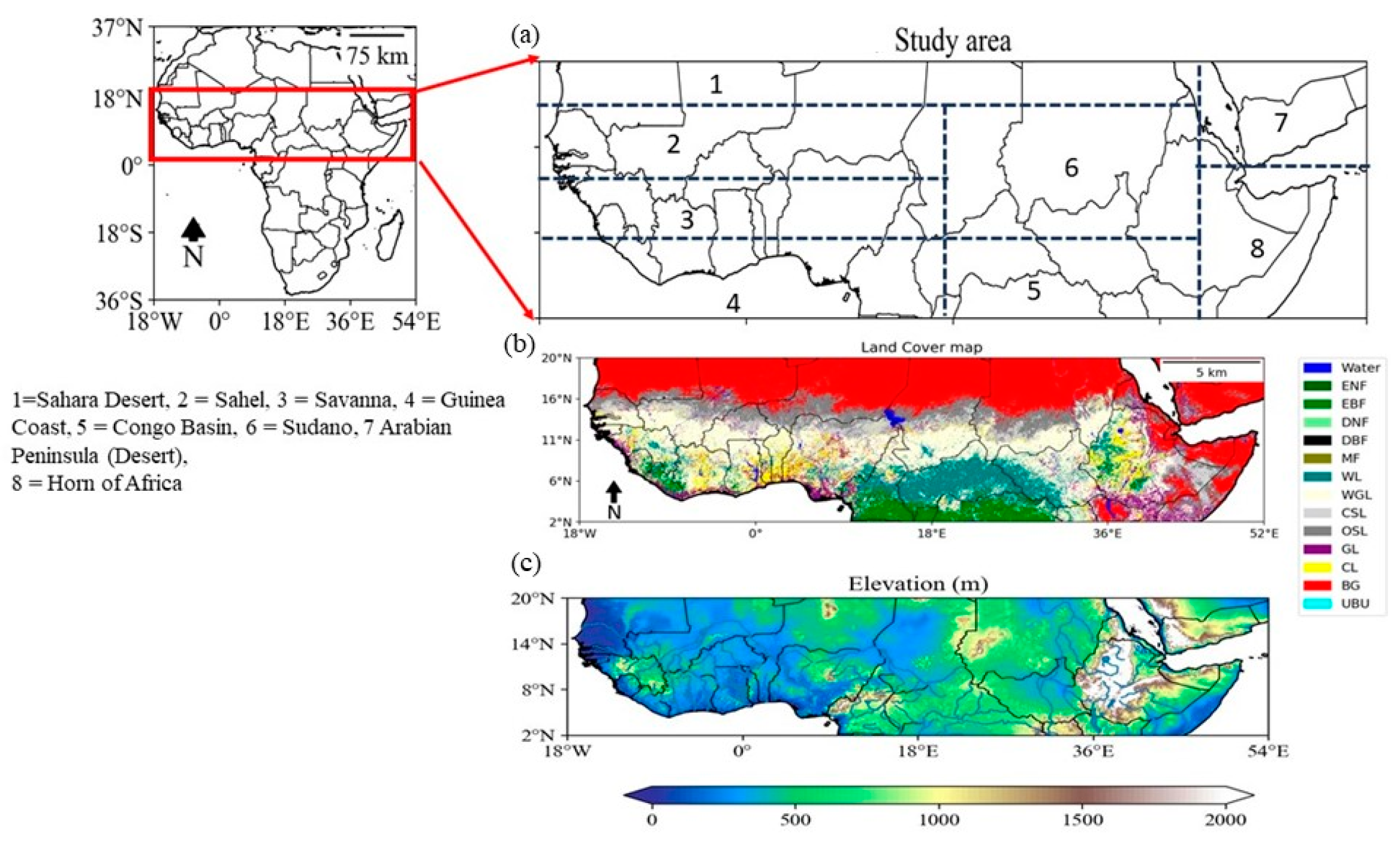
2.1. Study Area

The study area is Equatorial Africa (EQA), which is a region in the tropical African continent with a geographical location of 18° W–55° E longitude and 2° N–20° N latitude. The tropical monsoon climate strongly influences EQA [22,42]. The West African monsoon [22] on the western side and the East African monsoon [42] on the eastern side are prevalent in the region. The average annual precipitation (P) is about 62.76 mm and varies depending on the seasons (summer = 115.48 mm, autumn = 73.01 mm, winter = 9.12 mm, and spring = 53.35 mm). The annual average temperature (TMEAN) is about 26.75 °C and varies depending on the seasons (summer = 27.75 °C, autumn = 26.59 °C, winter = 24.12 °C, and spring = 28.55 °C). The EQA climate system has a distinct wet and dry season [43]. The seasonal climatology values that were computed by the authors, based on the CRU dataset for the period 1982–2021 [44] and averaged over longitude 18° W–55° E and latitude 2° N–20° N, showed that the wettest season was summer and the driest season was winter; the warmest season was spring, and the coolest season was winter. The elevation ranges from 500 to 2000 m above mean sea level [45]. The highest elevations are found in the Ethiopian, Kenyan, and Cameroon highlands (Figure 1c). The ten (10) predominant land cover classification types [46] found in EQA are presented in Figure 1a.

2.2. Data Sources

2.2.1. NDVI

The data used in this study include the Global Inventory Modeling and Mapping Studies (GIMMS) of the National Oceanic and Atmospheric Administration/Advanced Very High-Resolution Radiometer (AVHRR) Normalized Difference Vegetation Index third generation (NDVI3g) (i.e., GIMMS AVHRR NDVI3g) dataset, which includes precipitation, temperature, digital elevation model (DEM), and a land cover map. The GIMMS AVHRR NDVI3g data with a spatial resolution of 8 km and a temporal interval of 15-day compositing periods were obtained from the NASA website (https://daac.ornl.gov/VEGETATION/guides/Global_Veg_Greeness_GIMMS_3G.html, accessed on 10 May 2023). The National Oceanic and Atmospheric Administration/Advanced Very High-Resolution Radiometer Normalized Difference Vegetation Index third generation plus (AVHRR NDVI3g+) dataset covers January 1981 to December 2022 [18,19]. The AVHRR NDVI3g data acquisition process, which includes using various sensor platforms, advanced algorithms for pre-processing, and quality assurance procedures for atmospheric and radiometric correction, has been described in detail in previous studies [18,47]. The Africa region mask was defined to isolate the NDVI region from a gridded global dataset. To convert the bimonthly NDVI to the monthly NDVI, the maximum-value composite (MVC) method proposed by Holben et al. [48] was used. The NDVI grid values range from +1 to −1 and are computed as the ratio of (NIR − R)/(NIR + R) pixels, where NIR is the near-infrared wavelength and R is the red wavelength [18]. Positive NDVI values close to +1 indicate the presence of dense green foliage, while negative NDVI values near −1 indicate the presence of water bodies [49]. We removed negative and zero NDVI grid values that indicated non-vegetated surfaces and water bodies. The pixel grids were set to a monthly mean NDVI value of <0.1 over 39 years [19,50].

2.2.2. Climate Datasets (Precipitation and Temperature)

The Climatic Research Unit (CRU) data were used in this study to compute spatial variation, trends, and correlation between climate and vegetation. The CRU data consist of monthly spans from 1901 to the present with a resolution of 0.5° × 0.5°. The Climatic Research Unit (CRU) dataset was downloaded from the website (http://www.cru.uea.ac.uk, accessed on 10 May 2023). Gridded product data processing and validation were reported by Harris et al. [44]. In addition, the gridded data have been extensively used as they were obtained from over 4000 weather stations and interpolated based on spatial autocorrelation functions [51,52]. The temperature data comprise the monthly mean minimum temperature (TMIN) and the monthly mean maximum temperature (TMAX). The monthly mean temperature (TMEAN) was computed from the TMIN and TMAX, and the study period covered 1982–2021.

2.2.3. Land Use Land Cover

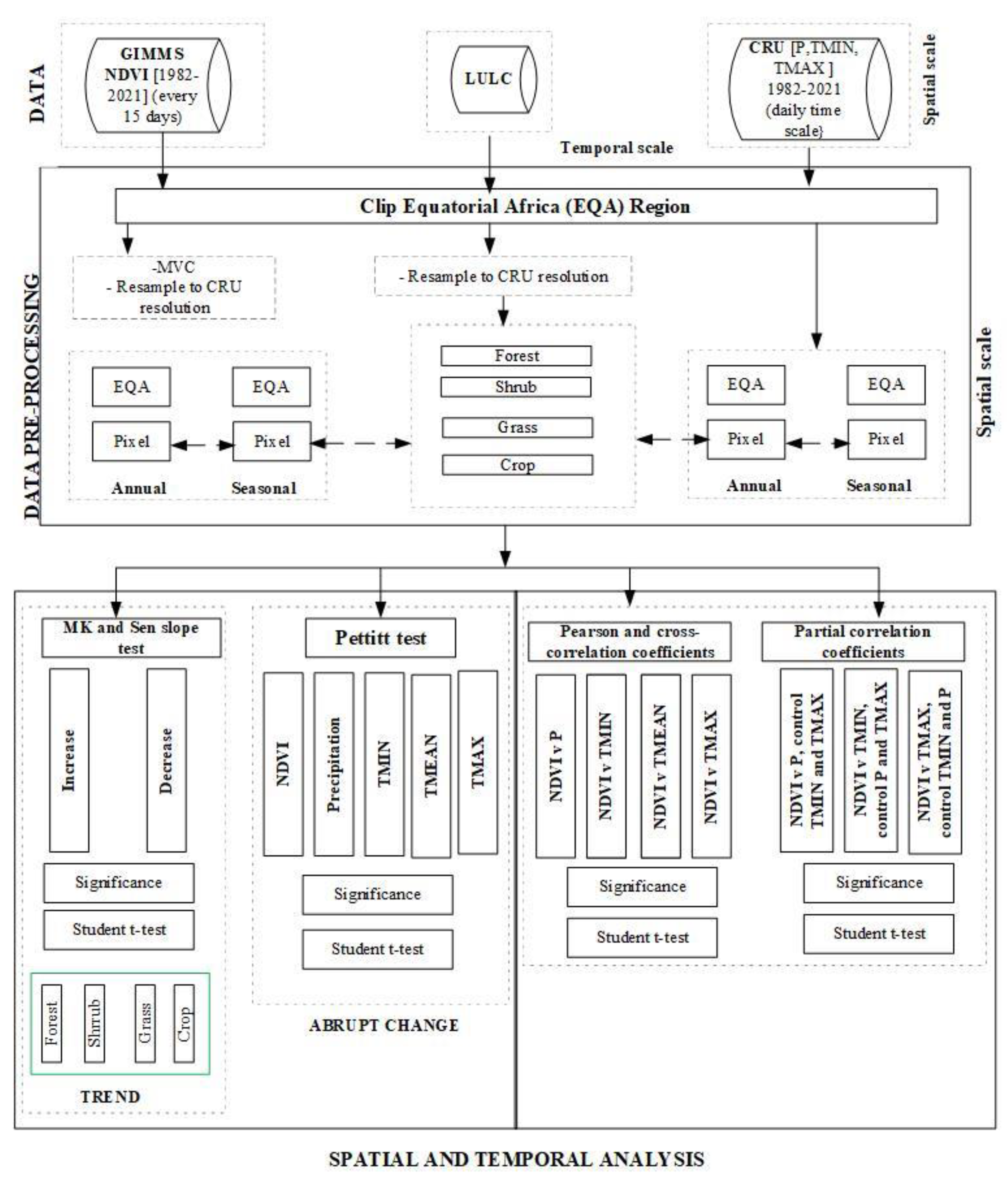
The spatial distribution of land use land cover (LULC) was obtained from the University of Maryland’s Department of Geography through the website https://glad.umd.edu/ (accessed on 10 May 2023) with a spatial resolution of 1 km [46]. Out of the 14 separate land cover types, 10 were regrouped into four predominant land cover classes, including forest, grass, crop, and shrub, which were extracted for further analysis, and non-vegetated cover areas were excluded for consideration in the computation.

2.3. Methods

In this study, we applied various statistical approaches for data analyses.

2.3.1. Data Processing

All data were initially loaded, averaged, and selected from January 1982 to December 2021, and the climatology was calculated by averaging the data from 1982 to 2021 at different time scales. The seasonal scales were defined as a combined monthly average as follows: spring (i.e., March–April–May, MAM), summer (June–July–August, JJA), autumn (September–October–November, SON), and winter (December–January–February, DJF). All datasets were resampled to a spatial resolution of 0.5° × 0.5° using the bilinear interpolation method to match CRU dataset resolution. Figure 2 shows the methodological flow chart of the work.

2.3.2. Statistical Analysis

(a) Trend analysis and significance testcalculation

First, the linear trend was computed to understand the vegetation dynamics and its connections to climate in the EQA region. The linear trend analysis was computed using the non-parametric Mann–Kendall (MK) trend and Sen slope tests. The MK trend test was used to detect the significance of the time series trend, and the Sen slope test was used to compute the magnitude of the trend in the time series [53,54,55,56]. The MK trend test is a non-parametric test on data values (x) of a time series based on Equations (1)–(4) as follows:

$$\mathsf{\upsilon }=\mathrm{f}\left(\mathrm{t}\right)+\sum t$$

(1)

$$\mathrm{S}=\sum _{k-1}^{n-1}\sum _{j=k+1}^{n}sin(x_j-x_k)$$

(2)

where n is the length of the time series $x_i$, … $x_n$, sgn () is the sign function, and $x_j$ and $x_k$ are values in years j and k, respectively. E[S] = 0 for series without a trend and the variance was calculated based on A3 as follows:

$${\delta }^2(\mathrm{S})=\frac{1}{18}\left[n\left(n-1\right)\left(2n+5\right)-\sum _{i=1}^n{t}_n(t_n-1)(2t_n+5)\right]$$

(3)

where n is the number of tied groups and $t_n$ is the number of data values in the nth group. The test statistic Z is as defined in Equation (4):

$$\mathrm{Z}=\left\{\begin{array}{c}\frac{s-1}{\sqrt{{\delta }^2\left(s\right)}}ifS>0\\ 0ifS=0\\ \frac{s+1}{\sqrt{{\delta }^2\left(s\right)}}ifS<0\end{array}\right.$$

(4)

The Z-statistics test the null hypothesis (Ho), which states that there is no trend, against the alternative hypothesis (H1), which states that there is a trend. H₁ signifies an increase or decrease trend in the data. The Sen slope is used to estimate the true slope as follows:

$$Y=\mathrm{m}x+\mathrm{c}$$

(5)

where Y and x are the dependent and independent variables, respectively; m is the gradient; and c is the intercept.

(b) Calculation of abrupt changes

Second, we used the Pettitt test [56] to detect abrupt changes in the time series of the NDVI and climate variables. The null hypothesis (Ho), of no change, was tested against the alternative hypothesis (Ha), which was changed. We implemented the function based on Equations (6)–(8), following Verstraeten et al. [57] as follows:

$$P_{ij}=\left\{\begin{array}{c}-1, x_i<x_j\\ x_i=x_j\\ 1x_i>x_j\end{array}\right.$$

(6)

where $x_i$ and $x_j$ denote the magnitude of climate variables; $x_i$ precedes $x_j.$

$${\mathrm{Q}}_{\mathrm{t},\mathrm{T}}=\sum _{i=1}^t\sum _{j=t+1}^T{P}_{ij}$$

(7)

$Q_{t,T}$ is the Mann–Whitney statistic for samples, $x_1$, … $x_t$ and $x_{t+1}$, …, $x_T$, which denote the series of observed data.

The test statistic $Q_{,T}$ is computed based on expected values of t ranging from 1 to T.

Based on the test statistic below, the change point is computed using a two-tailed test.

$${\mathrm{W}}_{\mathrm{T}}=\mathrm{m}\mathrm{a}\mathrm{x}\left|Q_{t,T}\right|$$

(8)

If the statistic ${\mathrm{W}}_{\mathrm{T}}$ differs significantly from 0, then there is a change in year t that corresponds to the time for the largest absolute value of $Q_{t,T}$. The probability of a shift in one year is the maximum $\left|Q_{t,T}\right|$.

$$\mathrm{L}=2\exp \left(\frac{-6{\mathrm{W}}_{\mathrm{T}}^2}{{\mathrm{T}}^3+{\mathrm{T}}^2}\right)$$

(9)

Based on the significance level ($\alpha )$, if we reject the Ho hypothesis (null hypothesis) when L < $\alpha$, we can conclude that X_t is a significant change point at the $\alpha$ level.

(c) Correlation Analysis Model

Third, the relationships between the NDVI and single climate variables were performed using Pearson correlation coefficients at annual and seasonal scales over 39 years using Equation (10). Furthermore, we computed the correlation between the trends in the NDVI response to LULC as follows:

$$r=\frac{\sum _{i=1}^n(x_i-\overline{x})(y_i-\overline{y})}{\sqrt{\sum _{i=1}^n{\left(x_i-\overline{x}\right)}^2{(y_i-\overline{y})}^2}}$$

(10)

where r is the correlation coefficient (r), $x_i$ and $y_i$ denote the climate variables, i denotes the time, and n denotes the sample size.

In addition, a partial correlation coefficient (PCC) was also used to determine the main driving factors for vegetation growth [58,59]. The PCC determines the relationship between vegetation responses to the different climatic factors (i.e., precipitation and temperature). The PCC between the NDVI and each climate factor was computed (Equation (11)), with the other two as control variables. The climate variable with the greatest partial correlation coefficient (PCR) was interpreted as the main driver. The PCC analysis model is provided as follows:

$$\rho xyz=\frac{\rho xy-\rho xz\rho yx}{\sqrt{\left(1-{\rho }^{2}xz\right)}\ast \left(1-{\rho }^{2}yz\right)}$$

(11)

where $\rho xyz$ is the partial correlation of variables $x$ and y conditional on $z$, $\rho xy$ is the correlation between variables $x$ and y, and $\rho yz$ is the correlation between variables $y$ and $z$. The correlation values range from −1 to +1 to denote negative and positive correlation, respectively.

Furthermore, we used cross-correlational analysis (CCA) to assess the time lag effects of the NDVI responses to precipitation or temperature at a specified time lag [60]. The CCA in Equations (12) and (13) was used to analyze the spatial patterns of time lag-correlation for the time lags for 1, 2, 3, 6, 9, and 12 months as follows:

$$ccf(\tau )=\sum x\left(t_i\right)\ast y(t_i+\tau )$$

(12)

$$ccc(\tau )=\frac{ccf\left(\tau \right)}{\sqrt{\left(Var\left(x\right)\right)\ast Var\left(y\right)}}$$

(13)

where $ccf\left(\tau \right)$ denotes the cross-correlation function, and $ccc\left(\tau \right)$ signifies cross-correlation. Var(x) and Var(y) are variations (standard deviations) of x and y, respectively. $\tau$ is a time lag x, and $x\left(t_i\right)$ and $y\left(t_i\right)$ are measured values of two variables at $t=t_i$. For example, when $\tau$ > 0, it means A leads B; $\tau$ < 0 means A lags B.

3. Results

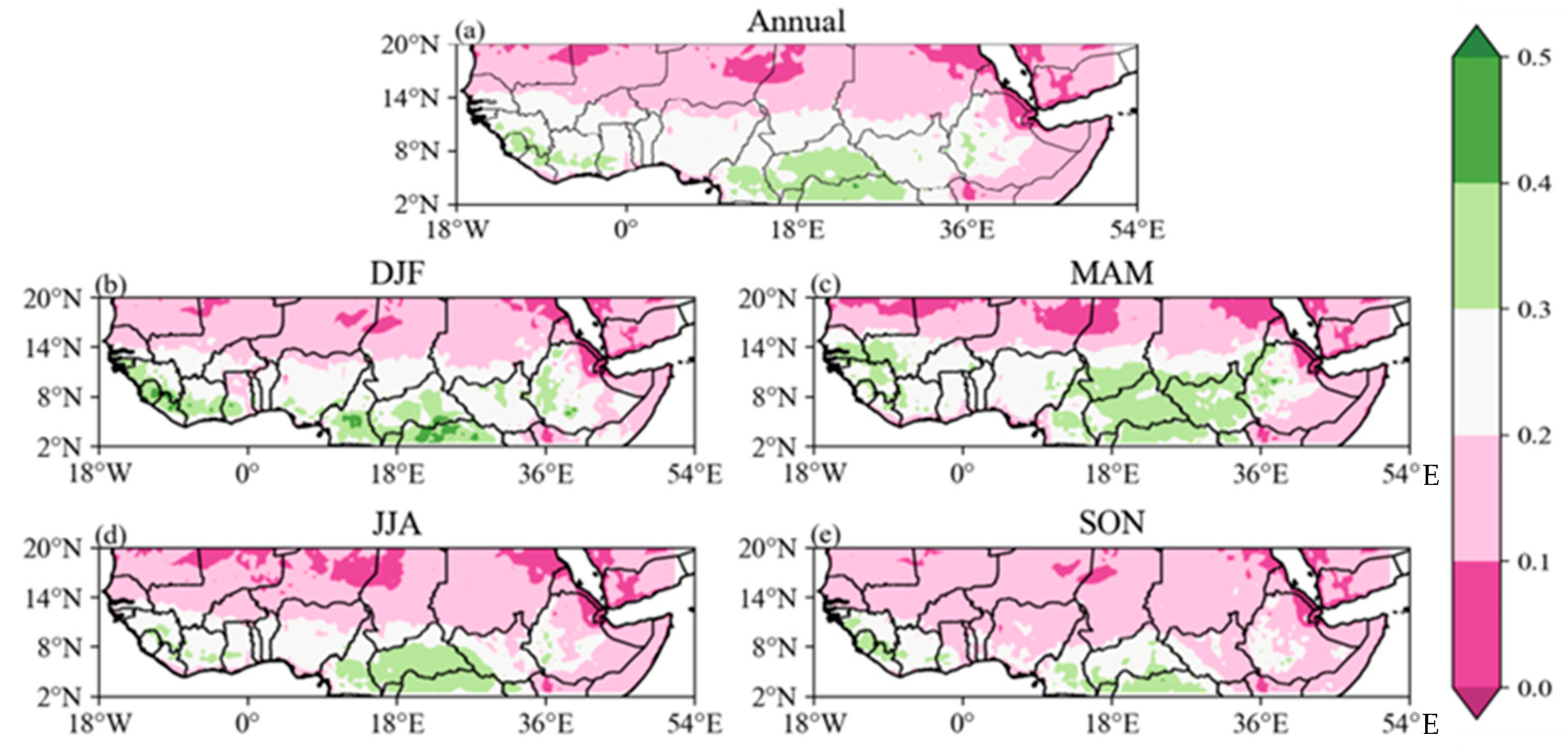
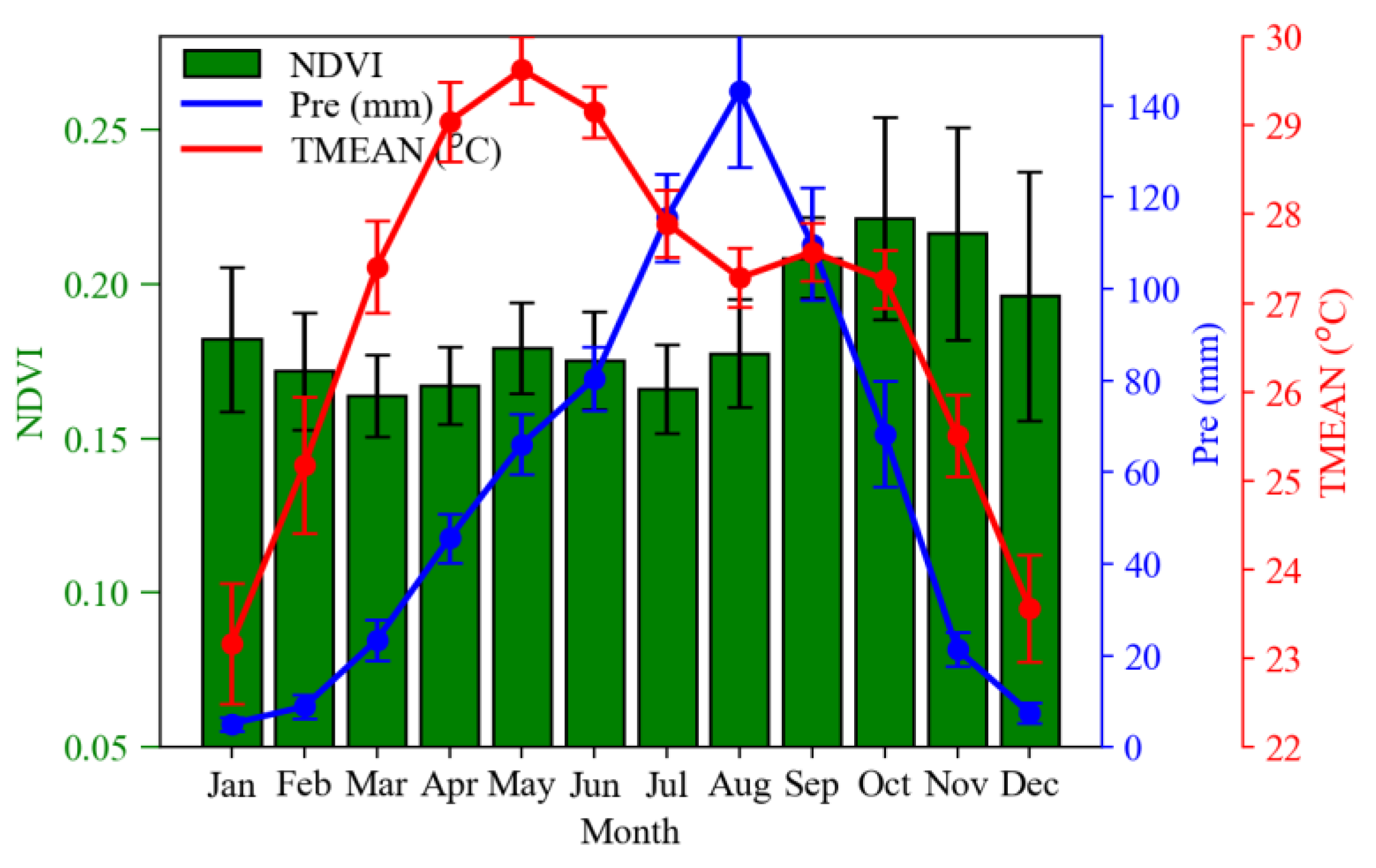
3.1. Seasonal Analysis of the NDVI

Annually, the highest NDVI values of greater than 0.5 (>0.5) are in locations 2°–8° N, 18° W–8° E and 2°–8° N, 8°–35° E, with NDVI values of 0.20–0.39 in semi-arid regions along 2°–8° N, 36–52° E and 8°–14° N. Dense vegetation canopy tends to have positive NDVI values greater than 0.4 to 0.8, which is consistent with vegetation conditions in the humid regions of the Congo Basin. Moderate NDVI values (0.2–0.35) are located in the Sahel, Savanna, GC, and southern Sudano. The lowest values of 0.1 are located in arid regions (14°–20° N). Vegetation with NDVI values < 0.1 tends to be scattered vegetation consistent with conditions in the arid regions of the Sahara Desert, Arabian Peninsula, and Horn of Africa (Figure 3a). Seasonally, the NDVI values showed similar spatial variability in the NDVI distribution, albeit with differences in the NDVI values (Figure 3b–e). Winter and spring seasons showed a similar spatial pattern in the NDVI, albeit the values differed (Figure 3b,c). The summer season showed the lowest NDVI values in arid regions of the SD, northern Sudano, ARP, and HOA. Semi-arid areas of the Sahel, Savanna, GC, and southern Sudano showed moderate values between 0.2 and 0.3 and >0.4 (Congo Basin) (Figure 3d). The autumn season showed values of >0.4 in areas in the western Savanna, Guinea Coast, and Congo Basin (Figure 3e).

The monthly NDVI values range from 0.04 to 0.22 (Figure 4, green bar). The monthly P ranges from 0 to 140 mm (Figure 4, blue line), and the TMEAN ranges from 22 to 30 °C (Figure 4, red line). All variables exhibited a clear periodic change, where the NDVI values peaked at 0.22 in October and reached their lowest value at 0.16 in July. P seasonality was highest (lowest) in August (January) at 138 (2 mm). The monthly TMEAN showed the highest (lowest) values in May (January).

3.2. Long-Term Changes in NDVI and Climate Drivers

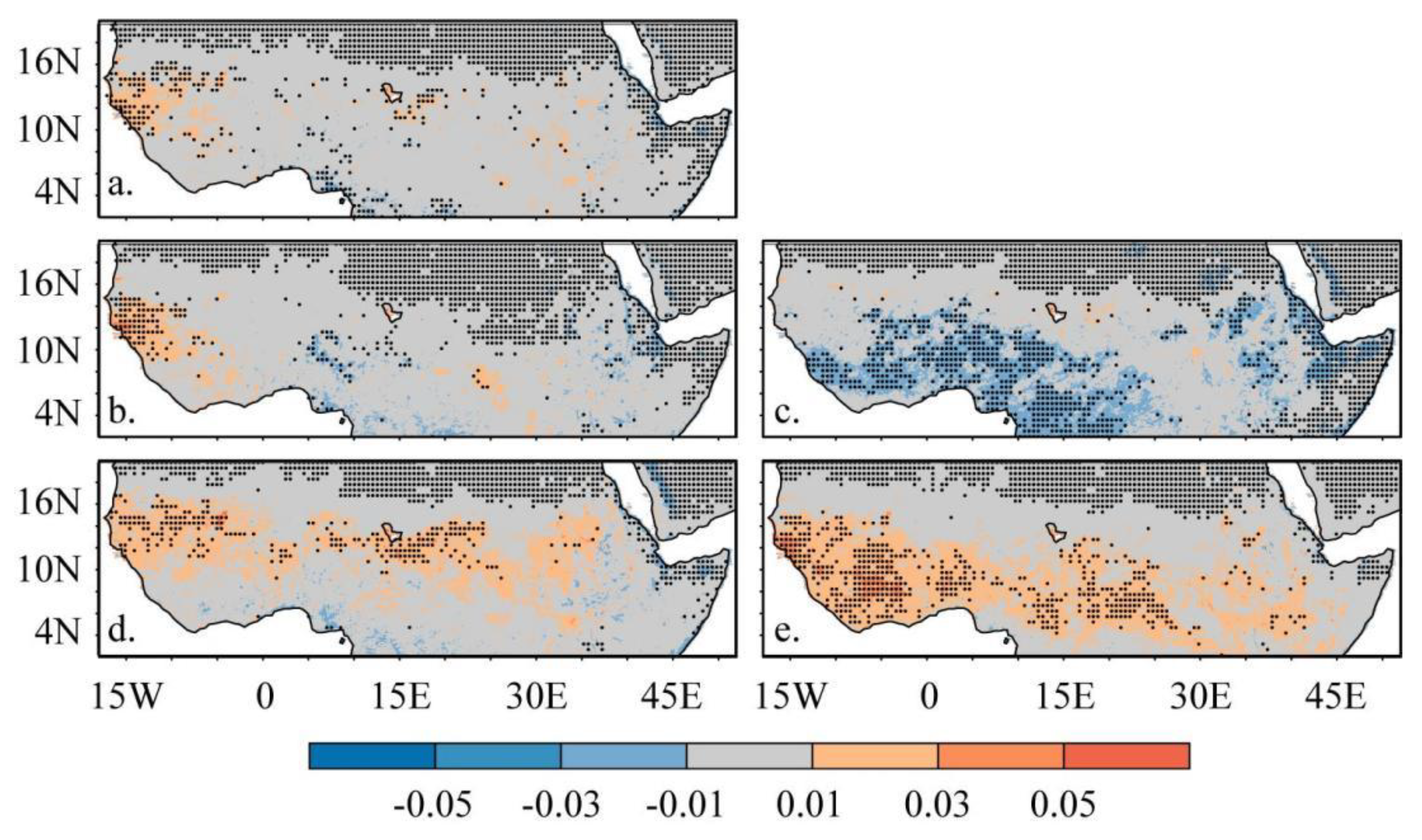
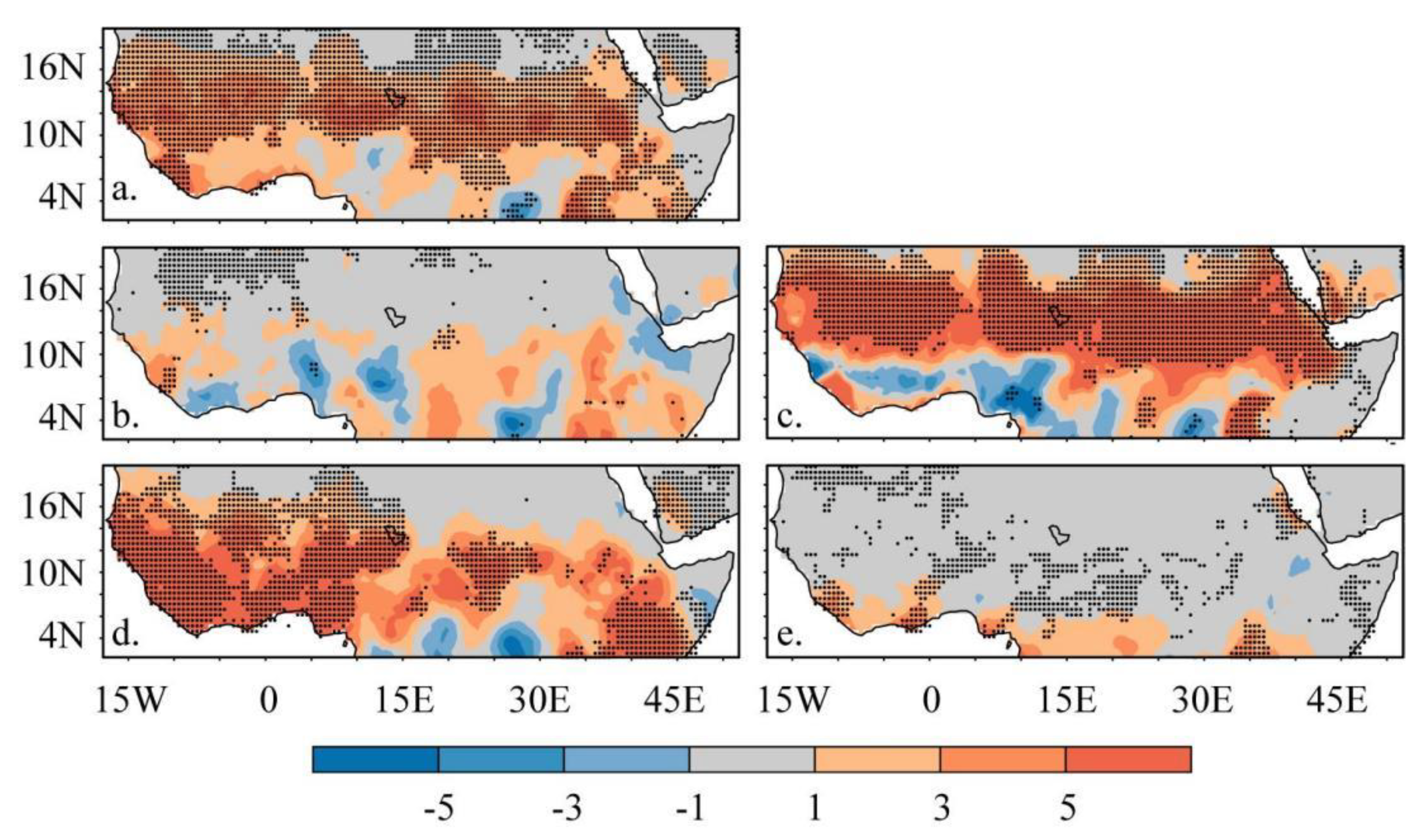
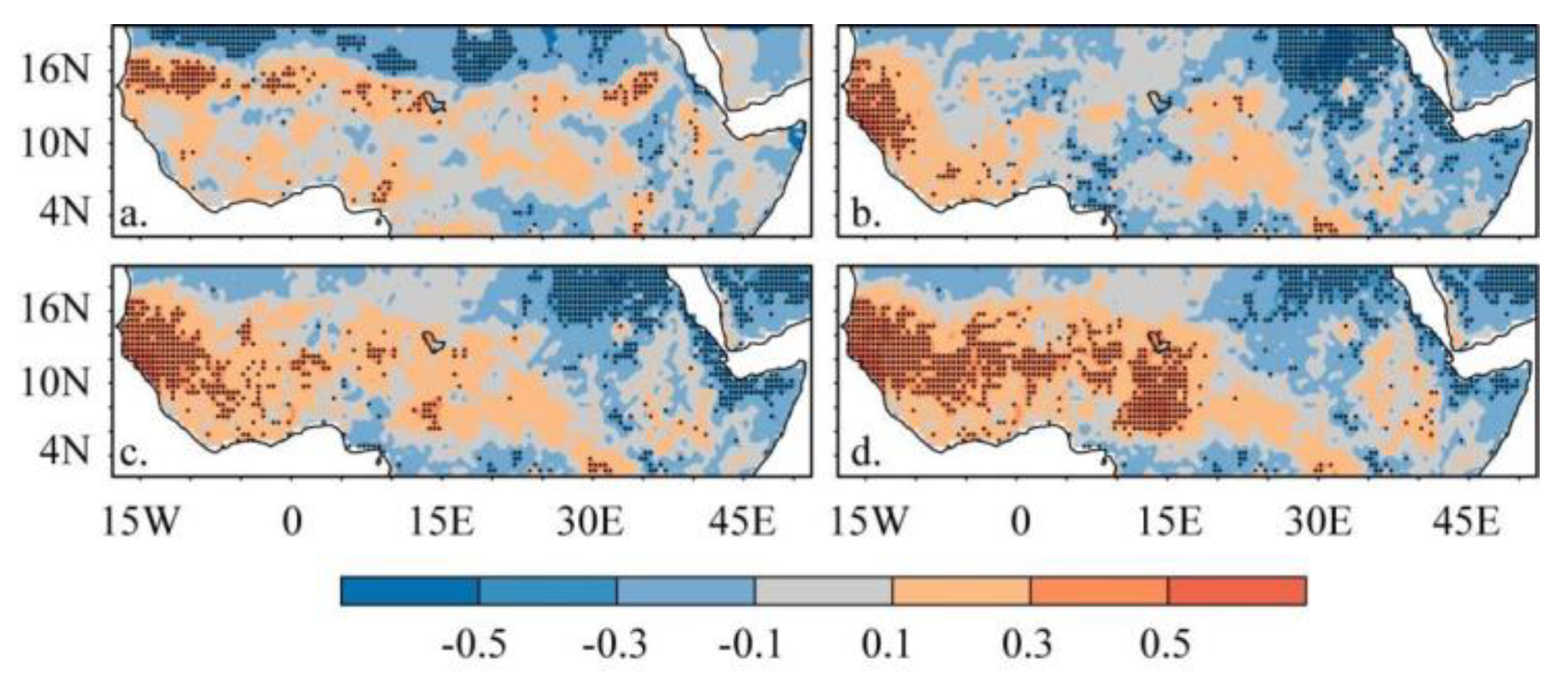
3.2.1. Spatial Trends in NDVI and Climate Drivers

The NDVI trends varied at a decadal rate of −0.5 to 0.5. However, many regions showed no significant changes in NDVI trends across the EQA region (Figure 5). The annual NDVI values exhibited an increasing trend at a rate of 0.5 per decade in the western Savanna and Sahel and in a few patches in the eastern Sahel and southern Sudano. Similarly, the annual NDVI values exhibited patches with a significant negative trend scattered along the eastern Guinea Coast, Congo Basin, and the tip of the HOA at a rate of 0.1 per decade (Figure 5a). The seasonal NDVI trends range from 0.1 to 0.5 per decade and are presented in Figure 5b–e. The spring NDVI results showed mixed trends similar to the spatial pattern of annual NDVI trends, albeit with differences in trend values (Figure 5b). Summer showed widespread, significantly decreasing NDVI trends at 0.3 per decade in areas along the Guinea Coast, eastern Savanna, and Congo Basin (Figure 5c). Autumn (Figure 5d) and winter (Figure 5e) exhibited a similar increasing trend at 0.5 per decade along the Sahel. However, the winter season showed increasing NDVI trends extending to the Savanna, Guinea Coast, Congo Basin, southern Sudano, and patches scattered in the HOA (Figure 5e).

The linear trend in P ranges from −5 to +5 mm per decade, as shown in Figure 6. Annually, P showed significant increasing trends in the Sahel, Savanna, Sudano, and HOA. The central Guinea Coast areas showed positive trends at 1 mm per decade but were insignificant (p < 0.05). The spring season showed no significant P trends (Figure 6b). The P trends during the summer presented similar values to annual P trends, except the Guinea Coast showed significant decreasing trends (Figure 6c). Similarly, the spatial pattern of P trends in autumn was identical to the annual P trends (Figure 6d, SON). The winter season showed significantly increasing P trends along the Guinea Coast and patches in the Congo Basin (Figure 6e).

The annual TMEAN ranged from −0.5 to +0.5 °C and increased across the study area (Figure 7a). Areas in the Guinea Coast, central Sahel, Congo Basin, western Sahel, northern Sudano, and parts of the HOA increased at a rate of 0.3–0.5 °C (Figure 7a, year). Generally, the spatial patterns of TMEAN trends during the spring (Figure 7b, MAM) and winter (Figure 7e, DJF) seasons were identical to annual trends. Summer trends showed that the TMEAN increased at 0.1 °C per decade along the periphery of the EQA region (Figure 7c). During the autumn season, a significantly increasing trend at 0.3 °C is widespread across the area (Figure 7d). A similar trend analysis was shown for the TMIN (Figure S1) and TMAX (Figure S2). However, in the EQA region, the TMIN exhibited more pronounced warming trends than the TMAX.

3.2.2. Temporal Trends in NDVI and Climate Drivers

Figure 8 presents the annual and seasonal variability in the NDVI and climate variables (i.e., precipitation and temperature) from 1982 to 2021.

Table 1. The slope of the annual and seasonal NDVI and meteorological variables from 1982 to 2021 over the EQA region.

Variable	Time Scales
	Annual	MAM	JJA	SON	DJF
NDVI	m = −2.3 × 10−4, c = 0.19, (α = 0.097)	m = −3.9 × 10−4, c = 0.18, (α = 0.259)	m = −7.5 × 10−4, c = 0.19, (α = 0.001)	m = 1.4 × 10−5, c = 0.22, (α = 0.478)	m = 3.3 × 10−4, c = 0.18, (α = 0.076)
P	m = 0.20, c = 55.44, (α = 0.000)	m = 0.09, c = 45.00, (α = 0.032)	m = 0.45, c = 104.66, (α = 0.000)	m = 0.34, c = 58.91, (α = 0.000)	m = 0.04, c = 6.50, (α = 0.000)
TMEAN	m = 0.02, c = 26.46, (α = 0.000)	m = 0.02, c = 28.18, (α = 0.000)	m = 0.01, c = 27.79, (α = 0.008)	m = 0.02, c = 26.32, (α = 0.000)	m = 0.03, c = 23.42, (α = 0.001)
TMAX	m = 0.02, c = 33.14, (α = 0.000)	m = 0.03, c = 35.17, (α = 0.000)	m = 0.01, c = 33.40, (α = 0.043)	m = 0.01, c = 32.89, (α = 0.001)	m = 0.03, c = 31.08, (α = 0.001)
TMIN	m = 0.02, c = 19.90 (α = 0.000)	m = 0.02, c = 21.36, (α = 0.000)	m = 0.01, c = 22.27, (α = 0.000)	m = 0.02, c = 19.95, (α = 0.000)	m = 0.02, c = 15.82. (α = 0.001)

Minus (−) value indicates a decreasing trend. α is the p-value.

illustrates the tabulated trend rate. The NDVI trends range from 0.05 to 0.30 (Figure 8a). Overall, the annual NDVI trends decreased at a decadal rate of −2.3 × 10⁻⁴ (Figure 8a, blue color). Moreover, spring (Figure 8a, orange color) and summer (Figure 8a, yellow color) showed that NDVI trends decreased at −3.9 × 10⁻⁴ and −7.5 × 10⁻⁴* year⁻¹, while the NDVI showed increasing trends of 3.3 × 10⁻⁴ and 1.4 × 10⁻⁵ year⁻¹ in autumn (Figure 8a, purple color) and winter (Figure 8a, green color), respectively. The annual P ranged from 0 to 120 mm (Figure 8b) and increased at 2.0* mm per decade from 1982 to 2021 (Table 1, P). On a seasonal scale, all four seasons showed a significant increasing trend. The summer season recorded the highest trend at 4.5 mm per decade, followed by autumn at 3.4* mm per decade. The increase in spring was 0.9 mm per decade, and winter was the lowest at 0.4 mm per decade. The average mean temperature (TMEAN) ranges from 22 °C to 30 °C (Figure 8c). The trend increased at an annual rate of 0.2* °C per decade (Table 1, TMEAN). Spring and autumn exhibited a trend rate of 0.2* °C per decade, respectively. However, the trend rate is slightly higher in winter and lowest in summer at 0.3* °C and 0.1 °C (α = 000) per decade, respectively. In addition, the TMIN and TMAX presented significantly increasing trends annually and in the four seasons, as presented in Figures S3 and S4, respectively. The TMIN ranges from 15 to 23 °C in Figure S3, and the TMAX ranges from 30 to 36 °C in Figure S4, respectively. Remarkably, all three temperature values (TMIN, TMEAN, and TMAX) exhibited an annual trend rate of 0.2* °C per decade, albeit with differences in values. At the seasonal level, the TMIN and TMEAN exhibited similar seasonal trend rates, except for the winter season, which presented rates of 0.2* °C and 0.3* °C per decade, respectively (Figure S3 and Figure 8c). On the other hand, the results of the TMAX showed a similar value of trend rate with summer and winter at 0.1 °C and 0.3* °C per decade, respectively. In spring and autumn, temperatures increased slightly to 0.31* °C and 0.1* °C per decade, respectively (Figure S4, Table 1).

The annual NDVI declined in forests and croplands at a rate of −3.0 × 10⁻³ and −0.61 × 10⁻³ and increased in shrubs and grasslands by 2.2 × 10⁻³ and 4.0 × 10⁻³ across the region from 1982 to 2021 (Figure 9). Seasonally, the NDVI declined in the forest and cropland covers conservatively in spring, summer, and autumn, except in winter, where it increased but at different rates of magnitude (Figure 9). In contrast, the NDVI increased in grassland during the spring and autumn transition seasons, except for a decline in summer. In addition, the NDVI in shrubs decreased (increased) in spring and summer (autumn and winter), albeit with different trend values.

3.3. Abrupt Change Analysis of NDVI and Climate Drivers

Table 2. The years of abrupt changes in the NDVI, P, TMEAN, TMIN, and TMAX from 1982 to 2021.

Variable	Years of Abrupt Changes
	Annual	MAM	JJA	SON	DJF
NDVI	2009	2002	2002	1994	1993
P	2002	2011	2002	1996	1988
TMEAN	2001	1997	2001	2001	1994
TMIN	2001	2000	2001	2001	2001
TMAX	2000	1997	2001	2000	1994

presents breakpoint changes for the NDVI and climate variables from 1982 to 2021. Overall, the breakpoint results showed considerable similarities and differences over the period. On the inter-annual scale, the NDVI, P, TMEAN, TMIN, and TMAX breakpoints varied and occurred at different years. The annual NDVI breakpoints were observed in 2009. For the different seasons, the spring and summer NDVI breakpoints occurred in spring and summer in 2002, while the autumn and winter breakpoints occurred in 1994 and 1993, respectively. The annual precipitation (P) breakpoint occurred in 2002 and seasonally, except in summer, which exhibited an identical breakpoint as the annual; the rest occurred in 2011 for spring, in 1996 for autumn, and winter in 1998. In the temperature values, the annual breakpoint for the TMEAN and TMIN was observed in 2001, while the TMAX occurred in 2000. Seasonally, the TMIN showed that summer and autumn had similar breakpoints in 2001, while the spring breakpoints occurred in 2000.

An analysis of the trend slope before and after the breakpoint was performed (

Table 3. The trends in the abrupt changes before and after for the NDVI, P, TMEAN, TMIN, and TMAX from 1982 to 2021.

Trends before Abrupt Changes
Variable	Annual	MAM	JJA	SON	DJF
NDVI	0.005	0011 *	0.0005	−0.0006	−0.0018
P	0.3645 *	−0.0339	0.7566 *	0.5653	0.4220
TMEAN	0.0114	−0.0021	−0.0060	0.0053	−0.0009
TMIN	0.0065	0.0058	−0.0063	0.0055	0.0193
TMAX	0.0151	0.0026	−0.0057	0.0029	−0.0033
Trends after Abrupt Changes
Variable	Annual	MAM	JJA	SON	DJF
NDVI	−0.0013	0.0006	0.0006	0.0009 *	0.0015 *
P	0.4830 *	1.6933	0.9599 *	0.5658 *	0.0835 *
TMEAN	0.0114	0.0033	−0.0060	0.0055	0.0394 *
TMIN	0.0065	−0.0066	−0.0063	0.0053	0.0193
TMAX	0.0186	0.0044	−0.0057	0.0079	0.0476 *

* Asterisk significance level at p < 0.05.

). The annual NDVI breakpoint displayed a positive (0.005) value before 2009 and a negative value after 2009, indicating that the NDVI trends were not monotonic across the EQA region from 1982 to 2021 as shown in Table 3. Seasonal analysis showed that the NDVI values exhibited positive trends in the spring before and after the breakpoint. The summer (JJA) NDVI values showed a positive trend before and after the breakpoints. The autumn and winter NDVI trends were negative before and positive after the breakpoints, respectively. For precipitation (P) analysis of trend estimates, we observed a significant positive annual trend before (0.3645) and after (0.4830) the breakpoint in 2009 (p < 0.05). Spring P exhibited positive values before and after the negative breakpoints. Summer, autumn, and winter P showed positive trends before and after the breakpoints. In addition, the TMEAN and TMIN showed no significant change in annual trends before and after the 2001 breakpoints. The TMIN, TMEAN, and TMAX exhibited positive trends before and after the spring, autumn, and winter breakpoints. In contrast, the TMIN, TMEAN, and TMAX showed negative trends before and after the breakpoints in the summer season.

3.4. Analysis of Factors That Drive NDVI Changes

Correlation Analysis of NDVI and Climate Drivers

The annual correlation coefficient (r) between the NDVI and climate factors shows R values ranging between −0.50 and +0.50 (Figure 10). Spatially, a strong positive correlation (r > 0.5, p < 0.05) was found in the Sahel and northern Sudano regions, and a negative correlation was observed in the SD and ARP (R > 0.45) between the NDVI and P (Figure 10a). However, mixed results of weak relationships (r ≤ 0.30) were found in the Savanna, Guinea Coast, and Congo Basin. Figure 10b (NDVI-TMIN) shows that strong and significant positive r ≥ 0.5 correlations mainly occurred in the western Sahel and Guinea Coast, while a weakly insignificant correlation was found in areas of southern Sudano (r ≤ 0.30, p > 0.05). The spatial patterns of positive and negative correlation trends in Figure 10c (NDVI-TMEAN) and Figure 10d (NDVI-TMAX) present similar values, with differences in magnitudes. However, the spatial patterns of positive and negative correlation trends in Figure 10c (NDVI-TMEAN) and Figure 10d (NDVI-TMAX) are identical. Seasonally, a strong relationship between the NDVI and P was observed, and this spatial pattern is comparable to spring–summer–autumn in the Sahel, Savanna, and Guinea Coast. However, the spatial patterns of r values between the NDVI and the temperature values (TMIN, TMEAN, and TMAX) were comparable to the spring and summer seasons across the region (Figure S5).

We analyzed the spatial patterns of time lag correlation to assess the time lag effects of the NDVI as responses to precipitation and temperature at the time lags of 1, 2, 3, 6, 9, and 12 months.

Table 4. The time lag correlation coefficients between the NDVI and P and T from 1982 to 2021.

Time Lag	Lag-Corr (NDVI, TMIN)	Lag-Corr (NDVI, TMEAN)	Lag-Corr (NDVI, TMAX)	Lag-Corr (NDVI, P)
1	−0.27	−0.27	−0.27	−0.21
2	−0.43	−0.42	−0.34	−0.33
3	−0.43	−0.39	−0.27	−0.35
6	−0.006	+0.11	0.28	−0.23
9	−0.32	+0.29	+0.20	+0.27
12	+0.14	+0.06	−0.07	+0.29

Note: A correlation coefficient (r) value ranges from −1 to +1. A minus sign indicates a negative correlation, and a plus sign indicates a positive correlation.

presents the time lag correlation coefficients between the NDVI and P and T from 1982 to 2021. Overall, the time lag of the NDVI negative correlation coefficients of the NDVI with responses to climatic factors differed with R values ranging from −0.6 to +0.6 over 1 to 3 months (Table 4), which signifies that the NDVI response to climate varies within 1 to 3 months, specifically the maximum and mean temperatures. Meanwhile, the TMIN leads the NDVI for up to 9 months, while the P leads the NDVI for up to 6 months. The response of the NDVI to these climate factors varied from 1 to 9 months. It can be seen that from the 12th month, the climate variables mostly lead to the NDVI. The spatial distribution of the time lag correlation is provided in Figure A1, Figure A2, Figure A3 and Figure A4 at the annual scale for the time lags for 1, 2, 3, 6, 9, and 12 months. Although significant positive correlations were found in the study area, negative correlations of the NDVI with climatic factors were observed in certain areas. This explains the heterogeneous response of the vegetation cover to climatic conditions (Figure A1, Figure A2, Figure A3 and Figure A4).

We performed a partial correlation analysis to clarify the factors driving temporal dynamics in the NDVI. Overall, the PCC results of the NDVI–climate relationship indicate that the TMIN and P results were statistically significant at p < 0.05 (

Table 5. The partial correlation coefficients between the NDVI and P and T (i.e., TMIN and TMAX) from 1981 to 2021.

Climate Factors	NDVI
P	−0.19 *
TMIN	−0.45 *
TMAX	+0.31

Note: A higher PCR value infers a greater effect and, hence, the main driving factor. A minus sign indicates the factor suppresses vegetation growth, and a plus sign encourages vegetation growth. The asterisks indicate significance at p < 0.05.

). The TMIN showed moderate negative PCC with the NDVI (R = −0.45, p < 0.05), followed by P with low negative PCC (R = −0.19, p < 0.05). This result suggests that the TMIN was the main driver that moderately influenced the NDVI during the study period.

4. Discussion

This study investigated the long-term record of vegetation dynamics and main drivers across the Equatorial Africa (EQA) region based on the annual and seasonal scale. The spatiotemporal distribution of vegetation and climate were analyzed. Trend analysis was used to analyze the spatial heterogeneity and the dynamic variations in vegetation growth and climate. In addition, correlation (partial) analysis was used to analyze the relationship between vegetation growth and climate and the driving factors. The spatial patterns in the NDVI are highly seasonal and exhibit contrasting seasonal patterns. Forests dominate the Guinea Coast, and the Congo Basin region exhibits higher NDVI values. The Sahel, Sudano, and Savanna areas are semi-arid and dominated by shrub woodlands, grasslands, and crops exhibiting high values. In contrast, areas in the Sahara Desert, Arabian Peninsula, and parts of the Horn of Africa are arid and dominated by sparse shrubs, crops, and grasslands. Overall, the vegetation pattern and its seasonal distribution suggest that changes in vegetation productivity depend on season and location, which is related to climate (e.g., precipitation and temperature).

The distribution across the region has been confirmed in previous studies [15,31,61], suggesting that vegetation trends are increasing and decreasing in different areas worldwide [62]. Some studies found that vegetation increased while others declined [63,64]. Our study found that the vegetation trends displayed spatial heterogeneity, and the overall trend slightly declined from 1992 to 2021. Previous global studies have also reported that global average temperature and changing precipitation regimes are expected to alter moisture conditions in various global land regions [9]. Our results showed that the trend in the mean average temperature increased in agreement with past studies [9]. Increasing minimum and maximum temperatures contributed to increasing mean average temperatures, which is consistent with Meehl et al. [65]. Increasing minimum temperatures are related to vapor pressure feedback, while maximum temperatures are related to local conditions such as soil moisture [66,67]. In addition, our precipitation results exhibited an increasing trend in the semi-arid regions. In contrast, mixed trends are present in the humid regions, and there was no change in precipitation in the arid regions. Our analyses of the temporal trend changes to detect the timing and significance of changes in vegetation and climate drivers showed that the breakpoint years occurred and shifted at different years consistent with past studies [68] and the reasons that drive changes require further analysis. However, there seems to be a general agreement that in parts of the study area, such as the Sahel and Sudano regions, natural climate variability influences these changes more than human-related activities, as reported by Fensholt and Rasmussen [69].

Regarding the GIMMS NDVI observations, previous global studies have reported vegetation greening in the Northern Hemisphere (NH) [70]. Other studies have reported that greening has stalled or reversed [63,70,71,72]. Our results showed spatial vegetation heterogeneity as the different regions exhibited distinct vegetation variations in browning, greening, or stagnation. Our results showed that the vegetation trend increased in the western Savanna, Sahel, and parts of Sudano. These locations are dominated by shrubs, grasses, crops, and woodlands, and the climate zone is considered semi-arid [73,74]. Furthermore, this study showed that greening along the Sahel region is consistent with Zhao et al. [62] compared with global research that reported greening in the northern hemisphere [75]. In addition, stagnant or no change in vegetation activity suggests that vegetation transitioning stalled predominately forested areas along the Guinea Coast and Congo Basin, and the region’s climate is considered a humid zone [73,74]. Likewise, vegetation transitioning stalled in the southern Sahara Desert, northern Sudano, Arabian Peninsula, and parts of the HOA. The region is arid, dominated by grasslands, crops, and sparse woodlands [73,74]. Our results of vegetation stalling are consistent with previous studies on arid and humid regions by Zhou et al. [10] and arid regions by Berdugo et al. [28]. Generally, changes in vegetation productivity are constrained by water and energy availability. Most global and regional studies have reported that wet regions are becoming wetter and drier areas are becoming drier [76,77]. Moreover, other global and regional studies have reported that watersheds can be water-limited or energy-limited to drive vegetation growth. In semi-arid regions, water-limited and energy-limited conditions dominate the constraints on woody foliage production [15,31,61]. Our results provide data on the semi-arid areas in the Sahel and Sudano regions, which show strong warming and wetting trends. Thus, it is unsurprising that the greening in these semi-arid regions is consistent with strong significant wetting, and the significantly weak warming trends in this study are consistent with previous research [15,31].

Previous global and regional studies have indicated that external climate factors influence vegetation changes [78]. Some studies reported that greening patterns are related to increasing temperature and precipitation [78]. Other studies have found that certain regions have stalled or even reversed due to changes in precipitation and temperature seasonality [63]. In this study, our correlation analysis showed spatial heterogeneity. Vegetation changes in the semi-arid region of the Sahel and major parts of the Savanna areas are strongly positively related to precipitation. Biasutti et al. [61] found that rainfall recovery in the Sahel supports foliage production. The analysis in the arid regions revealed a significant negative relationship between precipitation and vegetation, suggesting vegetation activity is significantly constrained by water conditions. The seasonal analysis of autumn precipitation correlated most significantly with vegetation change. Generally, the investigation showed that temperature values (minimum, average, and maximum) are significantly positive in the western Sahel and Savanna areas, whereas a significantly negative correlation is obvious in the northern Sudano and Arabian Peninsula. Semi-arid regions in the Sahel and western Savanna demonstrate that the area is a hot spot for land–atmosphere interactions [39,79].

We further analyzed the time lag effects of the NDVI response to the different climate factors, considering monthly values of 1 to 3 months and 6, 9, and 12 months (Appendix A, Figure A1, Figure A2, Figure A3 and Figure A4). The subregions exhibited distinct inter-annual lags in vegetation response to temperature and precipitation variations. Overall, there was a significant time-lagged effect of climate factors on vegetation growth in general, with a lag of up to three months, after which the response decreased in correlation values in line with previous studies [80,81]. Similarly, minimum temperature and precipitation primarily affect vegetation growth responses. However, the response is negative based on the partial correlation coefficients. This indicates that precipitation inhibits vegetation growth because higher precipitation generally means lower temperatures. Understanding the mechanisms by which vegetation changes occur is challenging, and future studies should explore the combined effect of natural climate variability and human activities on changing vegetation dynamics. Our findings on climate drivers emphasize that regional vegetation changes can better capture specific patterns and dynamics.

5. Conclusions

This study investigated the spatiotemporal variations in the NDVI to examine the responses of vegetation to climate and environmental factors in the EQA region using trend analysis, abrupt change, correlation (partial) analysis, and MLR at annual and seasonal scales from 1982 to 2021. The following conclusions were drawn based on our findings:

• The NDVI annual trends revealed a distinct spatial heterogeneity with obvious contrasting seasonal patterns in the Sahel, Savanna, Guinea Coast, Congo Basin, Sudano, Horn of Africa, Saharan Desert, and Arabian Peninsula at a rate of 0.5 per decade. Precipitation annual trends showed significant increasing trends in the Sahel, Savanna, Sudano, and western Guinea Coast at 0.1 mm per decade. Over the whole of the study area, the spatial patterns of the TMAX, TMIN, and TMEAN showed comparable positive trends at the annual rate of 0.2 °C per decade over the past 39 years;
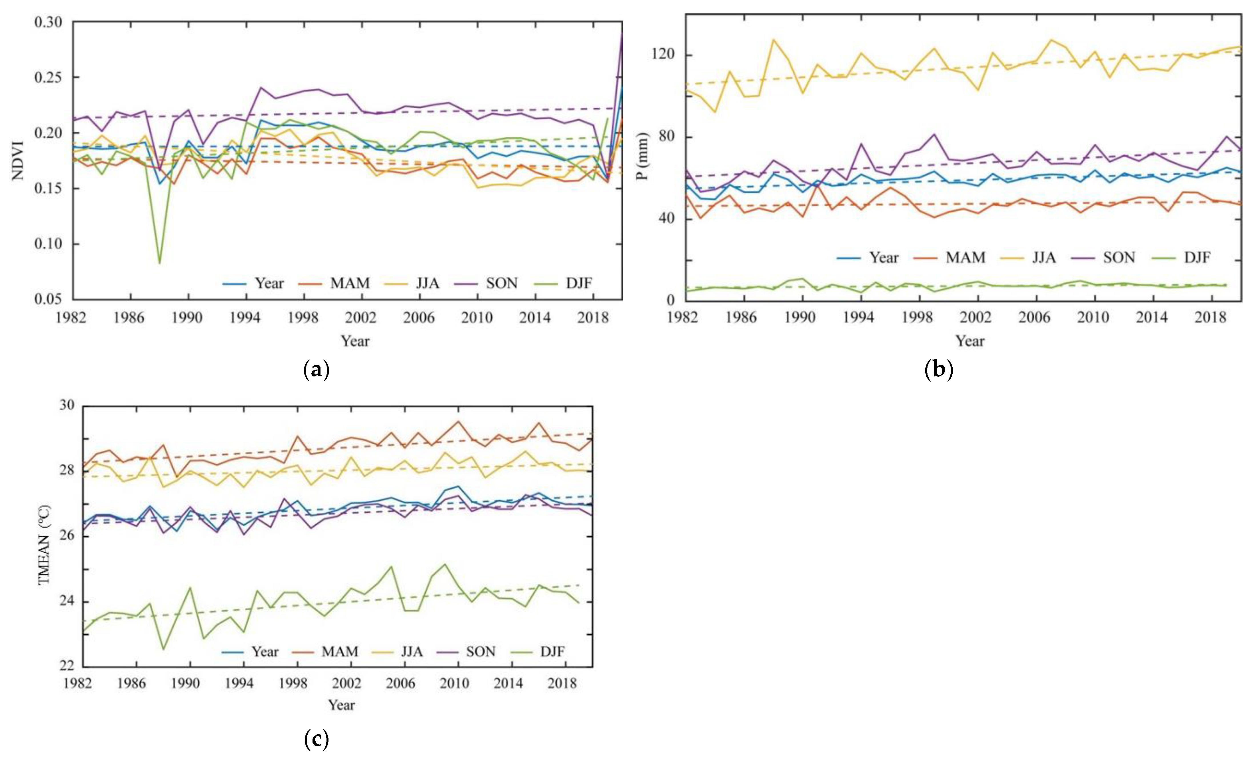
• The temporal NDVI trends decreased at an annual rate of −2.3 (×10⁻⁴) per decade, with trends decreasing in spring and summer and increasing in autumn and winter, i.e., −3.9 (×10⁻⁴) and −7.5 (×10⁻⁴); 3.3 (×10⁻⁴) and 1.4 (×10⁻⁴), respectively. Precipitation trends increased annually at a rate of 2.0 mm per decade and in all four seasons with rates of 4.5 mm10a⁻¹, 3.5 mm10a⁻¹, 0.9 mm10a⁻¹, and 0.4 mm10a⁻¹. The TMAX, TMIN, and TMEAN showed similar increasing annual trends at 0.2 °C (10a⁻¹) and in all four seasons;
• The timing of the abrupt changes differed among the NDVI, P, and TMAX (i.e., 2009, 2002, and 2000), respectively, except for the TMIN and TMEAN in 2001. The NDVI breakpoints in spring and summer occurred in 2002 but differed in autumn (1994) and winter (1993). Seasonal P timing of abrupt changes differed in all four seasons (i.e., spring, summer, autumn, and spring), occurring in 2011, 2002, 1996, and 1998, respectively. The timing of abrupt changes between the TMAX and TMIN differed in spring (1997, 2000), summer and autumn (2000, 2001), and winter (1994, 2001), respectively, except in summer in 2001;
• The annual trend showed that areas with significant greening were consistent with stronger wetter and weaker warming trends and vice versa. Spatially, summer and winter showed seasonal reversals in vegetation greening and browning trends, respectively. The spring and autumn transition seasons showed similar spatial trend patterns;
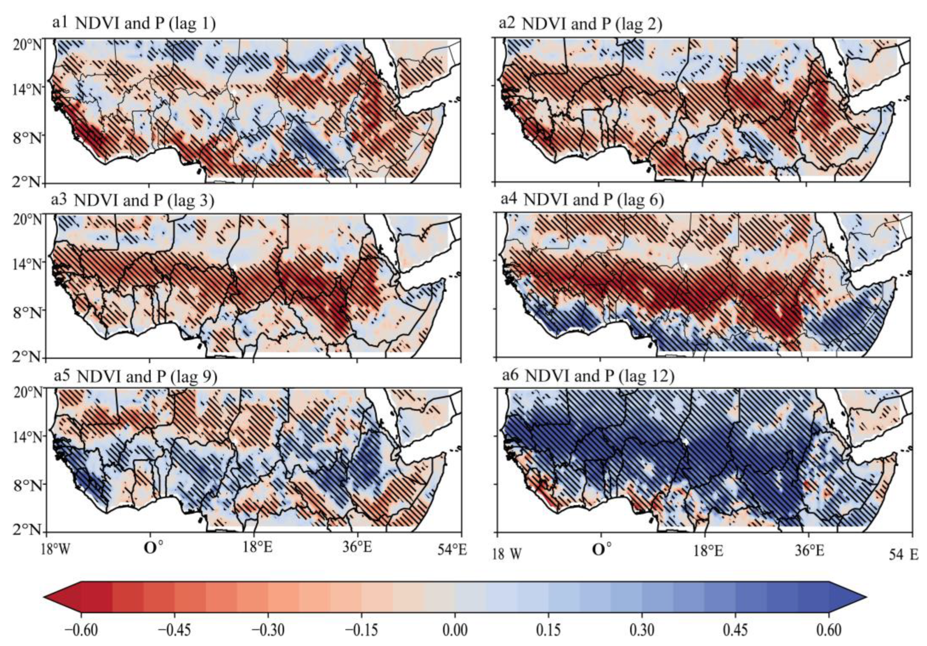
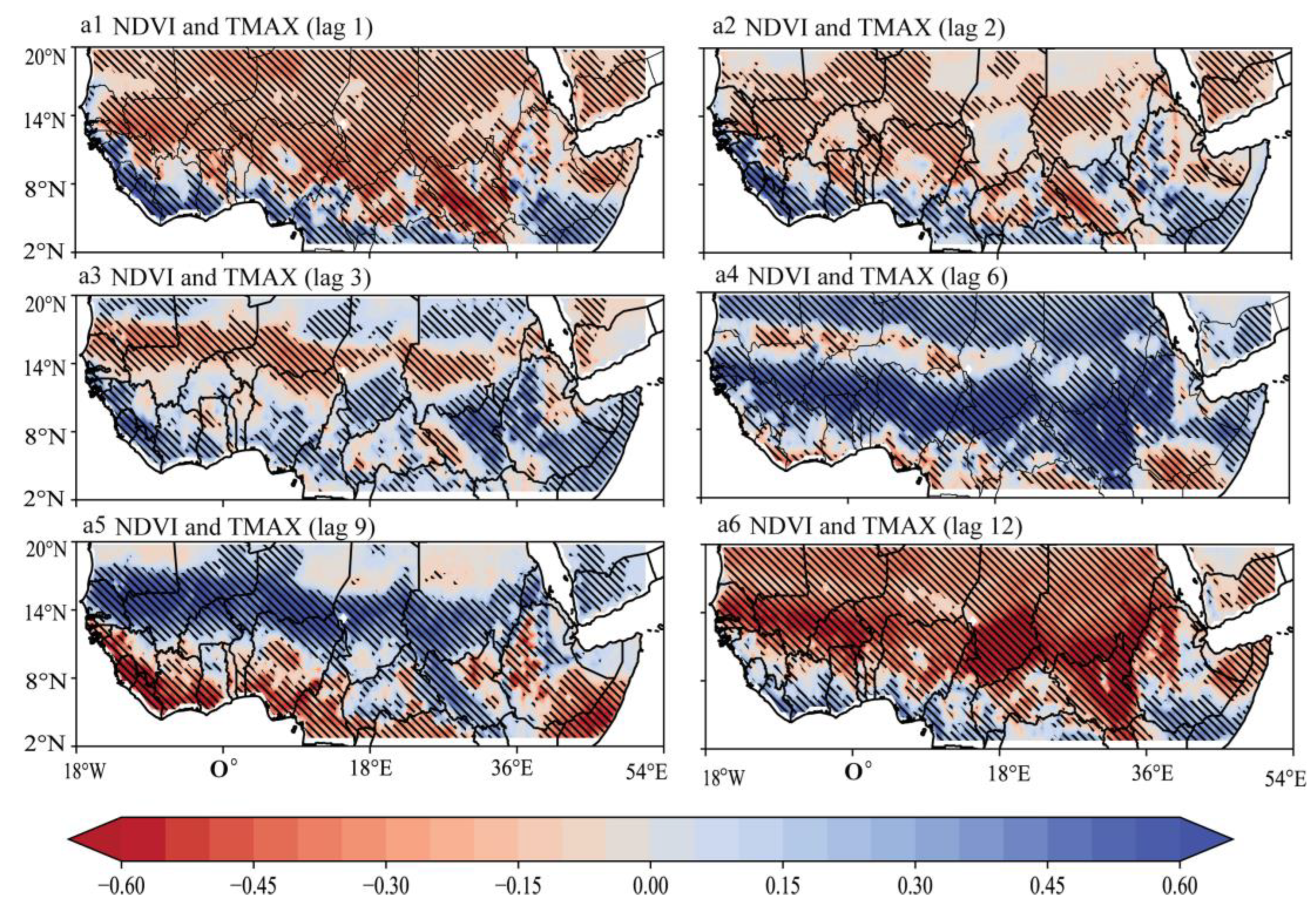
• The relationship between the NDVI and precipitation is significantly positive in the Sahel, western Savanna, and Guinea Coast and negative in the Congo Basin, Sudano, Horn of Africa, Saharan Desert, and Arabian Peninsula. Similarly, the NDVI and temperature trends showed a significant positive relationship with temperature values (TMIN, TMEAN, and TMAX) in most of the Sahel, Savanna, and Guinea Coast areas and a negative relationship with temperature in the Congo Basin, Sudano, Horn of Africa, Saharan Desert, and Arabian Peninsula. Across the study area, partial correlation analysis showed that vegetation growth response to climate variables was significant in precipitation and minimum temperature; however, the response was negative.

References

1. Zeng, J.; Zhang, Q.; Zhang, Y.; Yue, P.; Yang, Z.S.; Wang, S.; Zhang, L.; Li, H.Y. Enhanced Impact of Vegetation on Evapotranspiration in the Northern Drought-Prone Belt of China. Remote Sens. 2023, 15, 221. [Google Scholar] [CrossRef]
2. Liu, X.; Sun, G.; Fu, Z.; Ciais, P.; Feng, X.; Li, J.; Fu, B. Compound droughts slow down the greening of the Earth. Glob. Chang. Biol. 2023, 29, 3072–3084. [Google Scholar] [CrossRef] [PubMed]
3. Zhang, J.; Wu, H.Q.; Zhang, Z.; Zhang, L.L.; Luo, Y.C.; Han, J.C.; Tao, F.L. Asian Rice Calendar Dynamics Detected by Remote Sensing and Their Climate Drivers. Remote Sens. 2022, 14, 4189. [Google Scholar] [CrossRef]
4. Terasaki Hart, D.E.; Yeo, S.; Almaraz, M.; Beillouin, D.; Cardinael, R.; Garcia, E.; Kay, S.; Lovell, S.T.; Rosenstock, T.S.; Sprenkle-Hyppolite, S.; et al. Priority science can accelerate agroforestry as a natural climate solution. Nat. Clim. Chang. 2023, 13, 1179–1190. [Google Scholar] [CrossRef]
5. Thackeray, C.W.; Hall, A.; Norris, J.; Chen, D. Constraining the increased freqency of global precipitation extremes under warming. Nat. Clim. Chang. 2022, 12, 441–448. [Google Scholar] [CrossRef]
6. Madakumbura, G.D.; Thackeray, C.W.; Norris, J.; Goldenson, N.; Hall, A. Anthropogenic influence on extreme precipitation over global land areas seen in multiple observational datasets. Nat. Commun. 2021, 12, 3944. [Google Scholar] [CrossRef]
7. Qiao, L.; Zuo, Z.; Zhang, R.; Piao, S.; Xiao, D.; Zhang, K. Soil mositure-atmosphere coupling accelerates global warming. Nat. Commun. 2023, 14, 4908. [Google Scholar] [CrossRef]
8. Fischer, E.; Sippel, S.; Knutti, R. Increasing probability of record634 shattering climate extremes. Nat. Clim. Chang. 2021, 11, 689–695. [Google Scholar] [CrossRef]
9. Intergovernmental Panel on Climate Change. Technical Summary; Cambridge University Press: Cambridge, UK, 2022. [Google Scholar]
10. Zhou, L.; Tian, Y.; Myneni, R.B.; Ciais, P.; Saatchi, S.; Liu, Y.Y.; Piao, S.; Chen, H.; vermote, E.F.; Song, C.; et al. Widespread decline of Congo rainforest greeness in the past decade. Nature 2014, 509, 86–90. [Google Scholar] [CrossRef]
11. Boulton, C.A.; Lenton, T.M.; Boers, N. Pronounced loss of Amazon rainforest resilence since the early 200s. Nat. Clim. Chang. 2022, 12, 271–278. [Google Scholar] [CrossRef]
12. Liang, L.; Wang, Q.; Guan, Q.; Du, Q.; Sun, Y.; Ni, F.; Lv, S.; Shan, Y. Assessing vegetation restoration prospects under different environmental elements in cold and arid mountainous region of China. CATENA 2023, 226, 107055. [Google Scholar] [CrossRef]
13. Chen, C.; Park, T.; Wang, X.; Piao, S.; Xu, B.; Chaturvedi, R.K.; Fuchs, R.; Brovkin, V.; Ciais, P.; Fensholt, R.; et al. China and India Lead in greening of the world through land-use management. Nat. Sustain. 2019, 2, 122–129. [Google Scholar] [CrossRef] [PubMed]
14. Yu, Y.; Notaro, M.; Wang, F.; Mao, J.; Shi, X.; Wei, Y. Observed positive vegetation-rainfall feedbacks in the Sahel dominated by a mositure recycling mechanism. Nat. Commun. 2017, 8, 1873. [Google Scholar] [CrossRef] [PubMed]
15. Brandt, M.; Hiernaux, P.; Rasmussen, K.; Tucker, C.J.; Wigneron, J.; Diouf, A.A.; Herrmann, S.M.; Zhang, W.; Kergoat, L.; Mbow, C.; et al. Changes in rainfall distribution promote woody fiologe production in the Sahel. Commun. Biol. 2019, 2, 133. [Google Scholar] [CrossRef] [PubMed]
16. Dardel, C.; Kergoat, L.; Hiernaux, P.; Mougin, E.; Grippa, M.; Tucker, C.J. Re-greening Sahel: 30 years of remote sensing data and field observations (Mali, Niger). Remote Sens. Environ. 2014, 140, 350–364. [Google Scholar] [CrossRef]
17. Beck, H.E.; McVicar, T.R.; van Dijk, A.I.; Schellekens, J.; de Jeu, R.A.; Bruijnzeel, L.A. Global evaluation of four AVHRR–NDVI data sets: Intercomparison and assessment against Landsat imagery. Remote Sens. Environ. 2011, 115, 2547–2563. [Google Scholar] [CrossRef]
18. Pinzon, J.E.; Pak, E.W.; Tucker, C.J.; Bhatt, U.S.; Frost, G.V.; Macander, M.J. Global Vegetation Greenness (NDVI) from AVHRR GIMMS-3G+, 1981–2022. Available online: https://daac.ornl.gov/VEGETATION/guides/Global_Veg_Greenness_GIMMS_3G.html (accessed on 10 June 2024).
19. Tucker, C.J.; Pinzon, J.E.; Brown, M.E.; Slayback, D.A.; Pak, E.W.; Mahoney, R.; Vermote, E.F.; El Saleous, N. An extended AVHRR 8-km NDVI dataset compatible with MODIS and SPOT vegetation NDVI data. Int. J. Remote Sens. 2005, 26, 4485–4498. [Google Scholar] [CrossRef]
20. Gessesse, A.A.; Melesse, A.M. Chapter 8—Temporal relationships between time series CHIRPS-rainfall estimation and eMODIS-NDVI satellite images in Amhara Region, Ethiopia. In Extreme Hydrology and Climate Variability; Melesse, A.M., Abtew, W., Senay, G., Eds.; Elsevier: Amsterdam, The Netherlands, 2019; pp. 81–92. [Google Scholar]
21. Nicholson, S. On the question of the “recovery” of the rains in the West African Sahel. J. Arid Environ. 2005, 63, 615–641. [Google Scholar] [CrossRef]
22. Sultan, B.; Janicot, S.; Drobinski, P. Characterization of the diurnal cycle of the West African Monsoon around the monsoon onset. J. Clim. 2007, 20, 4014–4032. [Google Scholar] [CrossRef]
23. Lian, X.; Jeong, S.; Park, C.-E.; Xu, H.; Li, L.Z.X.; Wang, T.; Gentine, P.; Peñuelas, J.; Piao, S. Biophysical impacts of northern vegetation changes on seasonal warming patterns. Nat. Commun. 2022, 13, 3925. [Google Scholar] [CrossRef]
24. Myneni, R.B.; Keeling, C.D.; Tucker, C.J.; Asrar, G.; Nemani, R.R. Increased plant growth in the northern high latitudes from 1981 to 1991. Nature 1997, 386, 698–702. [Google Scholar] [CrossRef]
25. Ichii, K.; Kawabata, A.; Yamaguchi, Y. Global correlation analysis for NDVI and climatic variables and NDVI trends: 1982–1990. Int. J. Remote Sens. 2002, 23, 3873–3878. [Google Scholar] [CrossRef]
26. Brown, M.; Pinzon, J.; Didan, K.; Morisette, J.; Tucker, C. Evaluation of the consistency of long-term NDVI time series derived from AVHRR, SPOT-vegetation, SeaWIFS, MODIS and LandSAT ETM+ sensors. IEEE Trans. Geosci. Remote Sens. 2006, 44, 1787–1793. [Google Scholar] [CrossRef]
27. Zhu, Z.; Piao, S.; Myneni, R.B.; Huang, M.; Zeng, Z.; Canadell, J.G.; Ciais, P.; Sitch, S.; Friedlingstein, P.; Arneth, A.; et al. Greening of the Earth and its drivers. Nat. Clim. Chang. 2016, 6, 791–795. [Google Scholar] [CrossRef]
28. Berdugo, M.; Delgado-Baquerizo, M.; Soliveres, S.; Hernandez-Clemente, R.; Zhao, Y.; Gaitan, J.J.; Gross, N.; Saiz, H.; Maire, V.; Lehman, A.; et al. Global ecosystem thresholds driven by aridity. Science 2020, 367, 787–790. [Google Scholar] [CrossRef] [PubMed]
29. Lamchin, M.; Lee, W.K.; Jeon, S.W.; Wang, S.W.; Lim, C.H.; Song, C.; Sung, M. Long-term trend and correlation between vegetation greenness and climate variables in Asia based on satellite data. Sci. Total Environ. 2018, 618, 1089–1095. [Google Scholar] [CrossRef]
30. Peteet, D. Sensitivity and rapidity of vegetational response to abrupt climate change. Proc. Natl. Acad. Sci. USA 2000, 97, 1359–1361. [Google Scholar] [CrossRef] [PubMed]
31. Brandt, M.; Mbow, C.; Diouf, A.A.; Verger, A.; Samimi, C.; Fensholt, R. Ground- and satellite-based evidence of the biophysical mechanisms behind the greening Sahel. Glob. Chang. Biol. 2015, 21, 1610–1620. [Google Scholar] [CrossRef]
32. Gentine, P.; Massmann, A.; Lintner, B.R.; Hamed Alemohammad, S.; Fu, R.; Green, J.K.; Kennedy, D.; Vilà-Guerau de Arellano, J. Land–atmosphere interactions in the tropics—A review. Hydrol. Earth Syst. Sci. 2019, 23, 4171–4197. [Google Scholar] [CrossRef]
33. Ghebrezgabher, M.G.; Yang, T.; Yang, X.; Eyassu Sereke, T. Assessment of NDVI variations in responses to climate change in the Horn of Africa. Egypt. J. Remote Sens. Space Sci. 2020, 23, 249–261. [Google Scholar] [CrossRef]
34. Hoscilo, A.; Balzter, H.; Bartholomé, E.; Boschetti, M.; Brivio, P.A.; Brink, A.; Clerici, M.; Pekel, J.F. A conceptual model for assessing rainfall and vegetation trends in sub-Saharan Africa from satellite data. Int. J. Climatol. 2015, 35, 3582–3592. [Google Scholar] [CrossRef]
35. Seaquist, J.W.; Hickler, T.; Eklundh, L.; Ardö, J.; Heumann, B.W. Disentangling the effects of climate and people on Sahel vegetation dynamics. Biogeosciences 2009, 6, 469–477. [Google Scholar] [CrossRef]
36. Hickler, T.; Eklundh, L.; Seaquist, J.W.; Smith, B.; Ardö, J.; Olsson, L.; Sykes, M.T.; Sjöström, M. Precipitation controls Sahel greening trend. Geophys. Res. Lett. 2005, 32, L21415. [Google Scholar] [CrossRef]
37. Ogou, F.K.; Igbawua, T. Investigation of changes in vegetation cover associated with changes in its hydro-climatic drivers in recent decades over North Sub-Saharan Africa. Theor. Appl. Climatol. 2022, 149, 1135–1152. [Google Scholar] [CrossRef]
38. Dirmeyer, P. The terrestrial segment of soil moisture-climate coupling. Geophys. Res. Lett. 2011, 38, L16702. [Google Scholar] [CrossRef]
39. Koster, R.D.; Dirmeyer, P.A.; Guo, Z.; Bonan, G.; Chan, E.; Cox, P.; Gordon, C.T.; Kanae, S.; Kowalczyk, E.; Lawrence, D.; et al. The Second Phase of the Global Land–Atmosphere Coupling Experiment: Soil Moisture Contributions to Subseasonal Forecast Skill. J. Hydrometeorol. 2011, 12, 805–822. [Google Scholar] [CrossRef]
40. Mahecha, M.; Bastos, A.; Bohn, F.; Eisenhauer, N.; Feilhauer, H.; Hickler, T.; Kalesse-Los, H.; Migliavacca, M.; Otto, F.; Peng, J.; et al. Biodiversity and climate extremes: Known interactions and research gaps. Earth Future 2023, 12, e2023EF003963. [Google Scholar] [CrossRef]
41. Cox, D.T.C.; Maclean, I.M.D.; Gardner, A.S.; Gaston, K.J. Global variation in diurnal asymmetry in temperature, cloud cover, specific humidity and precipitation and its association with leaf area index. Glob. Chang. Biol. 2020, 26, 7099–7111. [Google Scholar] [CrossRef] [PubMed]
42. Funk, C.; Hoell, A.; Shukla, S.; Husak, G.; Michaelsen, J. The East African Monsoon System: Seasonal Climatologies and Recent Variations. In The Monsoons and Climate Change: Observations and Modeling; de Carvalho, L.M.V., Jones, C., Eds.; Springer International Publishing: Cham, Switzerland, 2016; pp. 163–185. [Google Scholar]
43. Sultan, B.; Janicot, S. Abrupt shift of the ITCZ over West Africa and intra-seasonal variability. Geophys. Res. Lett. 2000, 27, 3353–3356. [Google Scholar] [CrossRef]
44. Harris, I.; Jones, P.; Osborn, T.; Lister, D. Updated high–resolution grids of monthly climatic observations–the CRU TS3.10 dataset. Int. J. Climatol. 2014, 34, 623–642. [Google Scholar] [CrossRef]
45. Nooni, I.K.; Ogou, F.K.; Hagan, D.F.; Saidou Chaibou, A.A.; Prempeh, N.A.; Nakoty, F.M.; Jin, Z.; Lu, J. The Relationship between Changes in Hydro-Climate Factors and Maize Crop Production in the Equatorial African Region from 1980 to 2021. Atmosphere 2024, 15, 542. [Google Scholar] [CrossRef]
46. Hansen, M.C.; Defries, R.S.; Townshend, J.R.G.; Sohlberg, R. Global land cover classification at 1 km spatial resolution using a classification tree approach. Int. J. Remote Sens. 2000, 21, 1331–1364. [Google Scholar] [CrossRef]
47. de Jong, R.; de Bruin, S.; de Wit, A.; Schaepman, M.E.; Dent, D.L. Analysis of monotonic greening and browning trends from global NDVI time-series. Remote Sens. Environ. 2011, 115, 692–702. [Google Scholar] [CrossRef]
48. Holben, B.N. Characteristics of maximum-value composite images from temporal AVHRR data. Int. J. Remote Sens. 1986, 7, 1417–1434. [Google Scholar] [CrossRef]
49. Basak, D.; Bose, A.; Roy, S.; Chowdhury, I.R. Chapter 17—Understanding the forest cover dynamics and its health status using GIS-based analytical hierarchy process: A study from Alipurduar district, West Bengal, India. In Water, Land, and Forest Susceptibility and Sustainability; Chatterjee, U., Pradhan, B., Kumar, S., Saha, S., Zakwan, M., Fath, B.D., Fiscus, D., Eds.; Elsevier: Amsterdam, The Netherlands, 2023; Volume 1, pp. 475–508. [Google Scholar]
50. Zeng, Y.; Hao, D.; Huete, A.; Dechant, B.; Berry, J.; Chen, J.M.; Joiner, J.; Frankenberg, C.; Bond-Lamberty, B.; Ryu, Y.; et al. Optical vegetation indices for monitoring terrestrial ecosystems globally. Nat. Rev. Earth Environ. 2022, 3, 477–493. [Google Scholar] [CrossRef]
51. Mitchell, T.D.; Jones, P.D. An improved method of constructing a database of monthly climate observations and associated high-resolution grids. Int. J. Climatol. 2005, 25, 693–712. [Google Scholar] [CrossRef]
52. New, M.; Hulme, M.; Jones, P.D. Representing twentieth century spaceetime climate variability. Part 2: Development of 1901e96 monthly grids of terrestrial surface climate. J. Clim. 2000, 13, 2217–2238. [Google Scholar] [CrossRef]
53. Mann, H.B. Non-parametric tests against trend. Econometrica 1945, 13, 245–259. [Google Scholar] [CrossRef]
54. Kendall, M. Rank Correlation Measures; Charles Griffin: London, UK, 1975; Volume 202. [Google Scholar]
55. Sen, P.K. Estimates of the Regression Coefficient Based on Kendall’s Tau. J. Am. Stat. Assoc. 1968, 63, 1379–1389. [Google Scholar] [CrossRef]
56. Pettitt, A.N. A non-parametric approach to the change-point problem. J. R. Stat. Soc. 1979, 28, 126–135. [Google Scholar] [CrossRef]
57. Verstraeten, G.; Poesen, J.; Demaree, G.; Salles, C. Long-term (105 years) variability in rain erosivity as derived from 10-min rainfall depth data for Ukkel (Brussels, Belgium): Implications for assessing soil erosion rates. J. Geophys. Res. 2006, 111, D22109. [Google Scholar] [CrossRef]
58. Adeyeri, O.E.; Ishola, K.A. Variability and Trends of Actual Evapotranspiration over West Africa: The Role of Environmental Drivers. Agric. For. Meteorol. 2021, 308–309, 108574. [Google Scholar] [CrossRef]
59. Nooni, I.K.; Wang, G.; Hagan, D.F.T.; Lu, J.; Ullah, W.; Li, S. Evapotranspiration and its Components in the Nile River Basin Based on Long-Term Satellite Assimilation Product. Water 2019, 11, 1400. [Google Scholar] [CrossRef]
60. Akimoto, F.; Matsunami, A.; Kamata, Y.; Kodama, I.; Kitagawa, K.; Arai, N.; Higuchi, T.; Itoh, A.; Haraguchi, H. Cross-Correlation Analysis of Atmospheric Trace Concentrations of N2O, CH4 and CO2 Determined by Continuous Gas-Chromatographic Monitoring. Energy 2005, 30, 299–311. [Google Scholar] [CrossRef]
61. Biasutti, M. Rainfall trends in the African Sahel: Characteristics, processes, and causes. WIREs Clim. Chang. 2019, 10, e591. [Google Scholar] [CrossRef]
62. Zhao, L.; Dai, A.; Dong, B. Changes in global vegetation activity and its driving factors during 1982–2013. Agric. For. Meteorol. 2018, 249, 198–209. [Google Scholar] [CrossRef]
63. Wang, X.; Piao, S.; Ciais, P.; Li, J.; Friedlingstein, P.; Koven, C.; Chen, A. Spring temperature change and its implication in the change of vegetation growth in North America from 1982 to 2006. Proc. Natl. Acad. Sci. USA 2011, 108, 1240–1245. [Google Scholar] [CrossRef] [PubMed]
64. Piao, S.L.; Wang, X.H.; Ciais, P.; Zhu, B.; Wang, T.; Liu, J. Changes in satellite-derived vegetation growth trend in temperate and boreal Eurasia from 1982 to 2006. Glob. Chang. Biol. 2011, 17, 3228–3239. [Google Scholar] [CrossRef]
65. Meehl, G.A.; Stocker, T.F.; Collins, W.D.; Gaye, A.J.; Gregory, J.M.; Kitoh, A.; Knutti, R.; Murphy, J.M.; Noda, A.; Raper, S.C.B.; et al. Global Climate Projection; Cambridge University Press: Cambridge, UK; New York, NY, USA, 2007. [Google Scholar]
66. Hatfield, J.L.; Prueger, J.H. Temperature extremes: Effect on plant growth and development. Weather Clim. Extrem. 2015, 10, 4–10. [Google Scholar] [CrossRef]
67. Alfaro, E.T.; Gershunov, D.; Cayan, D. Prediction of summer maximum and minimum temperature over the central and western United States: The roles of soil moisture and sea surface temperature. J. Clim. 2006, 19, 1407–1421. [Google Scholar] [CrossRef]
68. Verbesselt, J.; Hyndman, R.; Zeileis, A.; Culvenor, D. Phenological change detection while accounting for abrupt and gradual trends in satellite image time series. Remote Sens. Environ. 2010, 114, 2970–2980. [Google Scholar] [CrossRef]
69. Fensholt, R.; Rasmussen, K. Analysis of trends in the Sahelian ‘rain-use efficiency’ using GIMMS NDVI, RFE and GPCP rainfall data. Remote Sens. Environ. 2011, 115, 438–451. [Google Scholar] [CrossRef]
70. de Jong, R.; Verbesselt, J.; Schaepman, M.E.; de Bruin, S. Trend changes in global greening and browning: Contribution of short-term trends to longer-term change. Glob. Chang. Biol. 2012, 18, 642–655. [Google Scholar] [CrossRef]
71. De Jong, R.; Verbesselt, J.; Zeileis, A.; Schaepman, M.E. Shifts in Global Vegetation Activity Trends. Remote Sens. 2013, 5, 1117–1133. [Google Scholar] [CrossRef]
72. Zhao, M.; Running, S.W. Drought-induced reduction in global terrestrial net primary production from 2000 through 2009. Science 2010, 329, 940–943. [Google Scholar] [CrossRef] [PubMed]
73. Mukherjee, S.; Mishra, A.K.; Zscheischler, J.; Entekhabi, D. Interaction between dry and hot extremes at a global scale using a cascade modeling framework. Nat. Commun. 2023, 14, 277. [Google Scholar] [CrossRef]
74. Adepoju, K.; Adelabu, S.; Fashae, O. Vegetation Response to Recent Trends in Climate and Landuse Dynamics in a Typical Humid and Dry Tropical Region under Global Change. Adv. Meteorol. 2019, 2019, 4946127. [Google Scholar] [CrossRef]
75. Piao, S.; Wang, X.; Park, T.; Chen, C.; Lian, X.; He, Y.; Bjerke, J.W.; Chen, A.; Ciais, P.; Tømmervik, H.; et al. Characteristics, drivers and feedbacks of global greening. Nat. Rev. Earth Environ. 2020, 1, 14–27. [Google Scholar] [CrossRef]
76. Zaitchik, B.F.; Rodell, M.; Biasutti, M.; Seneviratne, S.I. Wetting and drying trends under climate change. Nat. Water 2023, 1, 502–513. [Google Scholar] [CrossRef]
77. Xiong, J.; Guo, S.; Abhishek; Chen, J.; Yin, J. Global evaluation of the “dry gets drier, and wet gets wetter” paradigm from a terrestrial water storage change perspective. Hydrol. Earth Syst. Sci. 2022, 26, 6457–6476. [Google Scholar] [CrossRef]
78. Zhou, L.; Tucker, C.J.; Kaufmann, R.K.; Slayback, D.; Shabanov, N.V.; Myneni, R.B. Variations in northern vegetation activity inferred from satellite data of vegetation index during 1981 to 1999. J. Geophys. Res. Atmos. 2001, 106, 20069–20083. [Google Scholar] [CrossRef]
79. Seneviratne, S.I.; Lüthi, D.; Litschi, M.; Schär, C. Land–atmosphere coupling and climate change in Europe. Nature 2006, 443, 205–209. [Google Scholar] [CrossRef] [PubMed]
80. Vicente-Serrano, S.M.; Gouveia, C.; Camarero, J.J. Response of vegetation to drought time-scales across global land biomes. Proc. Natl. Acad. Sci. USA 2012, 110, 52–57. [Google Scholar] [CrossRef] [PubMed]
81. Anderson, L.O.; Malhi, Y.; Aragão, L.E.O.C.; Ladle, R.; Arai, E.; Barbier, N.; Phillips, O.L. Remote sensing detection of droughts in Amazonian forest canopies. New Phytol. 2010, 187, 733–750. [Google Scholar] [CrossRef] [PubMed]
Figure 1. The location of the study area. (a) Study area with subregions: (1) Sahara Desert [21°–37° N], (2) Sahel [12° N–20° N, 18° W–18° E], (3) Savanna [8° N–12° N, 18° W–18° E], (4) Guinea Coast [4–8° N, 18° W–18° E], (5) Congo Basin [2°–4° N, 18°–25° E], (6) Sudano belt [12° N–20° N, 18°–25° E], (7) Arabian Peninsula (ARP) [12°–20° N, 25°–52° E], and (8) Horn of Africa (HOA) [8°–20° N, 25°–52° E]. (b) AVHRR land cover map: ENF—evergreen needleleaf forest (0.00%), EBF—evergreen broadleaf forest (3.89%), DNF—deciduous needleleaf forest (0.00%), DBF—deciduous broadleaf forest (0.13%), MF—mixed forest (0.00%), WL—woodland (7.68%), WGL—woodland grassland (20.20%), CSL—closed shrubland (5.52%), OSL—open Shrubland (9.80%), GL—grassland (4.38%), CL—cropland (3.67%), UBU—urban and built-up, BG—barren or sparsely vegetated (27.60%), and water (17.11%). (c) Elevation.
Forests 15 01129 g001
Figure 2. The work flowchart for this study.
Forests 15 01129 g002
Figure 3. The spatial distribution of the maximum NDVI values across EQA from 1982 to 2021. (a) annual, (b) winter (DJF), (c) spring (MAM), (d) summer (JJA), and (e) autumn (SON).
Forests 15 01129 g003
Figure 4. Monthly average changes in the NDVI (green bar) and climate factors in the EQA region. NDVI—green bar; precipitation—blue line; and mean temperature—red line.
Forests 15 01129 g004
Figure 5. The spatial patterns of the NDVI trends in Equatorial Africa during 1982–2021. (a) Annual, (b) spring (MAM), (c) summer (JJA), (d) autumn (SON), and (e) winter (DJF). The blue–red legend denotes negative–positive trends. The dots in the maps denote the significant results at p < 0.05. Positive and negative changes in the NDVI are called greening and browning, respectively.
Forests 15 01129 g005
Figure 6. The spatial patterns of precipitation (P) trends. (a) Annual, (b) spring (MAM), (c) summer (JJA), (d) autumn (SON), and (e) winter (DJF). The blue–red legend denotes negative–positive trends. The dots in the maps denote the significant results at p < 0.05. Positive and negative changes in precipitation are called wetting and drying, respectively.
Forests 15 01129 g006
Figure 7. The spatial patterns of mean average temperature (TMEAN) trends. (a) Annual, (b) spring (MAM), (c) summer (JJA), (d) autumn (SON), and (e) winter (DJF). The blue–red legend denotes negative–positive trends. The dots in the maps denote the significant results at p < 0.05. Positive and negative temperature changes are called warming and cooling, respectively.
Forests 15 01129 g007
Figure 8. The inter-annual variations in (a) the mean NDVI, (b) P, and (c) TMEAN at annual and seasonal timescales from 1982 to 2021. The linear trend calculated using the linear regression (dashed lines) trend is calculated using the least squares linear trend fitting method over the period (at p-value < 0.05). Annual (blue color), spring (MAM, orange color), summer (JJA, yellow), autumn (SON, purple color), and winter (DJF, green color).
Forests 15 01129 g008
Figure 9. The temporal trends in the mean NDVI from 1982 to 2021 across EQA in four dominant vegetation types.
Forests 15 01129 g009
Figure 10. Spatial correlation analysis of the annual and seasonal NDVI with climatic variables: (a) NDVI vs. PRE, (b) NDVI vs. TMIN, (c) NDVI vs. TMEAN, and (d) NDVI vs. TMAX across EQA during 1982–2021. The blue–red legend denotes a negative–positive relationship. The dots in the maps denote the significant results at p < 0.05.
Forests 15 01129 g010