Individual Tree Identification and Segmentation in Pinus spp. Stands through Portable LiDAR

Abstract

Forest inventories are essential for sustainable forest management. In inventories at the tree level, all the information is linked to individuals: species, diameter, height, or spatial distribution, for example. Currently, the implementation of Portable LiDAR (PLS) is being studied, aiming to digitalize forest environments and increase the reliability of forest observations. Performing automatic individual tree identification (ITD) and segmentation (ITS) is essential for the operational implementation of PLS in forestry. Multiple algorithms have been developed for performing these tasks in LiDAR point clouds. Their performance varies according to the LiDAR system and the characteristics of the stand. In this study, the performance of several ITD and ITS algorithms is analyzed in very high-density PLS point clouds in Pinus species stands with a varying presence of understory, shrubs, and branches. The results showed that ITD methods based on finding trunks are more suitable for tree identification in regular stands with no understory. In the ITS process, the methods evaluated are highly conditioned by the presence of understory and branches. The results of this comparison help to identify the most suitable algorithm to be applied to these types of stands, and hence, they might enhance the operability of PLS systems.

1. Introduction

The compilation of updated information about forest stands is essential for monitoring and preserving their economic, ecological, and social functions [1,2]. For decades, data gathering for forest inventories consisted of field campaigns involving plot surveys [3]. In several countries, field-based methods are still used at a local level, and the results are also extrapolated to broader scales, either regionally or nationally [4,5]. The data collected in forest inventories commonly include the identification of every single tree in a plot [6,7]. This is necessary in order to count trees, estimate stand density, identify species at a tree level, analyze spatial distribution, and monitor temporal changes [6,8]. The identification of individual trees is also a key step that facilitates crown segmentation, which is essential for producing detailed volume and biomass estimations [9]. However, surveying the geospatial position of each individual tree through fieldwork represents a large time and financial investment. Consequently, the frequency, size, and scope of forest inventories are negatively affected [10,11]. Furthermore, data collected in the field are also affected by the inherent limitations of manual measurements, mainly inconsistency and subjectivity [12,13,14].

In recent years, LiDAR-based solutions have become widely extensive for forest applications since they provide accurate three-dimensional representations of target environments [15,16,17]. LiDAR counters many of the drawbacks of traditional approaches and has led to the enhancement of forest inventory data [13]. A variety of platforms can be used to hold LiDAR devices: aerial platforms (either manned or unmanned aerial vehicles), ground platforms (either static-like, terrestrial, or mobile laser scanners), and onboard satellite platforms [18]. Airborne laser scanning (ALS), the most commonly used system in forest applications, has limitations when it comes to performing tree-level analysis since it hardly ever provides representations of tree trunks or point densities great enough to differentiate between crowns and/or trunks in close canopy stands (i.e., positions, three-dimensional structures) [19,20]. Ground-based LiDAR systems offer a practical alternative, as they can produce very dense point clouds of the lower strata of vegetation [21,22,23]. Portable laser scanner (PLS) systems, also deemed handheld or wearable laser scanners in the scientific literature [20], are increasingly gaining attention among the community of forestry technicians. By virtue of their portability, PLS systems provide high-point cloud densities and reduce the time and costs of fieldwork. Additionally, they are not affected by the occlusion problems typical of static terrestrial laser scanners (TLS) in forest environments [21,24,25].

The first step of a stand characterization at tree level through LiDAR point clouds is individual tree identification and segmentation. The individual tree identification (ITD) process refers to finding geolocated points that represent the position of either the crown apexes or the trunk centers of all those individual trees that integrate the forest stand. Individual tree segmentation (ITS) is the process by which all the points within a point cloud that belong to a single tree, including crown, trunk, and branches, are identified. These two terms have sometimes been used indiscriminately [26,27], but they are mostly distinguished as different processes and carried out as concatenated steps: the positions of single trees are used as initial points (seeds) in the segmentation procedure; in these cases, the verification step evaluates only segmentation efficiency [8,28,29].

Performing automatic ITD and ITS is essential for the operational implementation of PLS in forestry. The most widely extended methods for performing ITD in point clouds can be grouped into two main categories: raster-based methods and point-cloud-based methods [19,30]. The most common raster-based methods assume that the local maxima (LM) values within a LiDAR-derived canopy height model (CHM) correspond to tree crown apexes. The scientific literature attests to the extensive exploration of these methods in varying stands and conditions, given their simple implementation [30]. Li et al. [29] and Popescu and Wynne [31] describe two of the most common approaches. It has been shown that the results of the LM methods are affected by tree apical dominance, canopy closure, and understory presence [32,33]. The spread of LiDAR devices mounted on ground and UAV platforms, which provide dense point clouds of the lower strata of forest stands, has led to the development of tree identification methods based on finding trunks within a three-dimensional point cloud. The most common methods are based on point-density clustering. Picos et al. [34] compared raster-based and point-cloud-based methods in a high-density UAV LiDAR point cloud. Latella et al. [26] and Solares-Canal et al. [35] developed approaches for TLS point clouds. Gollob et al. [20] compared the performance of point-cloud-based algorithms in TLS and PLS data. The main drawback of density-clustering methods is that they require long computation times, making them inefficient or ineffective in processing very high-density point clouds like those provided by PLS devices [26,36].

The ITS methods can also be grouped into raster-based and point-cloud-based methods. Raster-based methods apply image processing or computer vision techniques to CHM raster layers or digital surface models (DSMs) to determine the contour boundary of tree crowns; points identified as corresponding to the geolocated position of the tree can be used as seeds. The sensitivity of these segmentation procedures to the initial tree position has not been a common focus of study. Furthermore, several authors have pointed out that over-identification or under-identification of individuals negatively affects the quality of tree segmentation [30,37]; in most cases, however, these two phenomena are not distinguished nor evaluated separately, for example, in the studies performed by Bülbül et al. [8], Yang et al. [9] or Hu et al. [38]. According to Yang et al. [39], the most common raster-based algorithms are methods based on watersheds [38,40], regional growth [41], and template matching [42]. The review provided by Yang et al. [9] revealed that raster-based methods usually show weakness where trees tightly overlap and in multilayered stands. Point-cloud-based methods use the point cloud directly to segment single trees. The most common methods are point clustering [43] and voxel-based methods [44]. Several studies serve to compare varying approaches across the different types of Laser Scanning technology: Vauhkonen et al. [27] and Zaforemska et al. [33] in ALS, Burt et al. [45], Fu et al. [46] in TLS, and Tockner et al. [37] in PLS. In general, point-cloud-based methods are more accurate for segmentation than raster-based methods [19]. However, they are complex and show poor generalizability or low efficiency in complex stands [47].

Considering the multiple algorithms that can be used in ITD and ITS, further studies are needed to evaluate their performance when applied to PLS point clouds in stands with different species and structures since these factors determine their performance [19,32,33,47,48]. Studies comparing different algorithms’ performance in the same stand would be useful for technicians to select the most appropriate algorithm to be applied in each situation.

In this study, the performance of several ITD and ITS algorithms is analyzed in very high-density point clouds obtained through PLS in Pinus species stands with moderate apical dominance and a varying presence of understory, shrubs, and branches. Raster-based and point-cloud-based methods are compared, including some common treetop and trunk detection approaches. The efficiency of both ITS and ITD processes is evaluated, including a sensibility analysis of the ITS results to the ITD points that are used as initial seeds. The study is accomplished in plots of P. pinaster and P. radiata, the most common Pinus species in Galicia, a region that concentrates 50% of the Spanish forest harvestings.

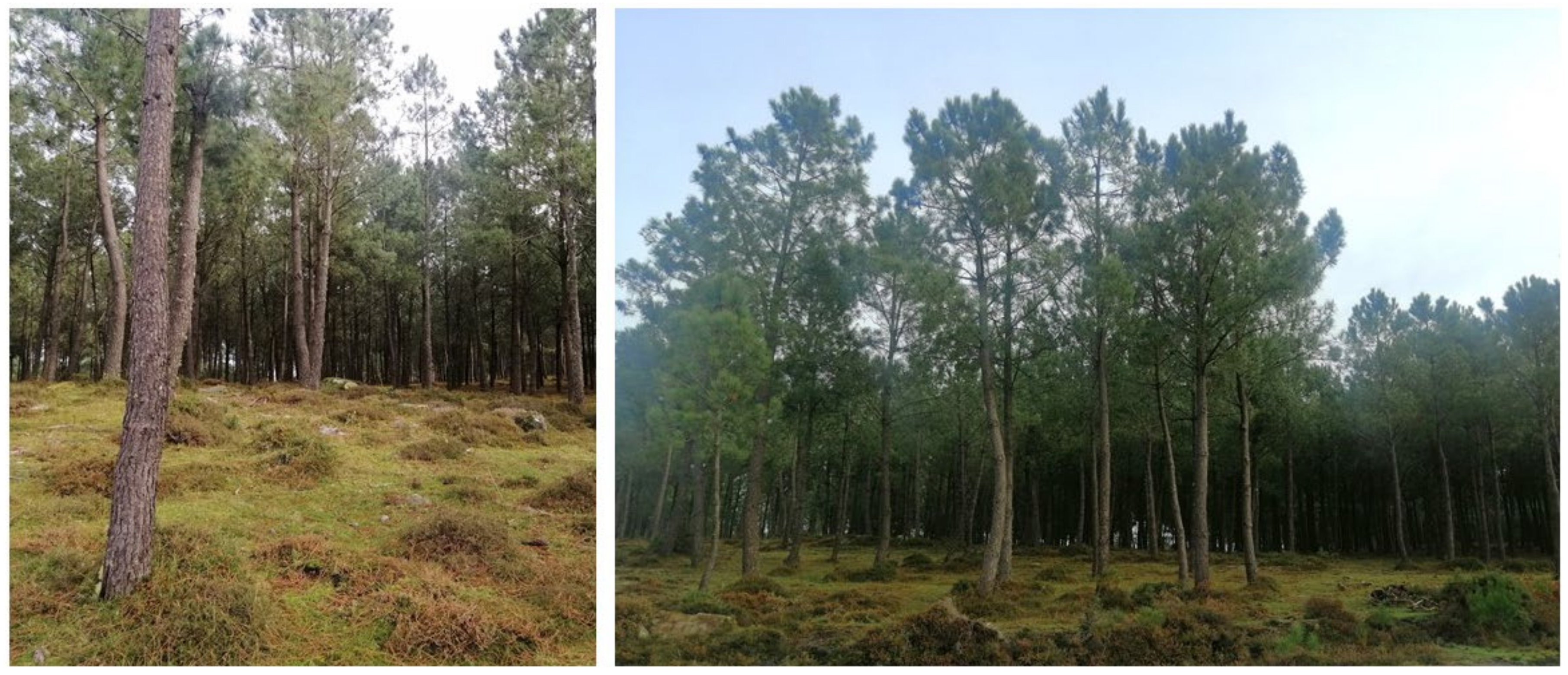
2. Study Area

The study area is in Galicia, a region in the Northwest of Spain (see Figure 1). Galicia is characterized by an active forest sector, with one of the highest harvesting rates in Spain [49,50]. The most common productive species are conifers and Eucalyptus, Pinus pinaster Ait., and Pinus radiata D.Don are the most common species of conifers in the region, according to the latest edition of the Spanish Forest Map [51].

The study was performed in two adjacent stands. The species were identified in situ. Stand 1 is a Pinus pinaster Ait. stand; this plot has a regular planting frame, and pruning has been applied to the individuals. In this stand, there is no understory under the canopy. Stand 2 is a Pinus radiata D.Don stand; it does not have such a regular frame, and the understory is composed of Ulex europaeus L. bushes and Pteridium aquilinum (L.) Kuhn. The average height of stand 1 is 14.10 m, and the average height of stand 2 is 15.6 m; the mean diameter of the stands is 0.31 m for stand 1 and 0.47 m for stand 2; thus, both can be considered high forest systems. The area of the stands is 6064.6 m² and 12,146.4 m², respectively. In stand 1, the mean terrain slope is 8.1% with a standard deviation of 2.6%, and the altitude is between 431.6 m and 439 m. In stand 2, the mean terrain slope is 10.3% with a standard deviation of 5.1%, and the altitude is between 425.2 m and 435.4 m. Figure 2 shows two photographs of stand 1. Figure 3 shows two photographs of stand 2.

3. Materials

The point cloud acquisition was performed with a GeoSLAM^TM ZEB Horizon (GeoSLAM Ltd., Nottingham, UK) [52] scanner. Figure 4 shows an image of the device. This PLS system integrates a scanning head that emits and receives laser pulses in a two-dimensional plane. It is rotatory and uses a time-of-flight principle to estimate the polar coordinates of points that the laser pulse hits. This piece is coupled with a portable platform that contains a motor drive and an inertial measurement unit (IMU). The system uses a novel simultaneous localization and mapping (SLAM) algorithm that combines the two-dimensional laser scanner data with the IMU data to generate three-dimensional point clouds. The scanning head weighs 1.49 kg. The dimensions and weight of the scanner allow the user to carry it easily while walking through the area of interest, capturing the data. A data logger complements the system and registers the data; it also contains the battery for energy supply. This part of the system weighs 1.27 kg. The laser scanner captures 300,000 points per second, providing very high-density point clouds. It has a measurement range of 100 m, an accuracy range that oscillates between 1 and 3 cm, a 270° horizontal field of view, and a 360° vertical field of view.

A GNSS Geomax Zenith15 (GeoMax AG, Wildnau, Switzerland) receiver was used to georeference the obtained point clouds. This system can simultaneously track a maximum of 60 satellites from the GPS, GLONASS, and SBAS constellations. It stands out due to its submeter accuracy and its light weight and portability. It has a height of 95 mm, a diameter of 198 mm, and a weight of 1.2 kg. These characteristics make it optimal for use together with GeoSLAM. The measurement accuracies that can be obtained with this receiver are: static 5 mm + 0.5 ppm (H) and 10 mm + 0.5 ppm (V); static long 3 mm + 0.4 ppm (H) and 3.5 mm + 0.4 ppm (V); kinematic 10 mm + 1 ppm (H) and 20 mm + 1 ppm (V).

Finally, to obtain the altimetry information of the study areas necessary for further processing of the acquired point clouds, the digital terrain model (DTM) was downloaded. There is open access to this model, and it can be downloaded free of charge from the Spanish Geographical Information System (IGN) [53]. This product was developed within the PNOA-LiDAR project (National Plan of Aerial Ortophotography) from aerial LiDAR data captured in 2016 with a density of 1.2 points/m² and a vertical RMSE Z ≤ 25 cm [53,54]. The downloaded DTM (EPSG:25829) has a resolution of 2 m.

For the subsequent processing of the data, the following software was used: GeoSLAM Hub version 6.2.1. [55], LAStools version 211112 [56], R version 4.1.1. [57,58], Python version 3.9. [59], QGIS version 3.8. [60], and FugroViewer version 3.6. [61].

4. Methods

The methodology is divided into 5 subsections. Automatic tree identification and automatic tree segmentation sections are presented separately since it was intended to evaluate the performance of the algorithms for each of these tasks individually.

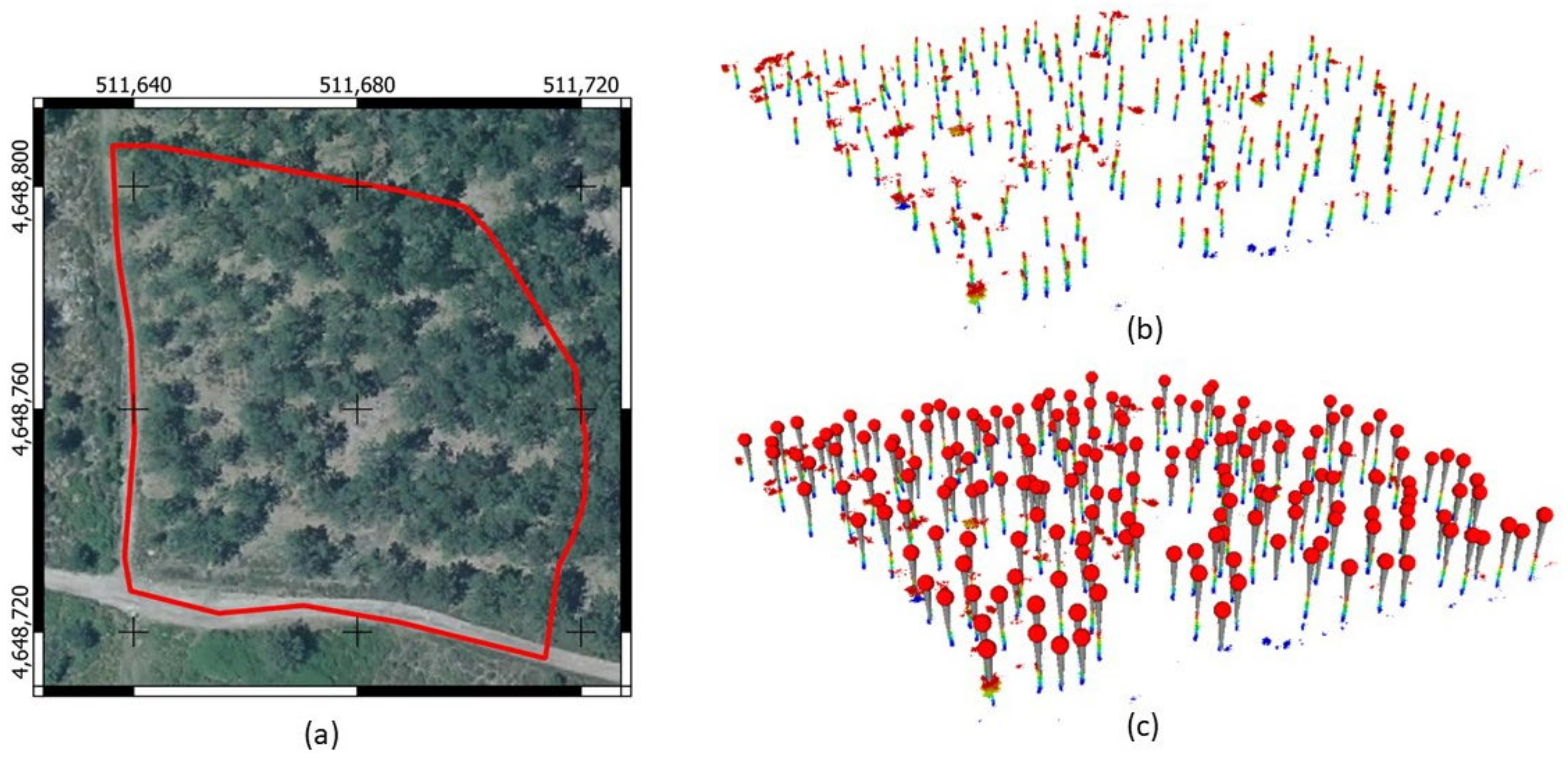
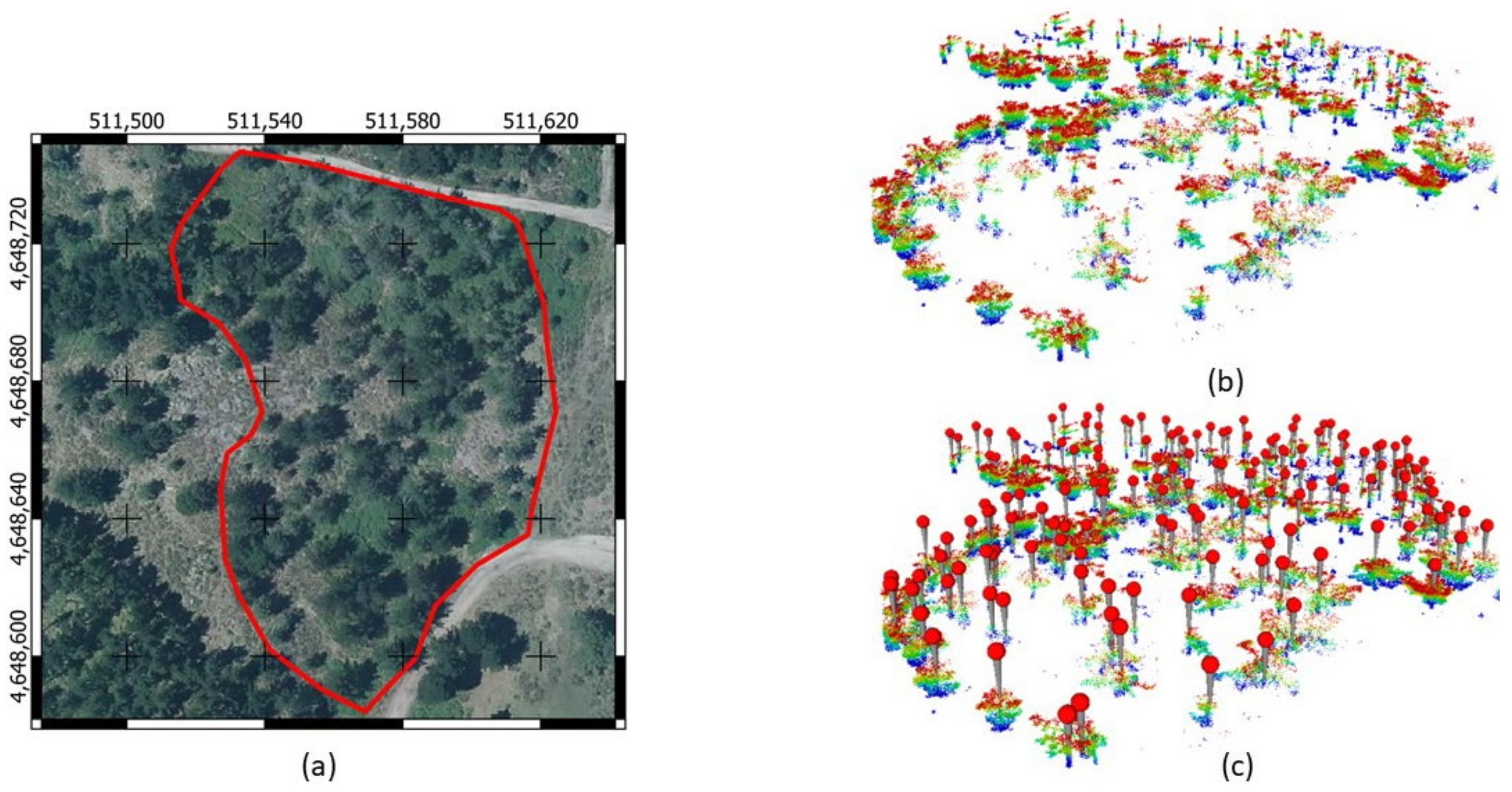
• Point cloud acquisition and georeferencing: Both stands were scanned, and the cartographic coordinates of ground control points were measured to georeference the resulting point clouds;
• Processing of point clouds: The point clouds were processed through normalization, filtering, and rasterization to obtain a canopy height model;
• Ground truth dataset: The real trees were identified and geolocated through visual interpretation of the point clouds;
• Automatic tree identification: Six different identification methods were performed and verified in each stand; three were raster-based methods, and the other three were point-cloud-based methods;
• Automatic tree segmentation: Seven segmentation methods were performed and verified in each stand. Five were raster-based methods, and two were point-cloud-based methods.
• A flowchart of the methodology can be observed in Figure 5.

Figure 5. Flowchart of the general methodology.

Figure 5. Flowchart of the general methodology.

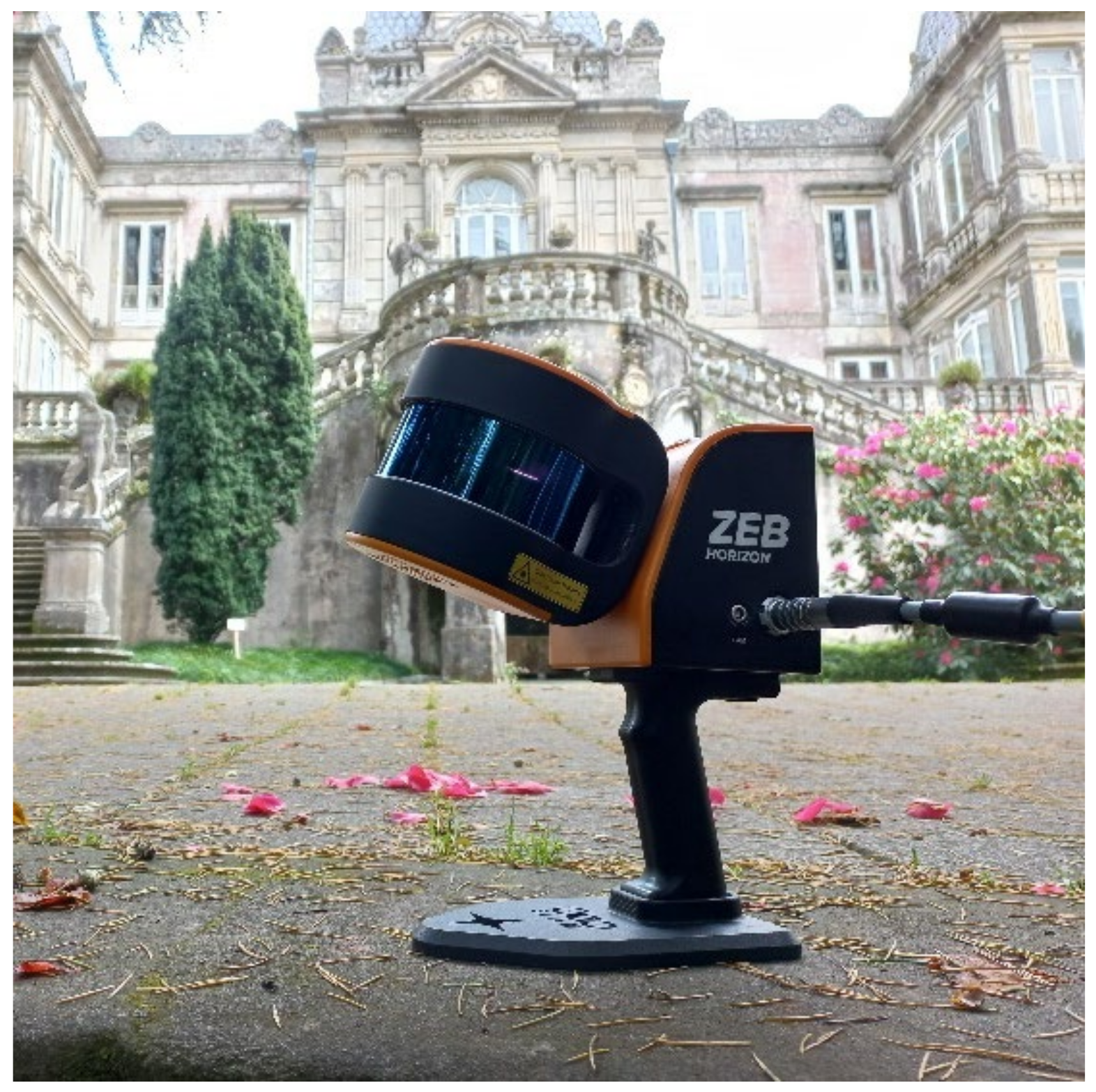
4.1. Point Cloud Acquisition and Georeferencing

Point cloud acquisition using the PLS was executed through independent trajectories, one for each stand. Both were designed as closed paths in order to minimize the SLAM drift [20]. The scanning trajectories were designed to minimize tree occlusions and optimize acquisition time and data size. The raw point cloud from each scanned stand was downloaded from the PLS data logger and pre-processed with GeoSLAM-Hub software version 6.2.1. to yield two independent point clouds, one for each stand.

Table 1. Parameters of raw point clouds.

	Scanning Time (min)	Number of Points (in Millions)	Point Density (pts/m2)
Stand 1	12	90.26	1206.5
Stand 2	17	127.75	1407.47

summarizes the characteristics of these raw point clouds.

A total of 7 ground control points (GCPs) were distributed in a non-linear manner along the acquisition trajectories and outside the canopy cover in order to avoid problems related to the lack of high-quality GNSS under forest cover. Their cartographical coordinates, X, Y, and Z, were measured with the Zenith15 receiver. The point clouds were georeferenced using the GeoSLAM-Hub software. The georeferencing was performed using 4 GCPs for stand 1 and 5 GCPs for stand 2 (2 of the points were in common between the two trajectories).

4.2. Processing of Point Clouds

The processing of point clouds involved normalization and rasterization processes. The normalization process consisted of replacing the orthometric altitude values of the Z coordinates with their height-above-ground values. In order to estimate these heights, the DTM with 2 m of spatial resolution of the study area was used [53,54]. The normalization process was performed with the “lasheight” tool from the LAStools software software version 211112 [56]. The points with values under −0.2 m and above 40 m were removed from the normalized point clouds. The maximum threshold value was established by considering the maximum heights that the analyzed species could potentially reach in the study area. The minimum threshold was established to remove the outliers with high negative values that were obtained due to possible inconsistencies with the DTM.

Afterward, the normalized point clouds were used to obtain the canopy height model (CHM) raster layer for each stand. The CHM was created with the “lidR” package available from the R software version 4.1.1. The algorithm used for this end was the point-to-raster algorithm “p2r”. This algorithm attributes the height of the highest point to each pixel of the raster. Besides, it performs a tweak by replacing each point with 8 points around the original one, emulating the fact that a LiDAR point is not a point but a more realistic disc [62,63]. As a result of this process, the digital value of each pixel in the output file corresponded to the height of the vegetation at that point in space. The pixel size of the CHM was set at 0.5 m to obtain a spatially detailed model, striking a balance between excessive height detail and height generalization.

4.3. Ground Truth Dataset

To determine the location and total number of individuals in each dataset, single trees were identified manually in the normalized point clouds. For this, points below 1 m and above 5 m were removed. In the resulting four-meter-thick slice, tree trunks were clearly recognizable, even amongst surrounding noise points from branches or shrubs. These slices were visualized in a horizontal projection and three-dimensionally in the FugroViewer software version 3.6. The point-of-interest (POI) marking tool was used to manually mark each identified tree trunk within the point clouds. This step was performed for both stands (see Figure 6 and Figure 7). The sets of marked points were exported to a shapefile layer to facilitate their counting. These sets were then used as ground truth datasets for the tree identification process.

4.4. Automatic Tree Identification

Several different methods of tree identification were evaluated. Three of them were oriented at finding treetops in the CHM and the other three were oriented at finding treetops or tree trunks in the point clouds. The reason for comparing the two types of methods is that, for forest species with a high height of the first branch, the identification of tree trunks might provide more accurate results than the identification of treetops [64]. This is the case of the forest species present in stand 1, Pinus pinaster Ait. Additionally, methods based on apical detection may be less efficient in stands of heterogeneous age due to the coexistence of trees with varying heights. This is the case of the forest species present in stand 2, Pinus radiata D. Don. All six of the evaluated methods were applied to both stands.

4.4.1. Treetop Identification through CHM Segmentation (CS)

This method, henceforth referred to as CS, consisted of estimating the coordinates of treetops through the determination of the centroids of CHM-derived watersheds. The first step consisted of obtaining watersheds directly from the CHM raster layer without using initial seeds. The “watershed” function available from the “lidR” package (version 3.1.4) in R was used [62,63]. This function uses the algorithm developed by Pau et al. [65]. It inverts the CHM pixel values, transforming tree crowns into valleys and separating objects that stand out from the background. Watersheds are indexed according to decreasing depth order: the deepest valleys are indexed with the highest values, and the shallowest valleys are indexed with the lowest values. According to the guides of the different packages that were used, the parameters of the algorithms and functions might be configured. To obtain optimum performance, the selection of the parameters was performed through systematic tests for both point clouds, trying to obtain the configuration that could work better in both clouds to make the process as automatic as possible and the results comparable. In this case, three parameters were configured: (1) the threshold height value below which a pixel cannot be considered a tree (th_tree); in this case, it was established at 2 m; (2) the minimum height difference between the highest point of a tree and the point where it touches a neighboring tree (tol); in this case, it was established at 1 m; (3) the radius of the neighborhood in pixels for the detection of neighboring trees (ext), in this case, it was established at 1 pixel. As a result, a new raster layer was created where each pixel value had an identification number (ID) that corresponded to the valley to which it belonged; each valley was assumed to correspond to a single tree crown.

The resulting watershed raster layer was polygonized into a vector layer where each polygon represented the boundary between the different identified watersheds. The geometrical center of each polygon was obtained using the “Centroids” tool in the QGIS software version 3.8. As a result, a new vector layer was obtained containing the centroid points of the CHM-derived watersheds. They were assumed to be the treetops of the trees in the stands analyzed.

4.4.2. Treetop Identification through Point-Cloud Inversion and CHM Segmentation (PCICS)

This method, which will be referred to from this point forward as IPCCS, consisted of estimating tree-trunk positions using an inverted point cloud as the starting input. The first step was to remove all the points from the normalized point cloud that was below 1.8 m, the purpose being to remove all points corresponding to the ground and shrubs. The Z coordinate of each point was then replaced by its corresponding negative integer value. Thus, the lowest values from the original point cloud, the points representing tree trunks, became the highest values and vice versa. A constant was added to the resulting values to make them positive numbers again; in this case, this constant coefficient was 100. This inverted point cloud was used to obtain a CHM, including its watersheds. The same procedure and parameters from the previous section (Section 4.4.1) were used: the “watershed” function from the “lidR” package in R [62,63,65] was used to obtain a raster layer where each pixel value had an identification number (ID) that corresponded to the tree crown to which it belonged. The raster layer was polygonized, and the geometrical center of each polygon was obtained using the “Centroids” tool from the QGIS software. In this case, the centroids of the crown boundary polygons represented an approximation of the position of the tree trunks in the stands analyzed.

4.4.3. Treetop Identification through CHM Local Maxima (CLM)

This method, deemed CLM, consisted of estimating the coordinates of treetops through the determination of the CHM local maxima. It was performed using the “find_trees” tool, which uses a Local Maximum Filter (LMF) and is available in the “lidR” package (version 3.1.4) in R [62,63]. This function analyzes the digital values of the neighboring pixels of each pixel in the CHM and thus determines the local maxima values. In this case, three parameters can be adjusted: (1) the length or diameter of the detection of the local maxima; in this case, it was set at 4 m; (2) the minimum height of a tree to be considered (hmin); in this case, it was established at 3 m; (3) the shape of the window used to find local maxima (shape); in this case, it was established as circular. The output of this algorithm was a shape layer containing the georeferenced points that corresponded to the stand treetops.

4.4.4. Treetop Identification through Point Cloud Local Maxima (PCLM)

This method, which will be referred to as PCLM, consisted of estimating tree trunk positions using the same procedure as in the previous method but using the normalized point cloud as the starting input rather than the CHM raster layer. For each point in the point cloud, the Z coordinate of the neighboring points was analyzed, and the one with the highest value was selected. The “lmf” function was used for this. To use this function, a window size (ws) parameter was established. In this case, the moving window used to detect the local maxima in meters was set at 4. The output of this process was a shape layer containing the georeferenced points that corresponded to the stand treetops.

4.4.5. Tree Trunk Identification through Circle Fitting (CF)

This method, deemed CF, consisted of estimating the positions of tree trunks by slicing the 3D point cloud and fitting circles to tree trucks in the breast height (BH) slice. The methodology is described in detail in Solares-Canal et al. [35]. The first step is slicing the point cloud to obtain a one-centimeter-thick slice at a height of 1.3 m, the standard BH value. In this slice, areas with numerous close points corresponded to tree trunks, and areas with low point densities were considered to be noise corresponding to shrubs or branches. A cluster analysis of the slice was then performed. Specifically, a density-based cluster algorithm was used to group into cluster points that belonged to each tree trunk; for this, the “dbscan” function available from the “dbscan” package in R was used [66]. Two parameters were configured for the stands analyzed: (1) the maximum Euclidean distance allowed between two points for them to belong to the same cluster (eps); (2) the minimum number of points that a cluster must have. The values selected were 0.30 and 10, respectively, for the stand 1 point cloud. For stand 2, the values were 0.40 and 10, respectively. Noise points were assigned to cluster 0 and were discarded.

Once the clusters were identified in the BH slice, the points of each cluster were fitted to circumferences to approximate the perimeters of the tree trunks. Umbach and Jone’s [67] full least-squares method was used. This method minimizes the sum of the squares of the points-to-circles distances. The X and Y coordinates of the geometrical centers of the circles were obtained and stored in a shapefile. Additionally, in the case of stand 2, the radius of each circle was extracted to filter and remove points in the shapefile that corresponded to diameters greater than 1 m or less than 0.10 m. The resulting points were considered to be the estimated positions of the tree trunks in the stands analyzed.

4.4.6. Tree Trunk Identification through Central Axis Estimation (CAE)

This method, which will be referred to as CAE, consisted of estimating tree trunk positions and axis directions by slicing the three-dimensional point cloud, fitting circles to slices at several levels, and adjusting a vector to define tree-trunk axis direction. First, 16 one-centimeter-thick slices were extracted from the normalized point cloud at intervals of 10 cm and starting at a height of 1.0 m. The last slice was thus obtained at a height of 2.50 m. As in the previous case, areas with numerous close points corresponded to tree trunks, and areas with low point densities were considered to be noise corresponding to shrubs or branches. A cluster analysis was then performed in each slice. Points belonging to the same tree trunk were grouped in clusters using the above-mentioned density-based cluster algorithm. Two parameters were configured: the eps was set at 0.2 m, and the minimum number of points in a cluster was set at 10. Points belonging to the same tree trunk were, in this way, grouped together into a cluster.

Once the clusters were identified in each slice, the points from each cluster were fitted to circumferences to approximate the perimeters of the tree trunks at each height level. Umbach and Jone’s [67] full least-squares method was used. The X, Y, and Z coordinates of the centers of the circumferences were obtained and stored in a shapefile along with the corresponding diameters. Since the higher-level slices had high ratios of noise, a filter was used to remove all circles with diameters smaller than 10 cm and greater than 1 m. The density-based cluster algorithm was then used to find centers that were close to one another in space and to discard others. The eps parameter and the minimum number of points were set specifically for each dataset. In the case of stand 1, the configured values were 0.40 m and 5, respectively, and in the case of stand 2, the configured values were 0.30 m and 5, respectively. Clusters that contained more than the expected 16 points (the number of slices) were discarded.

Once the centers of the trees at different heights were found, a three-dimensional vector representing the points belonging to a single tree was established for each cluster. The resulting three-dimensional vectors represented the central axes of the trees; they were saved as points with X, Y, and Z coordinates and vector directions.

4.5. Automatic Tree Segmentation

Several segmentation methods were evaluated; five of them were raster-based, and two of them were point-cloud-based. Some of the methods use the previously identified trees as seeds. All were tested in both of the stands analyzed.

4.5.1. CHM Segmentation (Methods CS_I and CS_II)

This method consisted of segmenting the CHM. The results of this segmentation coincided with the first step that was performed to identify trees in Section 4.4.1. Both the CHM that was obtained from the normalized point cloud and the CHM that was obtained from the inverted point cloud were used. These methods will be referred to as CS_I and CS_II, respectively. As explained in Section 4.4.1, the CHMs were segmented using the “watershed” function from the “lidR” package R [62,63]. As a result, raster layers were obtained where each pixel was assigned to a watershed; then, they were polygonized into vector layers to generate the boundaries of the polygons. Each polygon was assumed to correspond to a tree crown contour. The polygons were vertically extracted, segmenting the 3D point cloud into subsets of point clouds, each representing an individual tree.

4.5.2. CHM Segmentation through 2D Seeding (Methods CS2D_I, CS2D_II and CS2D_III)

This method also consisted of segmenting the CHM. In this case, the Dalponte and Coomes [41] delineation algorithm was used; it is based on the model developed by Hyypä et al. [28] that was initially proposed for ALS data. It was implemented as a function for the “lidR” package in R [62,63]. This algorithm allows for the introduction of user-defined points as starting points. In this case, three different sets of seeding points were built using three of the tree-identification models from the previous section: (1) CLM, (2) PCLM, and (3) CF. Each set contained the tree ID and its X and Y coordinates. According to the inputs used, the different methods were called: (1) CS2D_I, (2) CS2D_II, and (3) CS2D_III.

Once the seeding points were established, the pixel corresponding to each seeding point in the CHM was identified. These were considered to be the initial crown locations where the tree could grow. The four neighboring pixels were considered to be the primary candidates to belong to that tree crown as long as four conditions were fulfilled. The first condition was that the height of the pixel analyzed must be above a certain threshold; in this case, it was defined as 2 m. The second condition was that the pixel height must be greater than a certain percentage of the tree height; this was defined as 45%. The third condition was that the pixel height must be greater than a percentage of the current mean height; this was established as 55%. The final condition was that the crown diameter must be less than 10 m. If these conditions were fulfilled for a pixel, it was considered to belong to the tree. A new digital value corresponding to the ID of the initial seed was then assigned to that pixel. This process was repeated for each seed. The output of this methodology was a raster layer where the digital values of the pixels corresponded to the tree-crown IDs. The final raster was polygonized into a shapefile so that the polygons were vertically extracted, segmenting the three-dimensional point cloud; each tree could be stored independently if required.

4.5.3. Point Cloud Segmentation through Three-Dimensional Seeding (PCS3D Method)

This method, deemed PCS3D, consisted of directly segmenting the normalized point cloud using three-dimensional coordinates of points as seeds. The “segment_trees” function, available from the “lidR” package in R [62,63]., was used. The input data were the three-dimensional point cloud (in a LAS format), and the “dalponte2016” segmentation algorithm was selected. The coordinates of the treetops identified through PCLM were used as seeding points. As a result, an attribute was assigned to each point in the point cloud that corresponded to the ID of the tree to which it belonged. Each tree could be stored independently if required.

4.5.4. Point Cloud Segmentation through Minimum Distances (PCSMD Method)

This method also consisted of segmenting the normalized point cloud. The trunk centers at different heights above the ground, obtained using the CAE method, were used to provide an approximation of the three-dimensional vector that defined the central axes of the tree trunks. An ID was assigned to each of these vectors. The three-dimensional Euclidean distances between each point in the normalized point cloud and the vectors were then calculated. The ID of the nearest vector was assigned to each point in the point cloud, generating a new attribute that corresponded to the tree to which each point belonged. Each tree could be independently stored if required. The three-dimensional Euclidean distances were calculated using the “numpy” package [68] in Python [59].

4.6. Verification

Verification of the results that were obtained through the different tree identification and segmentation procedures was performed for each of the two stands analyzed. In terms of identification methods, it should be noted that the ground truth datasets containing the real tree positions were derived from the estimated centers of trunks. However, the trunk and apex may not always align in some pine species or in the case of some individuals. Furthermore, the tree point with the maximum height may not correspond to the tree apex. For these reasons, buffer zones were created around the points that were obtained through the identification methods. They were used to discern true and false positives: in the horizontal projection, if a real tree was within the buffer zone of an identified tree, it was considered a true positive; if there was no real tree within the buffer zone of an identified tree, this was considered a false positive. Different metrics were calculated:

• The number of identified trees;
• Precision: the number of true positives divided by the total number of trees identified in the stand;
• Recall: the number of true positives divided by the total number of real trees in the stand;
• F-score: the harmonic mean of the precision and recall, calculated as follows:

$$\mathrm{F}-\mathrm{score} (\%)=\frac{N}{\frac{1}{P}+\frac{1}{R}}$$

(1)

where N is the number of considered elements in the harmonic mean, P is the precision, and R is the recall.

In relation to the tree segmentation methods, even though segmentation was performed over previously identified trees, the crowns may be correctly segmented or not. Consequently, these procedures required their own specific verification. In this case, the resulting crown boundaries were compared to the ground truth datasets. The number of real trees encompassed in each boundary was assessed to distinguish between boundaries that represented one and only one real tree (true positives) and boundaries that did not represent a real individual or that included several individuals (false positives). The quality metrics were as follows:

• The number of segmented trees;
• Precision: the number of true positives divided by the total number of trees segmented in the stand;
• Recall: the number of true positives divided by the total number of real trees in the stand;
• Ratio of false positives: the number of false positives divided by the total number of segmented trees in the stand. This metric is provided in total but also differentiates between segmentations that corresponded to groups of real trees and segmentations that did not correspond to any real tree;
• F-score: the harmonic mean of the precision and recall (see Equation (1)).

5. Results

In this section the results obtained in this work are presented. Section 5.1 and Section 5.2 provide the results of the processing of the point clouds. Afterward, the results obtained using the ITD and the ITS methods are presented in Section 5.3 and Section 5.4, respectively. This division aims to enhance clarity and help to a better understanding of them.

5.1. Point Cloud Acquisition and Georeferencing

Independent point clouds were obtained for the two stands. Figure 8 shows screenshots from each of the normalized point clouds. The RMS Error for the georeferencing process in stand 1 is 0.116 m, and in stand 2 is 0.115 m.

Table 2. Adjustment reference points with error values.

		Target			Actual
Stand	GCP	X	Y	Z	X	Y	Z	Error (m)
1	1	511,631.61	4,648,678.33	427.01	511,631.60	4,648,678.25	427.00	0.08
	2	511,683.14	4,648,723.92	432.43	511,683.20	4,648,723.93	432.34	0.11
	3	511,619.03	4,648,812.97	440.67	511,619.01	4,648,813.11	440.82	0.20
	4	511,641.12	4,648,724.98	431.52	511,641.16	4,648,724.99	431.50	0.03
	1	511,631.61	4,648,678.33	427.01	511,631.60	4,648,678.24	427.00	0.09
2	1	511,631.607	4,648,678.326	427.013	511,631.639	4,648,678.316	426.951	0.070
	5	511,618.875	4,648,632.219	425.184	511,618.854	4,648,632.137	425.144	0.093
	6	511,575.815	4,648,583.022	425.315	511,575.796	4,648,582.892	425.333	0.133
	7	511,564.813	4,648,743.541	432.153	511,564.813	4,648,743.647	432.158	0.106
	4	511,641.122	4,648,724.978	431.521	511,641.111	4,648,725.085	431.665	0.179
	1	511,631.607	4,648,678.326	427.013	511,631.626	4,648,678.336	426.949	0.068

shows the error values of the adjustment reference points.

The normalized point clouds of stand 1 and stand 2 have a density of 10,105.86 points/m² and 7185.03 points/m², respectively. The shapes of different species can be appreciated, as well as the stand structure and the presence of understory.

5.2. Processing and Ground Truth

The CHM raster layers obtained for each point cloud (for stand 1 and stand 2) and the ground truth dataset for each stand is shown in Figure 9. The 98th percentile of the CHM height values was obtained at pixel level; the maximum value was then computed for each of the stands. The results were 15.36 m for stand 1 and 18.15 m for stand 2. Through manual tree identification, 188 individuals were counted in stand 1, and 154 individuals were counted in stand 2.

5.3. Automatic Tree Identification

Table 3. Summary of trees identified in stand 1: IT (identified trees); P (precision); R (recall); and F-score.

Method	IT	P (%)	R (%)	F-Score
CS	127	85.9	58.0	69.2
PCICS	200	93.0	98.9	95.9
CLM	159	96.2	81.4	88.2
PCLM	162	96.9	83.5	89.7
CF	192	97.9	100.0	99.0
CAE	189	98.9	99.5	99.2

and

Table 4. Summary of trees identified in stand 2: IT (identified trees); P (precision); R (recall); and F-score.

Method	IT	P (%)	R (%)	F-Score
CS	141	65.3	59.7	62.4
PCICS	178	56.2	64.9	60.2
CLM	166	72.3	77.9	75.0
PCLM	182	69.2	81.8	75.0
CF	236	51.7	79.2	62.6
CAE	117	100.0	76.0	86.4

show the quality metrics obtained for the different tree identification methods in stands 1 and 2, respectively. For stand 1, all of the methods assessed yielded high values for the metrics considered except for CS, which is especially inefficient at detecting individuals: only 58.0% of the total number of real trees were identified with this method. It is precisely this parameter in which the other methods mainly differed: Recall values were less than 84% in CLM and PCLM, while they were over 98% for the other methods. Figure 10 illustrates examples of the results in stand 1. For stand 2, the quality results of the evaluated methods greatly differed in all of the metrics considered. The best results in terms of F-Score were obtained using the CAE method, with a value of 86.4%. The other methods had F-Scores below 76%. Figure 11 illustrates examples of the results in stand 2.

5.4. Automatic Tree Segmentation

Table 5. Summary of segmented trees in stand 1: ST (segmented trees); P (precision), FP (ratio of false positives over the segmented trees), R (recall), F-score.

Method	ST	P (%)	FP (%)					R(%)	F-Score
			0	2	3	4	Total
CS_I	127	59.8	3.1	26.8	6.3	3.9	40.2	40.4	48.3
CS_II	200	94.0	6.0	0	0	0	6.0	100.0	96.9
CS2D_I	159	77.4	2.5	20.1	0	0	22.6	65.4	70.9
CS2D_II	162	80.2	2.5	16.7	0.6	0	19.8	69.2	74.3
CS2D_III	192	92.7	4.7	2.6	0	0	7.3	94.7	93.7
PCS3D	162	79.0	1.9	18.5	0.6	0	21.0	68.1	73.1
PCSMD	189	98.4	1.1	0.5	0	0	1.6	99.0	98.7

and

Table 6. Summary of segmented trees in stand 2: ST (segmented trees); P (precision); FP (ratio of false positives over the segmented trees); R (recall); F-score.

Method	ST	P (%)	FP (%)							R(%)	F-Score
			0	2	3	4	5	6	Total
CS_I	141	69.5	12.8	14.9	2.1	0	0.7	0	30.5	63.6	66.4
CS_II	178	62.4	28.1	6.7	1.1	1.1	0.6	0	37.6	72.1	66.9
CS2D_I	166	72.3	19.9	6.6	1.2	0	0	0	27.7	77.9	75.0
CS2D_II	182	70.3	24.7	4.4	0.5	0	0	0	29.7	83.1	76.2
CS2D_III	236	49.2	48.3	2.5	0	0	0	0	50.8	75.3	59.5
PCS3D	181	71.3	23.8	4.4	0.6	0	0	0	28.7	83.8	77.0
PCSMD	117	72.6	0	17.9	6.8	1.7	0	0.9	27.4	55.2	62.8

show the quality metrics obtained for the different tree segmentation methods in stands 1 and 2, respectively. For stand 1, the methods that provided the highest F-Score values were CS_II, CS2D_III, and PS3D_II; it is worth highlighting that the first of these is also the simplest one in terms of computational processing time. The CS_I method yielded the worst results in all the metrics analyzed. Figure 12 illustrates examples of the results in stand 1.

For stand 2, the quality results of the evaluated methods highly differed in all the metrics considered. The most balanced values were obtained through the CS2D_I, CS2D_II, and PS3D_I methods: Precision values were between 70.3% and 72.3%, total FP values were between 27.7% and 29.7%, and the Recall values were 77.9%, 83.1%, and 83.8%, respectively. The PS3D_I method provided the best results for P and FP: 78.6% and 21.4%, respectively; however, it is quite inefficient at finding individuals (with a Recall value of only 55.2%). Figure 13 illustrates examples of the results in stand 2.

Additionally, the performance of the different segmentation methods was evaluated through visual inspection of the segmented three-dimensional point clouds. An example is shown in Figure 14. This example shows the resulting three-dimensional point clouds of six real trees that were studied using different segmentation methods. It reveals that the CS_I method yielded four trees and overestimated each of the crown contours. The CS2D_I method yielded five trees, one of which was also the result of an overestimation of crown contour. The other methodologies all yielded six trees with different crown–contour segmentations.

6. Discussion

In this section, the findings of this study for ITD and ITS are commented on in Section 6.1 and Section 6.2 respectively.

6.1. Tree Identification

One of the most remarkable findings of the comparison of individual tree identification methods using very high-density point clouds obtained using PLS is that simple raster-based methods can provide very high accuracy metrics in stands with no understory, shrubs, or low branches. This agrees with the results of previous studies [19,26]. The inefficiency of raster-based methods in identifying single trees due to moderate or null apical dominance in the stand can be overcome by inverting the point cloud and subsequently generating a CHM (PCICS method). In doing so, trunks become clear local maxima and can be efficiently identified, providing excellent results in terms of accuracy and recall. The strategy of inverting the point cloud was also proven useful by Xia et al. [23] for identifying individual trees when using TLS point clouds to overcome the problem of occlusions in the tree crowns. The main difference between their approach and the approach presented in this work is that the PCICS method is a raster-based method, and the Xia et al. [23] method is a point-cloud-based method. In general raster-based method is less computationally demanding process compared to the point-cloud-based methods [26]; therefore, the PCICS method would be easily implementable in forest inventories at medium and/or large scales where a large number of plots are measured. Therefore, further testing of this method in tree stands with different structures and with other tree species with similar characteristics (i.e., broad leaves) might be of great interest.

Conversely, the inversion of the point cloud is inefficient in the presence of dense shrubs, understory, and tree branches at low heights since tree trunks do not stand out from these features. Nevertheless, it should be highlighted that tree trunk detection at multiple levels (as addressed by the CAE method) served to mitigate the noise effects of the understory, shrubs, and branches, resulting in 100% precision in stand 2. Even so, the efficiency of the CAE method was moderate in these conditions since trees surrounded by shrubs and branches, which constrained the completeness of the point cloud around the tree trunks and introduced too much noise for the trunk sections to be clearly detected, were not detected. Analogously, other studies have also indicated the difficulty of identifying trees in stands with large amounts of shrubs and branches or with high tree densities [6,27]. Ye et al. and Hyyppä et al. [69,70] indicate that this problematic might be surpassed by including a growth direction parameter in the algorithm. Nevertheless, when performing 3D surveys of these kinds of stands, occlusions should be minimized, and adequate point densities along the tree trunks should be ensured. Consequently, PLS may be the preferred ground platform since it usually outperforms others, such as TLS, in terms of point-cloud completeness [20,35]. In addition, the scanning path should also be chosen with caution to ensure the complete caption of the tree trunks [71].

It might be mentioned that the position of individual trees to use as ground truth was not possible to be identified in the field using the GNSS system, as it would be ideal due to low GNSS signal. Nevertheless, other similar studies have followed the approach of manual identification of the trees over the point cloud [9,37].

6.2. Tree Segmentation

In relation to the segmentation methods assessed, the results show again that the methods are sensitive to stand structure since the same algorithm yielded quite different accuracy metrics for the two stands (precisions differences of 43.5%). Similarly, Burt et al. (2018) concluded that the complexity of the stand greatly affects the performance of the segmentation methods; their algorithm could segment between 96% and 70% of trees depending on the structure of the stand analyzed.

Another matter to remark is that the results are sensitive to the set of seeding points that are used as input. In stand 1, using trunk positions provided better results than using treetop positions. Nevertheless, trunk positions cannot be used as seeds in stands like stand 2 with a great presence of shrubs and branches that prevent accurate trunk surveying; in this case, it is preferable to use treetops as seeds. Some other previous studies have reported the same performance in broadleaves with moderate or null apical dominance [34,72].

The best quantitative and qualitative performance for individual tree segmentation corresponds to point-cloud-based methods: PCSMD in the absence of shrubs and understory and PCS3D in the presence of these features (F-scores of 98.7% and 77.0%, respectively). The study by Zaforemska et al. [33] also concluded that point-cloud-based algorithms provided the most robust results for performing tree segmentation when using a UAV point cloud (F-Score ranging from 80.2% to 90.0%). However, the quantitative superiority of these methods is slight in comparison with some of the other analyzed raster-based methods. In fact, according to Zaforemska et al. [33], raster-based methods are indeed preferred in coniferous forests with a clear apical dominance. Another difference between the results of the point cloud-based and the raster-based algorithms can be found upon visual inspection: the point-cloud-based segmentation methods generate crown boundaries that slightly overlap; they might be more similar to the real crown boundaries with branch imbrications. Nevertheless, it is clear that in complex conditions, the PCSMD method provides feeble results. It may be that the minimum distance criteria could be complemented with crown-boundary-shape criteria or point-connectivity criteria to avoid the incorrect assignation of shrub points to tree trunk axes. Some algorithms developed for tree segmentation in ALS point clouds, such as those described by Burt et al. [45] or Fu et al. [46], could be further evaluated in very high-density point clouds to determine whether higher accuracy metrics can be obtained in complex stands like stand 2.

7. Conclusions

The results showed that the methods in question, both for identification and segmentation, are sensitive to stand structure. The same algorithms provided different accuracy metrics depending on the structure of the stand analyzed. Methods based on finding trunks are more suitable for tree identification in regular stands with no understory. In particular, the PCICS method, a raster-based method based on point-cloud inversion and watershed analysis, proved especially useful for performing tree identification in stands composed of individuals with a high height of the first branch and no understory (this could be extrapolated to broadleaves). This is especially relevant since raster-based methods are not computationally demanding and could hence be implemented on a larger scale for performing single tree identification in medium-scale or large-scale forest inventories.

Regarding tree identification methods for complex stands (stands with a great presence of understory and shrubs), the CAE method, one of the point-cloud-based methods, might be the more suitable. The key parameter to ensure the success of this method is the completeness of the point cloud along the tree trunk.

The segmentation methods evaluated are highly conditioned by the presence of understory and branches in the stand. In the absence of shrubs and understory, the PCSMD, a point-cloud segmentation using minimum Euclidean distances, was determined to be the most suitable. In the opposite situation, it has been found that the PCS3D, a point-cloud segmentation method that uses three-dimensional seeding, was the most adequate. Although raster-based methods can also be useful if the stands are regular and even moderate results in complex stands; however, they are highly sensitive to the initial set of seeding points used.

The results obtained could help technicians select the algorithms to use in different stand conditions for performing automatic tree identification and segmentation using PLS point clouds. Studies like this one could help to augment the operational usage of PLS in forestry.

References

- Bončina, A.; Simončič, T.; Rosset, C. Assessment of the concept of forest functions in Central European forestry. Environ. Sci. Policy 2019, 99, 123–135. [Google Scholar] [CrossRef]
- Oswalt, S.N.; Smith, W.N.; Miles, P.D.; Pugh, S.A. Forest Resources of the United States, 2017: A Technical Document Supporting the Forest Service RPA Assessment; General Technical Report WO-97; U.S. Department of Agriculture, Forest Service, Washington Office: Washington, DC, USA, 2020; 223p. [Google Scholar] [CrossRef]
- Pace, R.; Masini, E.; Giuliarelli, D.; Biagiola, L.; Tomao, A.; Guidolotti, G.; Agrimi, M.; Portoghesi, L.; De Angelis, P.; Calfapietra, C. Tree measurements in the urban environment: Insights from traditional and digital field instruments to smartphone applications. Arboric. Urban For. AUF 2022, 48, 113–123. [Google Scholar] [CrossRef]
- Alonso, L.; Picos, J.; Armesto, J. Mapping eucalyptus species using worldview 3 and random forest. In Proceedings of the ISPRS—International Archives of the Photogrammetry Remote Sensing and Spatial Information Sciences, XLIII-B3-2022, Nice, France, 6–11 June 2022; pp. 819–825. [Google Scholar] [CrossRef]
- Newnham, G.J.; Armston, J.D.; Calders, K.; Disney, M.I.; Lovell, J.L.; Schaaf, C.B.; Strahler, A.H.; Danson, F.M. Terrestrial laser scanning for plot-scale forest measurement. Curr. For. Rep. 2015, 1, 239–251. [Google Scholar] [CrossRef]
- Xie, Y.; Yang, T.; Wang, X.; Chen, X.; Pang, S.; Hu, J.; Wang, A.; Chen, L.; Shen, Z. Applying a Portable Backpack Lidar to Measure and Locate Trees in a Nature Forest Plot: Accuracy and Error Analyses. Remote Sens. 2022, 14, 1806. [Google Scholar] [CrossRef]
- Piermattei, L.; Karel, W.; Wang, D.; Wieser, M.; Mokroš, M.; Surový, P.; Koreň, M.; Tomaštík, J.; Pfeifer, N.; Hollaus, M. Terrestrial structure from motion photogrammetry for deriving forest inventory data. Remote Sens. 2019, 11, 950. [Google Scholar] [CrossRef]
- Bülbül, R.; Reder, S.; Mund, J.P. Performance test of tree segmentation algorithms for WLS point clouds. In Proceedings of the SilviLaser Conference, Vienna, Austria, 28–30 September 2021. [Google Scholar] [CrossRef]
- Yang, Q.; Su, Y.; Jin, S.; Kelly, M.; Hu, T.; Ma, Q.; Li, Y.; Song, S.; Zhang, J.; Xu, G.; et al. The influence of vegetation characteristics on individual tree segmentation methods with airborne LiDAR data. Remote Sens. 2019, 11, 2880. [Google Scholar] [CrossRef]
- Dalla Corte, A.P.; Rex, F.E.; Almeida, D.R.A.; Sanquetta, C.R.; Silva, C.A.; Moura, M.M.; Wilkinson, B.; Zambrano, A.M.A.; Cunha Neto, E.M.; Veras, H.F.P.; et al. Measuring Individual Tree Diameter and Height Using GatorEye High-Density UAV-Lidar in an Integrated Crop-Livestock-Forest System. Remote Sens. 2020, 12, 863. [Google Scholar] [CrossRef]
- Liang, X.; Kukko, A.; Hyyppä, J.; Lehtomäki, M.; Pyörälä, J.; Yu, X.; Kaartinen, H.; Jaakkola, A.; Wang, Y. In-situ measurements from mobile platforms: An emerging approach to address the old challenges associated with forest inventories. ISPRS J. Photogramm. Remote Sens. 2018, 143, 97–107. [Google Scholar] [CrossRef]
- Thompson, I.D.; Maher, S.C.; Rouillard, D.P.; Fryxell, J.M.; Baker, J.A. Accuracy of forest inventory mapping: Some implications for boreal forest management. For. Ecol. Manag. 2007, 252, 208–221. [Google Scholar] [CrossRef]
- White, J.C.; Coops, N.C.; Wulder, M.A.; Vastaranta, M.; Hilker, T.; Tompalski, P. Remote sensing technologies for enhancing forest inventories: A review. Can. J. Remote Sens. 2016, 42, 619–641. [Google Scholar] [CrossRef]
- Liu, H.; Cao, F.; She, G.; Cao, L. Extrapolation Assessment for Forest Structural Parameters in Planted Forests of Southern China by UAV-LiDAR Samples and Multispectral Satellite Imagery. Remote Sens. 2022, 14, 2677. [Google Scholar] [CrossRef]
- Lechner, A.M.; Foody, G.M.; Boyd, D.S. Applications in remote sensing to forest ecology and management. One Earth 2020, 2, 405–412. [Google Scholar] [CrossRef]
- Shugart, H.H.; Saatchi, S.; Hall, F.G. Importance of structure and its measurement in quantifying function of forest ecosystems. J. Geophys. Res. Biogeosci. 2010, 115, G00E13. [Google Scholar] [CrossRef]
- Choi, I.-H.; Nam, S.-K.; Kim, S.-Y.; Lee, D.-G. Forest Digital Twin Implementation Study for 3D Forest Geospatial Information Service. Korean J. Remote Sens. 2023, 39, 1165–1172. [Google Scholar] [CrossRef]
- Michez, A.; Bauwens, S.; Bonnet, S.; Lejeune, P. Characterization of forests with LiDAR technology. In Land Surface Remote Sensing in Agriculture and Forest; Elsevier: Amsterdam, The Netherlands, 2016; pp. 331–362. [Google Scholar] [CrossRef]
- Zhen, Z.; Quackenbush, L.J.; Zhang, L. Trends in automatic individual tree crown detection and delineation—Evolution of LiDAR data. Remote Sens. 2016, 8, 333. [Google Scholar] [CrossRef]
- Gollob, C.; Ritter, T.; Nothdurft, A. Forest inventory with long range and high-speed personal laser scanning (PLS) and simultaneous localization and mapping (SLAM) technology. Remote Sens. 2020, 12, 1509. [Google Scholar] [CrossRef]
- Donager, J.J.; Sánchez Meador, A.J.; Blackburn, R.C. Adjudicating perspectives on forest structure: How do airborne, terrestrial, and mobile lidar-derived estimates compare? Remote Sens. 2021, 13, 2297. [Google Scholar] [CrossRef]
- Hilker, T.; van Leeuwen, M.; Coops, N.C.; Wulder, M.A.; Newnham, G.J.; Jupp, D.L.; Culvenor, D.S. Comparing canopy metrics derived from terrestrial and airborne laser scanning in a Douglas-fir dominated forest stand. Trees Struct. Funct. 2010, 24, 819–832. [Google Scholar] [CrossRef]
- Xia, S.; Chen, D.; Peethambaran, J.; Wang, P.; Xu, S. Point Cloud Inversion: A Novel Approach for the Localization of Trees in Forests from TLS Data. Remote Sens. 2021, 13, 338. [Google Scholar] [CrossRef]
- Yrttimaa, T.; Junttila, S.; Luoma, V.; Calders, K.; Kankare, V.; Saarinen, N.; Kukko, A.; Holopainen, M.; Hyppä, J.; Vastaranta, M. Capturing seasonal radial growth of boreal trees with terrestrial laser scanning. For. Ecol. Manag. 2023, 529, 120733. [Google Scholar] [CrossRef]
- Chiappini, S.; Pierdicca, R.; Malandra, F.; Tonelli, E.; Malinverni, E.S.; Urbinati, C.; Vitali, A. Comparing Mobile Laser Scanner and manual measurements for dendrometric variables estimation in a black pine (Pinus nigra Arn.) plantation. Comput. Electron. Agric. 2022, 198, 107069. [Google Scholar] [CrossRef]
- Latella, M.; Sola, F.; Camporeale, C. A density-based algorithm for the detection of individual trees from LiDAR data. Remote Sens. 2021, 13, 322. [Google Scholar] [CrossRef]
- Vauhkonen, J.; Ene, L.; Gupta, S.; Heinzel, J.; Holmgren, J.; Pitkänen, J.; Solberg, S.; Wang, Y.; Weinacker, H.; Hauglin, K.M.; et al. Comparative testing of single-tree detection algorithms under different types of forest. Forestry 2012, 85, 27–40. [Google Scholar] [CrossRef]
- Hyyppä, J.; Kelle, O.; Lehikoinen, M.; Inkinen, M. A segmentation-based method to retrieve stem volume estimates from 3-D tree height models produced by laser scanners. IEEE Trans. Geosci. Remote Sens. 2001, 39, 969–975. [Google Scholar] [CrossRef]
- Li, W.; Guo, Q.; Jakubowski, M.K.; Kelly, M. A new method for segmenting individual trees from the lidar point cloud. Photogramm. Eng. Remote Sens. 2012, 78, 75–84. [Google Scholar] [CrossRef]
- Lisiewicz, M.; Kamińska, A.; Kraszewski, B.; Stereńczak, K. Correcting the results of CHM-based individual tree detection algorithms to improve their accuracy and reliability. Remote Sens. 2022, 14, 1822. [Google Scholar] [CrossRef]
- Popescu, S.C.; Wynne, R.H. Seeing the trees in the forest: Using lidar and multispectral data fusion with local filtering and variable window size for estimating tree height. Photogramm. Eng. Remote Sens. 2004, 70, 589–604. [Google Scholar] [CrossRef]
- Liu, L.; Lim, S.; Shen, X.; Yebra, M. A hybrid method for segmenting individual trees from airborne lidar data. Comput. Electron. Agric. 2019, 163, 104871. [Google Scholar] [CrossRef]
- Zaforemska, A.; Xiao, W.; Gaulton, R. Individual tree detection from UAV LiDAR data in a mixed species woodland. Int. Arch. Photogramm. Remote Sens. Spat. Inf. Sci. 2019, 42, 657–663. [Google Scholar] [CrossRef]
- Picos, J.; Bastos, G.; Míguez, D.; Alonso, L.; Armesto, J. Individual tree detection in a Eucalyptus plantation using unmanned aerial vehicle (UAV)-LiDAR. Remote Sens. 2020, 12, 885. [Google Scholar] [CrossRef]
- Solares-Canal, A.; Alonso, L.; Picos, J.; Armesto, J. Automatic tree detection and attribute characterization using portable terrestrial lidar. Trees-Struct. Funct. 2023, 37, 963–979. [Google Scholar] [CrossRef]
- Pu, Y.; Xu, D.; Wang, H.; Li, X.; Xu, X. A New Strategy for Individual Tree Detection and Segmentation from Leaf-on and Leaf-off UAV-LiDAR Point Clouds Based on Automatic Detection of Seed Points. Remote Sens. 2023, 15, 1619. [Google Scholar] [CrossRef]
- Tockner, A.; Gollob, C.; Kraßnitzer, R.; Ritter, T.; Nothdurft, A. Automatic tree crown segmentation using dense forest point clouds from Personal Laser Scanning (PLS). Int. J. Appl. Earth Obs. Geoinf. 2022, 114, 103025. [Google Scholar] [CrossRef]
- Hu, B.; Li, J.; Jing, L.; Judah, A. Improving the efficiency and accuracy of individual tree crown delineation from high-density LiDAR data. Int. J. Appl. Earth Obs. Geoinf. 2014, 26, 145–155. [Google Scholar] [CrossRef]
- Yang, J.; Kang, Z.; Cheng, S.; Yang, Z.; Akwensi, P.H. An individual tree segmentation method based on watershed algorithm and three-dimensional spatial distribution analysis from airborne LiDAR point clouds. IEEE J. Sel. Top. Appl. Earth Obs. Remote Sens. 2020, 13, 1055–1067. [Google Scholar] [CrossRef]
- Jing, L.; Hu, B.; Li, J.; Noland, T. Automated delineation of individual tree crowns from LiDAR data by multi-scale analysis and segmentation. Photogramm. Eng. Remote Sens. 2012, 78, 1275–1284. [Google Scholar] [CrossRef]
- Dalponte, M.; Coomes, D.A. Tree-centric mapping of forest carbon density from airborne laser scanning and hyperspectral data. Methods Ecol. Evol. 2016, 7, 1236–1245. [Google Scholar] [CrossRef] [PubMed]
- Huo, L.; Lindberg, E. Individual tree detection using template matching of multiple rasters derived from multispectral airborne laser scanning data. Int. J. Remote Sens. 2020, 41, 9525–9544. [Google Scholar] [CrossRef]
- Lindberg, E.; Eysn, L.; Hollaus, M.; Holmgren, J.; Pfeifer, N. Delineation of tree crowns and tree species classification from full-waveform airborne laser scanning data using 3-D ellipsoidal clustering. IEEE J. Sel. Top. Appl. Earth Obs. Remote Sens. 2014, 7, 3174–3181. [Google Scholar] [CrossRef]
- Brolly, G.; Király, G.; Lehtomäki, M.; Liang, X. Voxel-based automatic tree detection and parameter retrieval from terrestrial laser scans for plot-wise forest inventory. Remote Sens. 2021, 13, 542. [Google Scholar] [CrossRef]
- Burt, A.; Disney, M.; Calders, K. Extracting individual trees from lidar point clouds using treeseg. Methods Ecol. Evol. 2018, 10, 438–445. [Google Scholar] [CrossRef]
- Fu, H.; Li, H.; Dong, Y.; Xu, F.; Chen, F. Segmenting individual tree from TLS point clouds using improved DBSCAN. Forests 2022, 13, 566. [Google Scholar] [CrossRef]
- Li, Y.; Xie, D.; Wang, Y.; Jin, S.; Zhou, K.; Zhang, Z.; Li, W.; Zhang, W.; Mu, X.; Yan, G. Individual tree segmentation of airborne and UAV LiDAR point clouds based on the watershed and optimized connection center evolution clustering. Ecol. Evol. 2023, 13, e10297. [Google Scholar] [CrossRef]
- Comesaña-Cebral, L.; Martínez-Sánchez, J.; Lorenzo, H.; Arias, P. Individual tree segmentation method based on mobile backpack LiDAR point clouds. Sensors 2021, 21, 6007. [Google Scholar] [CrossRef]
- Levers, C.; Verkerk, P.J.; Müller, D.; Verburg, P.H.; Butsic, V.; Leitão, P.J.; Lindner, M.; Kuemmerle, T. Drivers of forest harvesting intensity patterns in Europe. For. Ecol. Manag. 2014, 315, 160–172. [Google Scholar] [CrossRef]
- MITERD. Anuario de Estadística Forestal; Ministerio para la Transición Ecológica y el Reto Demográfico: Madrid, Spain, 2018; Available online: https://www.miteco.gob.es/es/biodiversidad/estadisticas/forestal_anuario_2018.html (accessed on 22 February 2024).
- MITECO. Mapa Forestal de España (MFE) de Máxima Actualidad; Ministerio para la Transición Ecológica y el Reto Demográfico: Madrid, Spain, 2011; Available online: https://www.miteco.gob.es/es/cartografia-y-sig/ide/descargas/biodiversidad/mfe.aspx (accessed on 22 February 2024).
- GeoSLAM-ZEB Horizon. Available online: https://geoslam.com/solutions/zeb-horizon/ (accessed on 22 February 2024).
- Centro de Descargas. Organismo Autónomo Centro Nacional de Información Geográfica. Centro Nacional de Información Geográfica. IGN and MTMAU (Ministerio de Transporte Movilidad y Agenda Urbana and Instituto geográfico Nacional). Available online: http://centrodedescargas.cnig.es/CentroDescargas/index.jsp (accessed on 26 June 2024).
- Especificaciones Técnicas Vuelos PNOA-LiDAR. Available online: https://pnoa.ign.es/pnoa-lidar/especificaciones-tecnicas (accessed on 21 June 2024).
- GeoSLAM Hub 6.2.1. Available online: https://geoslam.com/hub/ (accessed on 22 February 2024).
- Rapidlasso GmbH “LAStools—Efficient LiDAR Processing Software” (Academic). Available online: http://rapidlasso.com/LAStools (accessed on 22 February 2024).
- R Core Team. R: A Language and Environment for Statistical Computing; R Foundation for Statistical Computing: Vienna, Austria, 2013; Available online: http://www.R-project.org/ (accessed on 22 February 2024).
- RStudio Team. RStudio: Integrated Development Environment for R; RStudio, PBC: Boston, MA, USA, 2021; Available online: http://www.rstudio.com/ (accessed on 22 February 2024).
- Python Software Foundation. Python Language Reference, Version 3.9; Python Software Foundation: Wilmington, DE, USA, 2020. [Google Scholar]
- QGIS Development Team. QGIS Geographic Information System. Open Source Geospatial Foundation Project. 2021. Available online: http://qgis.osgeo.org (accessed on 22 February 2024).
- Fugro. Fugro-Fugroviewer. 2021. Available online: https://www.fugro.com/about-fugro/our-expertise/technology/fugroviewer (accessed on 22 February 2024).
- Roussel, J.R.; Auty, D.; Coops, N.C.; Tompalski, P.; Goodbody, T.R.H.; Sánchez Meador, A.; Bourdon, J.F.; De Boissieu, F.; Achim, A. lidR: An R package for analysis of Airborne Laser Scanning (ALS) data. Remote Sens. Environ. 2020, 251, 112061. [Google Scholar] [CrossRef]
- Roussel, J.R.; Auty, D. Airborne LiDAR Data Manipulation and Visualization for Forestry Applications. R Package Version 3.1.4. 2021. Available online: https://cran.r-project.org/package=lidR (accessed on 22 February 2024).
- Valledor, L.; Guerrero, S.; García-Campa, L.; Meijón, M. Proteometabolomic characterization of apical bud maturation in Pinus pinaster. Tree Physiol. 2021, 41, 508–521. [Google Scholar] [CrossRef]
- Pau, G.; Fuchs, F.; Sklyar, O.; Boutros, M.; Huber, W. EBImage—An R package for image processing with applications to cellular phenotypes. Bioinformatics 2010, 26, 979–981. [Google Scholar] [CrossRef] [PubMed]
- Hahsler, M.; Piekenbrock, M.; Doran, D. dbscan: Fast Density-Based Clustering with R. J. Stat. Softw. 2019, 91, 1–30. [Google Scholar] [CrossRef]
- Umbach, D.; Jones, K.N. A few methods for fitting circles to data. IEEE Trans. Instrum. Meas. 2003, 52, 1881–1885. [Google Scholar] [CrossRef]
- Harris, C.R.; Millman, K.J.; Van Der Walt, S.J.; Gommers, R.; Virtanen, P.; Cournapeau, D.; Wieser, E.; Taylor, J.; Berg, S.; Smith, N.J.; et al. Array programming with NumPy. Nature 2020, 585, 357–362. [Google Scholar] [CrossRef] [PubMed]
- Ye, W.; Qian, C.; Tang, J.; Liu, H.; Fan, X.; Liang, X.; Zhang, H. Improved 3D stem mapping method and elliptic hypothesis-based DBH estimation from terrestrial laser scanning data. Remote Sens. 2020, 12, 352. [Google Scholar] [CrossRef]
- Hyyppä, E.; Kukko, A.; Kaijaluoto, R.; White, J.C.; Wulder, M.A.; Pyörälä, J.; Liang, X.; Yu, X.; Wang, Y.; Kaartinen, H.; et al. Accurate derivation of stem curve and volume using backpack mobile laser scanning. ISPRS J. Photogramm. Remote Sens. 2020, 161, 246–262. [Google Scholar] [CrossRef]
- Tupinambá-Simões, F.; Pascual, A.; Guerra-Hernández, J.; Ordóñez, C.; de Conto, T.; Bravo, F. Assessing the performance of a handheld laser scanning system for individual tree mapping—A Mixed forests showcase in Spain. Remote Sens. 2023, 15, 1169. [Google Scholar] [CrossRef]
- Lu, X.; Guo, Q.; Li, W.; Flanagan, J. A bottom-up approach to segment individual deciduous trees using leaf-off lidar point cloud data. ISPRS J. Photogramm. Remote Sens. 2014, 94, 1–12. [Google Scholar] [CrossRef]