Article

The Application of Percolation Theory in Modeling the Vertical Distribution of Soil Organic Carbon in the Changbai Mountains

College of Forestry, Beihua University, Jilin City 132013, China
*
Author to whom correspondence should be addressed.
Forests 2024, 15(7), 1155; https://doi.org/10.3390/f15071155
Submission received: 29 May 2024 / Revised: 29 June 2024 / Accepted: 2 July 2024 / Published: 3 July 2024
(This article belongs to the Special Issue Forest Soil Carbon and Climate Change)

Abstract

:
A power-law formulation rooted in percolation theory has proven effective in depicting the vertical distribution of soil organic carbon (SOC) in temperate forest subsoils. While the model suggests the solute as the primary factor distributing SOC, this may not hold true in the surface soil in which roots contribute significantly to the SOC. This study in the Changbai Mountains Mixed Forests ecoregion (CMMF) evaluates the SOC profiles in three forests to assess the model’s efficacy throughout the soil column. Prediction of the SOC profile based on the regional average values was also assessed using field data. The observed scaling aligned well with predictions in mixed broadleaved and broadleaved Korean pine mixed forests, but disparities emerged in birch forest, possibly due to waterlogging. The predicted SOC levels correlate strongly with the field data and align well with the normalized average SOC levels. The findings suggest that the model remains applicable in the CMMF when considering root-derived carbon. However, the hindrance of solute transport may have a greater impact than roots do. The spatial heterogeneity of the SOC means that a single predicted SOC value at a specific depth may not fit all sites, but the overall agreement highlights the potential of the model for predicting the average or representative SOC profiles, which could further aid in regional-scale carbon stock estimation.

1. Introduction

Temperate forests play an essential role in the global carbon cycle, representing 34% of the total carbon sink in established forests worldwide [1]. As soil serves as the largest reservoir of organic carbon in terrestrial ecosystems, understanding the dynamics and quantity of soil organic carbon (SOC) in temperate forests is crucial for research on mitigating global warming. While the spatial distribution of the SOC has been studied and mapped using various methods such as GIS and remote sensing techniques (e.g., [2,3,4,5]), the models developed are typically two-dimensional and focus mainly on the surface layer of soil. Nevertheless, the soil profiles have indicated a substantial quantity of SOC stored below the surface layer of soil [6]. Therefore, including deeper soil layers in the SOC predictions is essential for enhancing SOC stock estimation in forest soils. In contrast to the extensive studies on the spatial variability in the SOC, research on the vertical patterns and the dynamics of SOC remains relatively limited [7]. Typically, the SOC concentration decreases with soil depth, with the majority of SOC retained in the topsoil. The vertical distribution of SOC in forest soils is shaped by the long-term accumulation of carbon in the soil, originating predominantly from both above- and belowground biomass [8,9]. The dramatic decrease in SOC content with depth may be attributed to the distinct major sources of carbon in the surface and subsurface soil. Carbon derived from above-ground biomass, such as plant debris and leaf litter, tends to accumulate in the topsoil (~10 cm) [8,10]. This accumulation is heavily influenced by climate, vegetation, and soil texture, contributing to the spatial variability in SOC levels [11]. In contrast, below the topsoil, carbon input from the aboveground litter is limited [8,10,12,13], whereas carbon derived from roots and downward transport from the upper layers can act as substantial carbon sources [14,15,16]. Meanwhile, the SOC from the displacement and deformation of the soil matrix can be extremely slow [17]. Therefore, the SOC level at a given soil depth is influenced by multiple factors, such as carbon turnover in aboveground biomass, root turnover and distribution, and solute transport delivering carbon into deeper soil layers, all of which can be affected by climate and vegetation cover. Among these factors, carbon added from roots and carbon conveyed by solute transport can significantly impact the vertical pattern of the SOC, as both are the major carbon sources in deep soils and can extend to a considerable depth in the soil column. Various mathematical functions have been proposed to describe the decline of SOC with depth, including the log–log model (e.g., [11,18]), polynomial and exponential-based functions (e.g., [6,19]), and the power-law model (e.g., [20,21,22,23]). Within these, exponential functions and power-law functions are the most frequently employed. Both exponential and power-law functions are commonly employed to illustrate non-linear trends in various ecological systems, with power-law functions particularly utilized to describe fractal-like behaviors. While these functions effectively capture the non-linear characteristics of SOC depth profiles, their interpretability regarding ecological processes is often limited in many applications [24]. Moreover, parameters in most functions that quantify the relative decline of SOC with depth typically vary across sites, even within the same biome. However, a specific power-law function has been proven to effectively describe the decline of SOC with soil depth in the tropical and subtropical regions of China with a fixed rate of −1, expressed as follows: C = 1 / ( a + b h ) , where C represents the SOC content (%), h denotes soil depth (cm), and a and b are two adjustable parameters [20]. This power-law relationship describes the correlation between SOC levels and depth, with the relationship of h     C 1 , yet it also lacks clarity regarding the ecological relevance of these parameters. In a recent study focused on temperate forests, Yu et al. [23] presented a similar power-law model derived from percolation theory, represented as t     h D b , where t is the solute transport time in soil, and Db is the fractal dimensionality of the percolation backbone, a well-established value determined by the dimensionality and saturated condition of the percolating medium [25]. The percolation model was developed under the assumption that the water percolating downward in the sublayer of soil is the key factor that redistributes the SOC [23]. This results in the vertical distribution of the SOC being influenced by the vertical solute transport, where the solute transport time scales with the transport distance as t     h D b . In the context of temperate forest soils, a 3D saturated condition of the flow was considered, with Db = 1.87 as referenced by Sheppard et al. [26]. Consequently, the rate of SOC delivery can be calculated by finding the time derivative of soil depth, yielding R s o c h 0.87 . This percolation model distinguishes itself from other existing power-law models by providing a well-defined Db value that characterizes the decline in SOC levels with soil depth, solely determined by the dimensionality and saturation of the percolating medium and independent of other soil properties. This achievement stems from employing critical path analysis within its theoretical framework, which quantifies all distinct solute transport paths connectable through the system and their associated fluid fluxes [25]. Knowing the topology of each path system and their associated fluid fluxes allows for calculating the total solute transport time, and the scaling relationship between the solute transport time and the transport distance is observed to be governed by the fractal dimensionality of the percolation backbone Db. With the hypothesis that the SOC from the topsoil is the primary source of carbon in the subsoil, the vertical scaling of the SOC concentration, Csoc, with the soil depth can be described as follows [23]:
C s o c h 0.87     o r       h C s o c 1.149 ,
Equation (1) can be reformulated into a more practical format to predict the SOC at any given depth, h,
C S O C ( h ) = ( h h s ) 0.87 ×   C s
Cs is a known SOC concentration value at soil depth hs at a specific site; it is important to note that Cs may vary across sites at the same soil depth hs, due to the spatial variability in the SOC.
Equation (1) exhibits proximity in the exponent value to the established power-law function of −1 as described in Li and Zhao [20], with an exponent of −1.149, specifically relevant to the solute transport processes. The percolation model has effectively depicted the vertical scaling of the SOC in temperate forest soils across various scales, yet its application has been limited to subsoil layers below 20 cm in which the majority of the root biomass in temperate forests is concentrated [23]. This limitation arises because the model assumes that the primary source of SOC is from the downward movement of solutes, neglecting the carbon input from other sources. This assumption may not hold true in the top layer of soil as carbon emerges from multiple sources both above and below ground, including plant debris, leaf and root litter, and SOC transported from the soil above [8,9,15]. The addition of carbon to the SOC from sources besides solute transport, particularly from fine roots, can significantly impact SOC redistribution, potentially causing a vertical pattern of SOC distribution that is different from the one that is described by percolation theory. Therefore, whether Equation (1) is adequate for describing the vertical distribution of SOC across the entire soil column, accounting for both the topsoil and subsoil, hinges on the extent of the influence exerted by the vertical distribution of additional carbon from roots.
In this study, we utilized Equation (1) to simulate the vertical pattern of SOC in the Changbai Mountains Mixed Forests ecoregion to evaluate the validity of the model in describing the vertical distribution of the SOC while considering the entire soil column. This study sought to investigate the impact of roots on the adequacy of the percolation mode, thereby enhancing the understanding of both the applicability and limitations of the model within the region. The Changbai Mountains Mixed Forests ecoregion (CMMF, 41°45′ N, 127°45′ E) spans over 93,000 km2, encompassing the Changbai Mountains and surrounding foothills across China and North Korea. This vast region features a diverse landscape with an extensive coverage of mixed coniferous and broadleaf trees, alongside subalpine vegetation. Known for its richness, the CMMF serves as a vital component of the northeast forest ecosystem in China, supporting a wide array of flora and fauna within its expansive boundaries and significantly influencing the carbon budget in mid- to high-altitude forest ecosystems [27]. A comprehensive understanding of the vertical distribution of SOC and the applicability of the percolation model will contribute to advancing methodologies in carbon cycling prediction and improving the accuracy of forest SOC inventories within this geographical domain. Moreover, its varied forest typologies provide valuable comparative insights for temperate forest ecosystems. The CMMF area includes various forest types, such as deciduous, mixed conifer–broadleaved, coniferous, and birch forests. Soil profiles were sampled from three typical forest types: mixed broadleaved forest, birch forest, and broadleaved Korean pine mixed forest, to examine the validity of Equation (1). A predicted model utilizing Equation (2) with an adjustable parameter Cs along with its corresponding depth hs, as determined by historical sampling data, was also established to predict the vertical distribution of SOC within the CMMF. Given the spatial variability in the SOC, it is anticipated that SOC values observed at different sites will vary at the same depth. While Equation (2) yields a single predicted SOC value at a specific soil depth, it is essential to recognize that this value represents an average or representative estimate derived from the model.

2. Materials and Methods

2.1. Study Site and Field Sampling

The study presented comprised two distinct sampling events. To examine the effect of roots on the efficacy of Equation (1) in describing the vertical distribution of SOC in the CMMF, soil profile specimens were gathered from Jingyu, China, constituting a segment of the broader Changbai Mountain forest ecosystem. Due to the vast expanse of the region, sampling based on forest types is commonly effective in ensuring the representativeness of soil samples. Therefore, three typical forest types within the CMMF were selected as sampling sites: a birch forest (Betula platyphylla, BF), a mixed broadleaved forest (MBF), and a broadleaved Korean pine mixed forest (BKF) (site details are displayed in Table 1). The region exhibits a temperate monsoon climate with an average annual precipitation of 767 mm and an average annual temperature of 3.7 °C. The principal tree species encompass Betula platyphylla, Ulmus davidiana Planch, and Maackia amurensis within the BF; Fraxinus mandshurica, Betula platyphylla, and Ulmus davidiana Planch within the MBF; and Pinus koraiensis, Populus ussuriensis, and Acer mono within the BKF. The soils present at all three sites are classified as humic Cambisols, with distinct manifestations of gleyic characteristics at depths ranging from 0.3 to 0.4 m within the BF, attributable to seasonal waterlogging. Three 20 m × 30 m plots were established within each forest area, with five sampling points randomly designated within each plot. Given that the C layers of soil were shallower than 0.6 m in all sampling plots, soil samples were extracted using a stainless-steel corer down to a depth of 0.7 m and were subsequently subdivided into 7 soil samples, with a depth increment of 0.1 m for further SOC analysis.
The vertical distribution of the SOC could be predicted utilizing Equation (2) with the provided values of Cs and hs specific to a particular site. Extended to a broader region such as the CMMF, a regionally averaged Cs at its corresponding depth hs could aid in predicting the most probable vertical distribution of the SOC. Therefore, the accuracy of the prediction greatly depends on the accuracy of the Cs and hs estimation for the region. Given the diverse nature of forest ecosystems in the region, spatial variability in the SOC is anticipated. A larger dataset covering a broader spectrum of forest types within the region would enhance the estimation. Therefore, to acquire the most representative estimates of Cs and hs, historical SOC data from 43 plots covering all the major forest types in the region (details shown in Table 2) from our previous sampling events for a different research objective were utilized to determine the parameters Cs and hs in Equation (2). The soil profiles were sampled with a consistent methodology, with the deepest sampling depth reaching 0.5 m. Subsequently, the sampled soil profiles were further divided into 4 soil samples, spanning 0–0.1 m, 0.1–0.2 m, 0.2–0.3 m, and 0.3–0.5 m in depth for SOC analysis. Soil samples from the two sampling events were naturally air-dried with any plant residue removed. Samples belonging to the same soil increment, obtained from the 5 replicates within each plot, were mixed as one sample prior to analysis. Subsequently, the dried samples were subjected to milling and sieving through a 100-mesh screen before undergoing analysis. The SOC concentration (g/kg) within each soil increment was determined using the potassium dichromate oxidation method with external heating.

2.2. Data Analysis

2.2.1. Vertical Distribution of SOC in CMMF

The SOC depth profiles of individual plots in Jingyu were established through plotting the SOC concentration of each soil increment against the midpoint of its corresponding interval. The vertical distribution of the SOC within each forest was represented by averaging the soil profiles obtained from 3 plots within each forest. The SOC depth profiles, both inclusive and exclusive of the upper 20 cm, were subjected to fitting with a power-law function to assess the impact of carbon emerging from roots on the efficacy of Equation (1) in describing the vertical distribution of the SOC across the entirety of the soil profile within the site. The resulting scaling exponents from the power-law function were compared with the theoretical exponent, −1.149, in Equation (1) to examine the degree of concordance between the theoretical scaling and observation. In the BF forest, waterlogging occurs within the depth range of 0.3 to 0.4 m, thereby influencing the vertical transport of solute below this soil depth. Consequently, soil profiles above 0.3 m in the BF were also subjected to fitting with a power-law function, aimed at mitigating the impact of waterlogging on the solute transport dynamics. One-way analysis of variance (ANOVA) was additionally employed to investigate the influence of the forest type on the SOC content across individual soil depth increments.

2.2.2. Prediction of SOC Profile in CMMF

Equation (2) was utilized to predict the most representative vertical distribution of SOC in the CMMF using regionally averaged Cs values at a suitable depth hs, calculated from the SOC profiles obtained from the 43 plots during the previous sampling event. Since the surface soil is more susceptible to external influences and deeper soil at certain locations may experience waterlogging, the average Cs values of the 0.2–0.3 m soil layer (hs = 0.25 m) were chosen for Equation (2) to reduce any errors that may impact the estimation. Subsequently, Equation (2) was evaluated through a comparison between the prediction and the observed SOC soil profiles collected within the region from 14 published studies [19,20,21,22,23,24,25,26,27,28,29,30,31,32] (details are displayed in Table 3). The spatial variability in the SOC levels across different sites from different studies can lead to significant scatter at a given soil depth. This variability poses a challenge when comparing predicted SOC values, which typically provide a single estimate for a given depth. To address this, a data normalization procedure based on the soil depth was also applied to the field data. This procedure aimed to determine the most probable SOC level at a given soil depth for comparison with the model predictions. The data normalization method involves categorizing observed soil profiles based on specific soil depth intervals (0–0.1, 0.1–0.2, 0.2–0.3, 0.3–0.4, 0.4–0.5, 0.5–0.6, 0.6–0.8, 0.8–1.0, in meters). Subsequently, the average SOC value is computed for each group, with the midpoint of each soil depth interval serving as the corresponding depth for that group.

3. Results

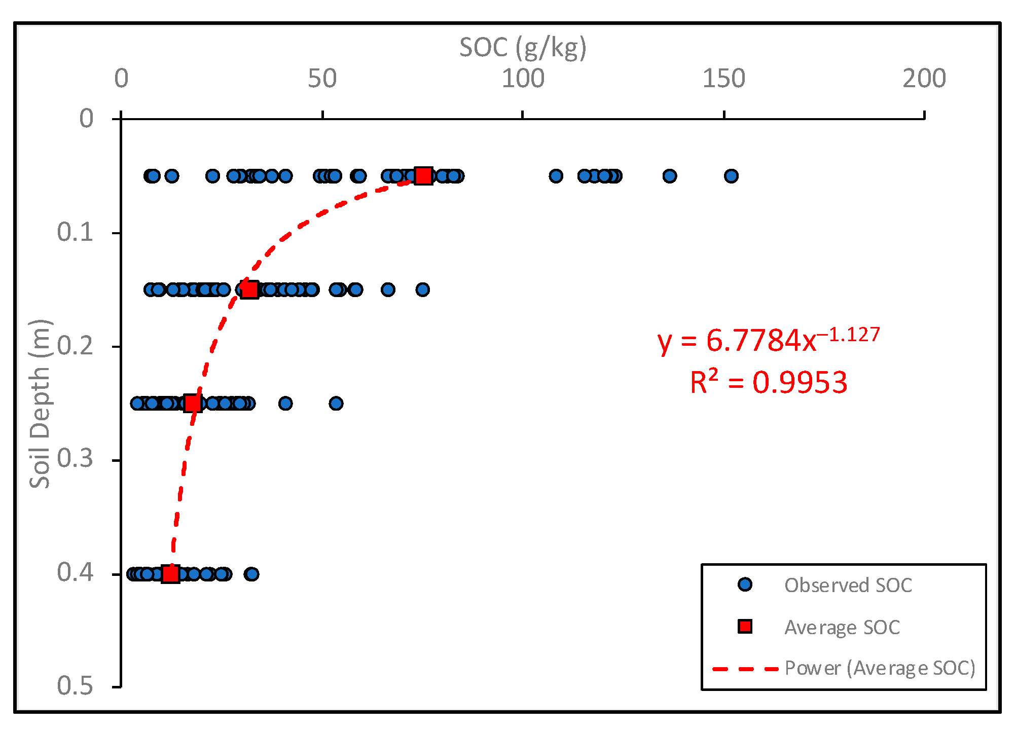
3.1. Vertical Distribution of SOC in Three Forests in CMMF

As depicted in Table 4, the SOC concentration decreased with increasing soil depth across all three forest types. A significant decrease in SOC levels below the 0.4–0.5 m soil layer was observed in the BF forest compared to the other two forests, suggesting that forest type or soil texture may have a greater impact on the SOC concentration in deeper soil layers. The vertical distribution of SOC in all three forest soils can be characterized using a power-law function, as depicted in Figure 1. Comparable scaling exponents were derived for both MBF and BKF soils, with values of approximately −1.077 and −1.086, respectively (see Figure 1a). These values closely align with the theoretical exponent of −1.149. At the BF site, the SOC concentration exhibits a notably rapid decrease, characterized by a power scaling of −0.582. This implies that Equation (1) might not fully capture the vertical distribution of SOC at this specific site, potentially due to the hindrance of SOC downward movement via solute transport below 0.3–0.4 m. This obstruction leads to notable declines in the SOC concentration beyond that depth, likely attributed to waterlogging at the 0.3 to 0.4 m depth. Considering only the top three data points (soil depth from 0 to 0.3 m), the power exponent decreases to −1.156 (“BF-top” in Figure 1a), which closely approximates the theoretical −1.149. This suggests that Equation (1) may still be applicable for describing the vertical pattern of SOC in the soil above 0.3 m at the BF site, indicating a consistent vertical pattern of SOC distribution across the three studied forest soils. Excluding the topsoil (soil above 0.2 m, Figure 1b) to reduce impact from root-derived carbon, comparable exponents were found in the MBF (−1.039 vs. −1.077) and BKF (−1.027 vs. −1.086). In the BF, however, the exponent shifted to −0.361, deviating significantly from the theoretical value of −1.149. This deviation could again be attributed to the inhibition of solute transport due to waterlogging.

3.2. Effect of Forest Type on Vertical Distribution of SOC

The results of the one-way ANOVA conducted on the SOC concentration at identical soil depth across the three forests indicate no significant difference in the SOC concentration at a depth above 0.45 m among the three forest types (Table 4). Although significant differences in the SOC below 0.45 m were observed, there was no significant distinction in the SOC between the MBF and BKF sites. The notable variation in the SOC among the three sites may be attributed to the rapid decrease in the SOC below 0.3–0.4 m due to waterlogging at the BF site. The findings suggest that the influence of forest type on SOC quantity in the three forest types at equivalent soil depths is not significant.

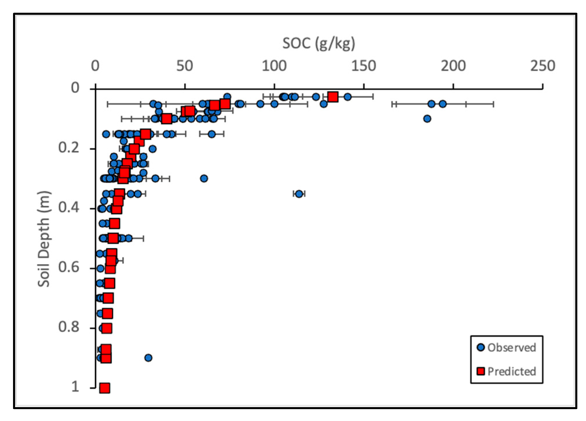
3.3. Prediction of Vertical Distribution of SOC in CMMF

Figure 2 represents the SOC profiles collected from 43 plots during the previous sampling event, along with the average SOC profile. The average SOC content in the 0.2 to 0.3 m soil layer across the 43 plots in the CMMF was 17.874 g/kg. Therefore Cs = 17.874 g/kg and hs = 0.25 m were applied in Equation (2) to predict the vertical distribution of the SOC in the region. In Figure 3 and Figure 4, the SOC concentration predicted using Equation (2) was compared against observed SOC values from 14 published studies (encompassing over 300 soil profiles) in the CMMF. The significant dispersion observed in comparison to the 1:1 line in Figure 4 is likely due to the substantial spatial variability in the SOC at a specific depth across the various studies as shown in Figure 3. This is because Equation (2) provides a single value at a particular depth, whereas the actual data exhibit significant variability. With the intercept set to 0, the linear model fitted to all data points yielded a coefficient of 1.0172. This suggests that the predicted SOC at a given depth using Equation (2) might represent the average or the most probable value of SOC at that depth across sites within the region. This is further supported by comparing the predicted value to the normalized SOC values, where a coefficient of 1.0241 was obtained and all data points closely aligned with the 1:1 line.

4. Discussion

The exponents resulting from the power-law fitting to the SOC depth profiles in the BKF, MBF, and soil above the water-logged soil layer at the BF site were consistent with the theoretical value of −1.149. In contrast to deeper soils in which the root biomass declines sharply and SOC input primarily occurs through downward carbon movement via solute transport, the surface soil layer presents a more intricate scenario due to its diverse carbon sources, encompassing input from both aboveground and belowground biomass. However, the power-law exponents from fitting, whether including or excluding the top 20 cm of soil, align closely with the theoretical value of −1.149 and exhibit no significant difference at both MBF and BKF sites. This implies that Equation (1) remains applicable in delineating the vertical distribution of SOC across the entire soil column at the study sites even when factoring in the influence of other carbon sources in the surface soil. Of these sources, carbon from roots, notably fine roots that serve as a significant carbon source [12,41], has the potential to shape a different vertical SOC pattern than what percolation theory outlines. This is due to the variability in the carbon input from roots along the soil column, influenced by the root turnover and the distribution of the root system in the soil. Therefore, the vertical distribution of SOC is primarily influenced by the combined contribution of carbon supplied by roots and carbon conveyed from the upper layer of soil through solute transport, the latter of which can be effectively described by Equation (1). Consequently, the impact of the roots and the solute transport on the vertical SOC pattern is subjected to factors affecting both the magnitude and the relative importance of the carbon input from these sources, with climate and vegetation type being the potential key determinants exhibiting a significant correlation with the SOC levels in a previous study conducted by Jobbágy and Jackson [11]. However, on a global scale, climate demonstrates a stronger correlation with the total amount of SOC in the first meter, whereas its correlation with the vertical distribution of SOC is less pronounced compared to the strong correlation observed between SOC vertical patterns and vegetation types. Therefore, the influence of climate on the vertical distribution of SOC is limited and potentially overshadowed by the impact from vegetation [11]. The vegetation type determines the vertical distribution of root systems and the allocation of plant biomass above and below ground, thereby significantly influencing the carbon input throughout the soil column. For instance, both a deeper root system and a lower aboveground biomass could enhance the influence from roots on the vertical pattern of the SOC. A deeper root system continuously adds carbon throughout the soil, and a lower aboveground biomass diminishes the carbon input from the upper soil layers through solute transport, thereby amplifying the impact of carbon derived from fine roots. Hence, with an increasing influence from roots, the disparity between the theoretical scaling proposed by Equation (1), which solely accounts for carbon input from solute transport, and the observed SOC profile is likely to expand.
Global reviews of root distribution and plant biomass allocation above and below ground across various biomes reveal that grasslands generally display the shallowest root profiles, while shrublands have the deepest root profiles and forests fall between these two extremes in terms of root depth. Additionally, forests exhibit a significantly higher proportion of biomass aboveground compared to grasslands, while shrublands show intermediate values [11,42]. Therefore, among the three biomes, the influence of roots on the vertical pattern of SOC should be the least in forests and the highest in shrublands. This is further supported by the disparities between the theoretical value of −1.149 and the exponents extracted from the power-law fitting of the SOC profiles of these biomes based on global summarized data [11] by Yu et al. [23], with exponents of −1.105 in forests, −1.347 in grasslands, and −2.127 in shrublands. Although the global-scale vertical distribution of SOC in forests aligns with the percolation model, discrepancies may arise when focusing on specific forest types. Table 5 presents a summary of the power-law exponents for the vertical distribution of SOC, as well as the proportions of aboveground biomass, the index of rooting distribution of fine roots (higher β values imply deeper rooting profiles), and the proportion of fine roots biomass above 30 cm across various types of forests [11,43]. The exponents reveal that the vertical distribution of SOC in temperate deciduous and evergreen forests closely aligns with the theoretical scaling, whereas there is greater disparity in tropical and boreal forests. This is likely due to variations in both forest type and environmental conditions that can impact soil hydrological processes or the transport of SOC in the soil.
Temperate forests, such as the CMMF studied here, differ from boreal and tropical forests due to their moderate climate, which results in fewer disturbances to soil hydrological processes such as soil frost, waterlogging, and significant soil leaching by intensive rainfall. Moreover, temperate forests have a high proportion of aboveground biomass and relatively shallow fine root systems compared to other forests, which minimizes the influence of root-derived carbon on the vertical distribution of SOC. In tropical evergreen forests, despite the significant aboveground biomass, the influence of roots on the vertical distribution of SOC is more pronounced compared to that in temperate forests due to the deeper fine root profile and lesser fine root biomass being concentrated in the topsoil. This effect is particularly prominent in tropical deciduous forests, leading to an even greater disparity between the observed vertical distribution of SOC and the theoretical expectations.
In boreal forests, in which the fine root system is relatively shallow and the influence from roots may not be as significant as in tropical forests, the deviation of SOC distribution from theory is more likely due to disturbances in soil hydrological processes such as seasonal soil freezing or frequent waterlogging, which could restrict the vertical transport of carbon via solutes and accelerate the decline in SOC content in deeper soil layers. As observed at the BF site, excluding soil deeper than 0.5 m from the analysis in boreal forests yields a power-law fitting with an exponent of −1.199, also consistent with the theoretical expectations. This indicates that restricted solute transport could be the primary factor contributing to the discrepancy between the observed SOC distribution and theory in boreal forests. There are other potential factors contributing to the difference between the observed SOC profiles in tropical and boreal forests compared to the theoretical scaling, such as disturbances that alter the original SOC profile and the input of carbon from external sources. However, considering the comprehensive dataset analyzed in Table 5 covering a wide area, the impact of these external factors may be minimized.
Despite the soil at the BF site experiencing waterlogging, the three forest types examined in this study exhibited no significant impact on SOC levels at the same soil depth, consistent with the results of Wei et al. [33], which also encompassed a coniferous forest at higher altitude in the CMMF. The lack of impact of the forest type on the SOC content may be attributed to human activities that disrupt litter input and decomposition in the region [33]. The effectiveness of Equation (1) in characterizing the vertical distribution of SOC greatly relies on the influence of the root system and the degree to which vertical solute transport is hindered, and our findings suggest that the disturbance of vertical solute transport due to environmental factors or soil texture may have a greater influence compared to the impact of root-derived carbon, regardless of the forest type in the CMMF.
Factors such as climate, solute transport dynamics, and forest age could contribute to the spatial variability in the SOC, making the prediction of SOC using Equation (2) specific to each site. In larger-scale applications such as the entire CMMF, regionally averaged values of Cs at a soil depth of 0.25 m were used in Equation (2). As illustrated in Figure 3 and Figure 4, the SOC content in the 14 published studies demonstrates variability across all soil depths, particularly in the upper 0–0.1 m layer, in which it ranges from 32.37 to 187.5 g/kg. While Equation (2) calculates a single SOC value at a specific soil depth, which contrasts with the significant scatter of SOC due to the spatial variability in the field data at the same soil depth, the predicted results still exhibit significant relevance to the field data, as evidenced by the coefficients and R2 shown in Figure 4. The coefficient of 1.0172 of the linear regression fitted to data representing the observation versus the prediction is close to 1, with an R2 of 0.7745, indicating a strong correlation between the predicted values and the actual field data. The average SOC levels in each soil layer obtained through data normalization show strong agreement with the predictions, indicating the validity of Equation (2) in depicting the average or most likely SOC concentration at a specific depth in the CMMF. As a result of the spatial variability in the SOC and Cs being specific to each site, Equation (2) is particularly valuable for predicting the vertical distribution of SOC at a specific location. Nonetheless, the alignment between the prediction using regional-scale averaged Cs and the averaged observed SOC underscores the potential of utilizing Equation (2) for regional-scale carbon stock estimation alongside other spatial SOC models.

5. Conclusions

The vertical distribution of SOC in forest soils in the CMMF was effectively characterized using the scaling relationship proposed by percolation theory. The predictions of SOC levels based on regionally averaged parameters aligned well with the observed data, indicating the model’s ability to predict the most likely vertical distribution of SOC in the area. As a prominent source of carbon, the root system is unlikely to compromise the effectiveness of the theoretical model, given the high aboveground biomass and relatively shallow fine root systems of the forests in the region. However, restrictions to hydrological processes in the soil, such as waterlogging, can significantly affect the vertical pattern of SOC. This discrepancy between the predicted and observed SOC profiles can restrict the applicability of the model. Hence, percolation theory offers a promising approach for describing the vertical distribution of SOC, with a potential for inclusion in comprehensive models for estimating carbon stocks at a regional scale in the CMMF. However, caution should be exercised when applying the theoretical model in cases in which hydrological processes are inhibited at specific sites.

Author Contributions

Conceptualization, F.Y.; methodology, F.Y.; validation, F.Y. and C.F.; formal analysis, F.Y.; investigation, F.Y. and C.F.; resources, F.Y. and C.F.; writing—original draft preparation, F.Y.; writing—review and editing, C.F.; visualization, F.Y.; supervision, C.F.; project administration, F.Y. and C.F.; funding acquisition, F.Y. and C.F. All authors have read and agreed to the published version of the manuscript.

Funding

This research was funded by the National Natural Science Foundation of China for Young Scholars, grant number 32101498, and the National Key Technology Research and Development Program of the Ministry of Science and Technology of China (2021FY100802-04).

Data Availability Statement

Data is contained within the article.

Conflicts of Interest

The authors declare no conflicts of interest.

References

  1. Pan, Y.; Birdsey, R.A.; Fang, J.; Houghton, R.; Kauppi, P.E.; Kurz, W.A.; Phillips, O.L.; Shvidenko, A.; Lewis, S.L.; Canadell, J.G.; et al. A Large and Persistent Carbon Sink in the World’s Forests. Science 2011, 333, 988–993. [Google Scholar] [CrossRef]
  2. Nachtergaele, F.O.; Velthuizen, H.V.; Verelst, L.; Batjes, N.H.; Wiberg, D. The Harmonized World Soil Database; Institut für Bodenforschung, Universität für Bodenkultur: Vienna, Austria, 2010. [Google Scholar]
  3. Hengl, T.; De Jesus, J.M.; MacMillan, R.A.; Batjes, N.H.; Heuvelink, G.B.M.; Ribeiro, E.; Samuel-Rosa, A.; Kempen, B.; Leenaars, J.G.B.; Walsh, M.G.; et al. SoilGrids1km—Global Soil Information Based on Automated Mapping. PLoS ONE 2014, 9, e105992. [Google Scholar] [CrossRef]
  4. Akbari, M.; Goudarzi, I.; Tahmoures, M.; Elveny, M.; Bakhshayeshi, I. Predicting Soil Organic Carbon by Integrating Landsat 8 OLI, GIS and Data Mining Techniques in Semi-Arid Region. Earth Sci. Inform. 2021, 14, 2113–2122. [Google Scholar] [CrossRef]
  5. Arroyo, I.; Tamaríz-Flores, V.; Castelán, R. Mapping Forest Cover and Estimating Soil Organic Matter by GIS-Data and an Empirical Model at the Subnational Level in Mexico. Forests 2023, 14, 539. [Google Scholar] [CrossRef]
  6. Hobley, E.; Wilson, B.; Wilkie, A.; Gray, J.; Koen, T. Drivers of Soil Organic Carbon Storage and Vertical Distribution in Eastern Australia. Plant Soil 2015, 390, 111–127. [Google Scholar] [CrossRef]
  7. Ota, M.; Nagai, H.; Koarashi, J. Root and Dissolved Organic Carbon Controls on Subsurface Soil Carbon Dynamics: A Model Approach: CONTROLS ON SUBSURFACE CARBON DYNAMICS. J. Geophys. Res. Biogeosci. 2013, 118, 1646–1659. [Google Scholar] [CrossRef]
  8. Fröberg, M.; Jardine, P.M.; Hanson, P.J.; Swanston, C.W.; Todd, D.E.; Tarver, J.R.; Garten, C.T. Low Dissolved Organic Carbon Input from Fresh Litter to Deep Mineral Soils. Soil Sci. Soc. Am. J. 2007, 71, 347–354. [Google Scholar] [CrossRef]
  9. Rumpel, C.; Kögel-Knabner, I. Deep Soil Organic Matter—A Key but Poorly Understood Component of Terrestrial C Cycle. Plant Soil 2011, 338, 143–158. [Google Scholar] [CrossRef]
  10. Fröberg, M.; Hanson, P.J.; Trumbore, S.E.; Swanston, C.W.; Todd, D.E. Flux of Carbon from 14C-Enriched Leaf Litter throughout a Forest Soil Mesocosm. Geoderma 2009, 149, 181–188. [Google Scholar] [CrossRef]
  11. Jobbágy, E.G.; Jackson, R.B. The vertical distribution of soil organic carbon and its relation to climate and vegetation. Ecol. Appl. 2000, 10, 423–436. [Google Scholar] [CrossRef]
  12. Kramer, C.; Trumbore, S.; Fröberg, M.; Cisneros Dozal, L.M.; Zhang, D.; Xu, X.; Santos, G.M.; Hanson, P.J. Recent (<4 Year Old) Leaf Litter Is Not a Major Source of Microbial Carbon in a Temperate Forest Mineral Soil. Soil Biol. Biochem. 2010, 42, 1028–1037. [Google Scholar] [CrossRef]
  13. Tate, K.R.; Lambie, S.M.; Ross, D.J.; Dando, J. Carbon Transfer from 14C-Labelled Needles to Mineral Soil, and 14C-CO2 Production, in a Young Pinus Radiata Don Stand. Eur. J. Soil Sci. 2011, 62, 127–133. [Google Scholar] [CrossRef]
  14. Leifeld, J.; KoÈgel-Knabner, I. Organic Carbon and Nitrogen in fine Soil Fractions after Treatment with Hydrogen Peroxide. Soil Biology 2001, 33, 2155–2158. [Google Scholar] [CrossRef]
  15. Neff, J.C.; Asner, G.P. Dissolved Organic Carbon in Terrestrial Ecosystems: Synthesis and a Model. Ecosystems 2001, 4, 29–48. [Google Scholar] [CrossRef]
  16. Baisden, W.T.; Parfitt, R.L. Bomb 14C Enrichment Indicates Decadal C Pool in Deep Soil? Biogeochemistry 2007, 85, 59–68. [Google Scholar] [CrossRef]
  17. Elzein, A.; Balesdent, J. Mechanistic Simulation of Vertical Distribution of Carbon Concentrations and Residence Times in Soils. Soil Sci. Soc. Am. J. 1995, 59, 1328–1335. [Google Scholar] [CrossRef]
  18. Hiederer, R. Distribution of Organic Carbon in Soil Profile Data; EUR 23980 EN; Office for Official Publications of the European Communities: Luxembourg, 2009; 126p. [Google Scholar]
  19. Ottoy, S.; Elsen, A.; Van De Vreken, P.; Gobin, A.; Merckx, R.; Hermy, M.; Van Orshoven, J. An Exponential Change Decline Function to Estimate Soil Organic Carbon Stocks and Their Changes from Topsoil Measurements. Eur. J. Soil Sci. 2016, 67, 816–826. [Google Scholar] [CrossRef]
  20. Li, Z.; Zhao, Q. Organic Carbon Content and Distribution in Soils under Different Land Uses in Tropical and Subtropical China. Plant Soil 2001, 231, 175–185. [Google Scholar]
  21. Yang, Y.H.; Fang, J.Y.; Guo, D.L.; Ji, C.J.; Ma, W.H. Vertical Patterns of Soil Carbon, Nitrogen and Carbon: Nitrogen Stoichiometry in Tibetan Grasslands. Biogeosci. Discuss. 2010, 7, 1–24. [Google Scholar]
  22. Robinson, N.; Benke, K. Analysis of Uncertainty in the Depth Profile of Soil Organic Carbon. Environments 2023, 10, 29. [Google Scholar] [CrossRef]
  23. Yu, F.; Liu, Q.; Fan, C.; Li, S. Modeling the Vertical Distribution of Soil Organic Carbon in Temperate Forest Soils on the Basis of Solute Transport. Front. For. Glob. Change 2023, 6, 1228145. [Google Scholar] [CrossRef]
  24. Hobley, E.U.; Wilson, B. The Depth Distribution of Organic Carbon in the Soils of Eastern Australia. Ecosphere 2016, 7, e01214. [Google Scholar] [CrossRef]
  25. Hunt, A.G.; Skinner, T.E. Longitudinal Dispersion of Solutes in Porous Media Solely by Advection. Philos. Mag. 2008, 88, 2921–2944. [Google Scholar] [CrossRef]
  26. Sheppard, A.P.; Knackstedt, M.A.; Pinczewski, W.V.; Sahimi, M. Invasion Percolation: New Algorithms and Universality Classes. J. Phys. A Math. Gen. 1999, 32, L521–L529. [Google Scholar] [CrossRef]
  27. Zhou, Y.; Su, J.; Janssens, I.A.; Zhou, G.; Xiao, C. Fine Root and Litterfall Dynamics of Three Korean Pine (Pinus Koraiensis) Forests along an Altitudinal Gradient. Plant Soil 2014, 374, 19–32. [Google Scholar] [CrossRef]
  28. Chen, X.; Li, B.-L. Change in Soil Carbon and Nutrient Storage after Human Disturbance of a Primary Korean Pine Forest in Northeast China. For. Ecol. Manag. 2003, 186, 197–206. [Google Scholar] [CrossRef]
  29. Liu, C. Accumulation of Soil Organic Matter and Influential Factors on the North Slope of Changbai Mountain. Master’s Thesis, Northeast Forestry University, Harbin, China, 2004. [Google Scholar]
  30. Yang, X.; Cheng, J.; Meng, L.; Han, J. Features of Soil Organic Carbon Storage and Vertical Distribution in different Forests. Chin. Agric. Sci. Bull. 2010, 26, 132–135. [Google Scholar]
  31. Liu, L.; Wang, H.; Dai, W.; Yang, X.; Li, X. Characteristics of Soil Organic Carbon and Nutrients under Four Forest Stands in Eastern Part of Changbai Mountains. Bull. Soil Water Conserv. 2013, 33, 79–85. [Google Scholar] [CrossRef]
  32. Liu, L.; Wang, H.; Dai, W.; Yang, X.; Li, X. Spatial heterogeneity of soil organic carbon and nutrients in low mountain area of Changbai Mountains. Chin. J. Appl. Ecol. 2014, 25, 2460–2468. [Google Scholar] [CrossRef]
  33. Wei, Y.; Yu, D.; Wang, Q.; Zhou, L.; Zhou, W.; Fang, X.; Gu, X.; Dai, L. Soil organic density and its influencing factors of major forest types in the forest region of northeast China. Chin. J. Appl. Ecol. 2013, 24, 3333–3340. [Google Scholar] [CrossRef]
  34. Zhou, X.; Jiang, H.; Sun, J.; Cui, X. Soil Organic Carbon Density as Affected by Topography and Physical Protection Factors in the Secondary Forest Area of Zhangguangcai Mountains, Northeast China. J. Beijing For. Univ. 2016, 38, 94–106. [Google Scholar]
  35. Song, Y.; Zhang, Y.; Zhao, Z.; Guan, Q.; Li, Y.; Xu, L. Distribution Characteristics of Soil Organic Carbon and Total Nitrogen of Different Forest Types in the West of Changbai Mountain. J. Northwest For. Univ. 2018, 33, 39–44. [Google Scholar] [CrossRef]
  36. Song, Y.; Zhang, Y.; Guan, Q.; Xu, L.; Li, Y.; Sui, Z.; Zhao, H. Soil Organic Carbon Content and Its Relations with Soil Physicochemical Properties of Spruce-Fir Mixed Stands in Changbai Mountains. J. Northeast For. Univ. 2019, 47, 70–74. [Google Scholar]
  37. Sun, Y. Co-Accumulation Characters of Carbon and Nitrogen in Soils under Two Forest Types in Changbai Mountain. Master’s Thesis, Northeast Forestry University, Harbin, China, 2018. [Google Scholar]
  38. Li, S.; Zhao, H.; Gao, F.; Gao, L.; Wang, M.; Cui, X. Soil organic carbon pools and profile distribution under broad-leaved Korean Pine forest and Betula platyphylla secondary forest in Changbai Mountain. J. Temp. For. Res. 2019, 2, 7–10. [Google Scholar] [CrossRef]
  39. Zhao, H. Changes of Forest Soil Organic Carbon and Nitrogen Pools as Driven by Secondary Succession in Changbai Mountain. Master’s Thesis, Northeast Forestry University, Harbin, China, 2019. [Google Scholar]
  40. Yu, D.; Hu, F.; Zhang, K.; Liu, L.; Li, D. Available Water Capacity and Organic Carbon Storage Profiles in Soils Developed from Dark Brown Soil to Boggy Soil in Changbai Mountains, China. Soil Water Res. 2020, 16, 11–21. [Google Scholar] [CrossRef]
  41. Trumbore, S.; Da Costa, E.S.; Nepstad, D.C.; Barbosa De Camargo, P.; Martinelli, L.A.; Ray, D.; Restom, T.; Silver, W. Dynamics of Fine Root Carbon in Amazonian Tropical Ecosystems and the Contribution of Roots to Soil Respiration: AMAZON FINE ROOT CARBON DYNAMICS. Glob. Change Biol. 2006, 12, 217–229. [Google Scholar] [CrossRef]
  42. Jackson, R.B.; Canadell, J.; Ehleringer, J.R.; Mooney, H.A.; Sala, O.E.; Schulze, E.D. A Global Analysis of Root Distributions for Terrestrial Biomes. Oecologia 1996, 108, 389–411. [Google Scholar] [CrossRef]
  43. Jackson, R.B.; Mooney, H.A.; Schulze, E.-D. A Global Budget for Fine Root Biomass, Surface Area, and Nutrient Contents. Proc. Natl. Acad. Sci. USA 1997, 94, 7362–7366. [Google Scholar] [CrossRef]
Figure 1. Vertical distribution of SOC in birch forest (BF), mixed broadleaved forest (MBF), and broadleaved Korean pine mixed forest (BKF): (a) power-law function fitted to all data points, “BF-top” refers to the top 3 points above 0.3 m of soil; (b) power-law function fitted to data points excluding the top 0.2 m of soil.
Forests 15 01155 g001
Figure 2. The SOC profiles sampled from 43 plots in the CMMF and the average SOC profile with its corresponding power-law fitting results.
Forests 15 01155 g002
Figure 3. The SOC profiles collected from 14 published studies in the CMMF and the predicted SOC levels using Equation (2) with Cs = 17.874 g/kg and hs = 0.25 m. Error bars of the observed data were incorporated if standard errors were provided in the source.
Forests 15 01155 g003
Figure 4. Predicted SOC levels using Equation (2) with Cs = 17.874 g/kg and hs = 0.25 m against the observed SOC levels collected from 14 published studies. Error bars of the observed data were incorporated if standard errors were provided in the source.
Forests 15 01155 g004
Table 1. Site information of the three forests in Jingyu, China.
BFMBFBKF
Location42.44 N42.40 N42.52 N
126.93 E126.70 E127.01 E
Altitude (m)589.6553.0616.4
Slope (°)<3<34
Mean height (m)19.0117.9215.80
Density (stems/ha)833967683
Table 2. Site information of the 16 forests in the CMMF.
LocationForestNo. of Profiles
NE
43.63126.03Mixed broadleaved3
43.46126.81Mixed broadleaved3
44.37126.91Mixed broadleaved3
43.66129.97Coniferous3
43.48129.35Mixed conifer–broadleaved3
43.05129.05Mixed broadleaved3
43.33130.13Mixed conifer–broadleaved3
42.13128.21Mixed conifer–broadleaved1
43.39130.16Mixed conifer–broadleaved3
42.40128.46Mixed conifer–broadleaved3
43.32130.39Mixed broadleaved3
42.49127.77Mixed conifer–broadleaved3
43.23130.61Mixed conifer–broadleaved2
44.79123.02Mixed broadleaved2
42.47127.77Mixed conifer–broadleaved3
42.01127.39Mixed conifer–broadleaved2
Table 3. Site information of the 14 published studies in the CMMF.
LocationForestNo. of ProfilesSource
NE
41.72–42.43127.70–128.28Coniferous, broadleaved Korean pine mixed9[27]
42.4128.08Broadleaved Korean pine mixed, mixed broadleaved10[28]
North Slope of Changbai MountainsForest type unavailable from the source 18[29]
42.06–42.42128.07–128.11Erman’s birch, coniferous6[30]
43.30–43.40130.38–130.62Larch, mixed conifer–broadleaved, mixed broadleaved16[31]
43.30–43.40130.38–130.62Larch, mixed conifer–broadleaved, mixed broadleaved63[32]
43.42–42.65127.75–128.00Coniferous, mixed conifer–broadleaved, mixed broadleaved69–86[33]
44.23–45.60127.90–129.05Broadleaved Korean pine mixed, mixed broadleaved36[34]
43.28–43.42130.08–130.33Spruce–fir, mixed conifer–broadleaved27[35]
43.17–43.85127.33–128.01Mixed conifer–broadleaved, mixed broadleaved, larch33[36]
42.36–42.39127.48–128.00Broadleaved Korean pine mixed, poplar–birch6[37]
42.31–42.50127.83–128.13Broadleaved Korean pine mixed, poplar–birch20[38]
42.32–42.50127.83–128.13Broadleaved Korean pine mixed, poplar–birch50[39]
Changbai MountainsForest type unavailable from the source 6[40]
Table 4. SOC profiles and one-way ANOVA results of the three forests in the CMMF.
Soil Depth (m)SOC (g/kg)p-Value
BFMBFBKF
0.0589.85 ± 6.7595.26 ± 5.3580.69 ± 9.340.1237
0.1542.81 ± 6.1540.22 ± 6.4430.10 ± 4.40.0750
0.2522.15 ± 6.4222.63 ± 4.1318.90 ± 2.870.5991
0.3511.63 ± 3.1716.68 ± 3.9914.40 ± 1.520.2108
0.454.58 ± 1.5813.35 ± 2.1810.12 ± 1.880.0037
0.552.18 ± 0.7511.09 ± 2.499.41 ± 2.560.0045
0.652.23 ± 0.48.87 ± 0.707.56 ± 0.920.0001
Table 5. Vertical distribution of SOC and fine root biomass and the proportion of aboveground biomass of different forests. Data were referenced from [11,42].
ForestPower-Law Exponent aFine Root Biomass above
30 cm (%) b
Proportion of Biomass Aboveground (%) cβ d
Boreal −0.90583760.943
Temperate deciduous−1.10363850.967
Temperate evergreen−1.126unavailable81NA
Tropical deciduous−2.12742750.982
Tropical evergreen−1.3957840.972
a The exponent obtained through fitting the SOC depth profile with a power-law function. SOC data were referenced from [11]. b Data were referenced from [42]. c Data were referenced from [11]. d β is an index reflects the rooting distribution. Larger values of β imply deeper rooting profiles [42].
Disclaimer/Publisher’s Note: The statements, opinions and data contained in all publications are solely those of the individual author(s) and contributor(s) and not of MDPI and/or the editor(s). MDPI and/or the editor(s) disclaim responsibility for any injury to people or property resulting from any ideas, methods, instructions or products referred to in the content.

