
Composition of Natural Forest Types—Long-Term Goals for Sustainable Forest Management

Department of Forest Engineering, Forest Management Planning and Terrestrial Measurements, Faculty of Silviculture and Forest Engineering, Transilvania University, 1 Ludwig van Beethoven Str., 500123 Brașov, Romania
Forests 2024, 15(7), 1196; https://doi.org/10.3390/f15071196
Submission received: 6 May 2024
/
Revised: 6 July 2024
/
Accepted: 8 July 2024
/
Published: 10 July 2024
(This article belongs to the Special Issue Forest Ecosystem Services and Landscape Design - Series II)
Abstract
:The high stability of stands with structures similar to natural ecosystems justifies adopting their composition as a management goal. Increasing the proportion of spruce in mixed forests and in deciduous forests in the Romanian Carpathian region, against the backdrop of climate change, may affect their stability. The natural distribution of tree species was investigated to establish natural forest types for defining future stand compositions. A forest in the Făgăraș Mountains of the Southeastern Carpathians was selected, and the mapping results were applied to a management unit of 4303.2 ha. Site conditions (e.g., altitude, exposure, etc.) are ecologically determined factors influencing the natural distribution of tree species and significantly influence species proportions. These factors, incorporated into models, estimate species proportions in future stand compositions with a root mean square error (RMSE) of 20%–24%. By adopting forest-type compositions as a management goal, the composition at the management unit level approaches that of natural ecosystems existing in 1950: Norway spruce (Picea abies (L.) Karst.) will decrease from 80.5% to 32.4%, while European beech (Fagus sylvatica L.) will increase from 12.5% to 41.7%, Silver fir (Abies alba Mill.) from 0.6% to 15.8%, and other species from 6.4% to 10.1%. Restoring ecosystems affected by their transformation into spruce monocultures leads to increased biodiversity and mitigates the effects of climate change, ensuring the long-term functionality of forest ecosystems, which are essential conditions for sustainable forest management.
1. Introduction
In recent decades, the effects of climate change on forest ecosystems have been the subject of extensive research, which has highlighted the need to adapt forest management and implement active strategies to address this phenomenon [1,2,3,4]. The most affected of the tree species could become the most productive—mainly pine and Norway spruce—so one serious effect of climate change could be felt in the value of forestland, including its ability to sequester carbon [5]. Many coniferous forests have simple structures that are prone to destabilising events, and so, at the European level, extensive actions have been initiated to increase their stability by restoring forest ecosystems [6,7].
In Romania, restoration actions are based on knowledge of tree species composition in the natural forest ecosystem. Forest typology was introduced into forest management and planning practice as early as 1955 on the occasion of the integral planning of the country’s forests. However, the area covered by conifers, especially spruce, began to expand in the middle of the 19th century, initially in forests in the mountainous areas of Bucovina and then in Transylvania. Pure spruce cultures of unknown origin were created following cuttings conducted in natural beech and mixed beech–coniferous ecosystems. However, most of the stand structures deviated from those specific to forest types as a result of the management applied. The massive spruce afforestation started decades ago has altered the natural distribution of the forest species and has contributed to covering the traces of the former natural forest types. In many stands, the admixed species are now only present sporadically or have even disappeared. The characteristics of the soils have also changed, as well as the herbaceous and shrub layer. There is a tendency for an increase in herbaceous plants specific to spruce forests. In dense spruce stands untouched by interventions, herbaceous plants may even be absent [8]. Today, spruce forests extend over a wide range of sites, influencing their production, growth, and various other biometric characteristics [9,10]. This is to the detriment of forests rich in species that utilize site resources spatially and temporally in different ways. In some cases, this leads to higher productivity [11]. In many of the spruce forests, wind damage is frequently recorded as affecting broad areas, often followed by other calamities that affect age–class structure at the management unit level, thus impacting the continuous provision of ecosystem services. Parts of these forests have reached an appropriate harvesting age, and so, through silvicultural operations, it would be possible to return them to the composition of natural ecosystems. Young stands, which still consist of natural forest-type species, can be managed through tending operations towards restoring natural stand compositions. Furthermore, even in spruce monocultures, afforestation with admixed species has been initiated under the canopy [8]. These actions address European concerns regarding the ecological restoration of forests with damaged structures [6,7,12,13,14,15,16].
Romanian forest management planning is based on knowledge of the natural distribution of forest species and information on the specific area, including its typological units. This information comes from naturalist studies and various reports, projects, and research programmes [17,18]. Thus, forest type has become indispensable in the practice of sustainable forest management (SFM). In most European countries, forest-type schemes have been developed for practical use in forestry [19]. Forest types are also used to define long-term objectives within nature-based forest management [20] to inform guidelines for sustainable management at the stand level [21] and evaluate and monitor the progress made in the implementation of SFM indicators [19]. There is a need for a classification that captures the vastness of forested European land that can be related to the SFM indicators adopted during the Ministerial Conference on the Protection of Forests in Europe (MCPE) [19]. These indicators lead to the conservation of forests and the ecosystem services they provide for sustainable development [22].
Forest structure and species diversity are indicators of forest quality and key factors that affect carbon storage [23]. At the same time, the age–class structure provides information about the contribution of forest management to the long-term removal of carbon from the atmosphere [24]. Stable stands are necessary for the continual fulfillment of these requirements. In Romania’s site conditions, locally sourced species from natural ecosystems have a high capacity to adapt to environmental changes and define natural forest types. These species are promoted in forest management practice through forest types whose compositions serve as models for stand management. Consequently, the composition of natural forest types is essential for establishing the future composition of stands and for the ecological restoration of stands with degraded structures in Romania. Through this research, we aimed to establish the natural distribution of tree species and typological units in an area densely populated with spruce monocultures, in order to determine the proportion of species (P) to be promoted in future stand compositions. By increasing biodiversity and achieving a normal age–class structure, the capacity of forests with priority production functions to continuously provide ecosystem services is enhanced.
2. Materials and Methods
2.1. Study Area
The studied area is located in the Upper Valley basin of the Dâmboviţa River in the Făgăraş Mountains (Figure 1). It covers an area of about 18,700 ha (1. 45°35′14.30″ N, 24°57′29.76″ E; 2. 45°34′57.62″ N, 25°06′11.71″ E) with forest stands from the former Rucăr and Câmpulung forestry districts existing as of 1996. The forests are located in the hydrographic basin of the Dâmboviţa River springs, in the Făgăraş and Iezer massifs of the Făgăraş Mountains within the Romanian Carpathians. In the area, the relief is fragmented by a dense hydrographic network. The encountered geological formations consist of crystalline schists [25], with limited areas of sedimentary formations. On this substrate, districambosols and spodosols have formed [26]. The annual air temperature ranges between 2 and 6 °C, while annual precipitation increases with altitude, from 800 mm (at 1000 m) to 1200 mm (at altitudes over 1700 m) [27].
2.2. Field Mesurement
For the research area, I studied the forest management plans of the management units (III Cascoe, IV Tămașu, V Izvoarele Dâmboviței, and V Voina) elaborated in 1996 [28], when the forests were still state-owned and managed as a unit. This provided information about the growing stock of the forests in the study area (i.e., the goals pursued by forest management, the stand functions, the management measures designed and applied, and the forest dynamics between 1950 and 1996). Indications of the natural distribution of species in 1996 were checked for—at this time, there were still naturally regenerated stands (57% of the study area) in the area. Based on the information from the forest management plans, it was possible to stratify the forest area in relation to altitude, exposure and slope inclination, composition, stand age, and current forest character (natural or artificial). The field observations were conducted by mapping a key area (Table 1) [8]. The key area (1140.6 ha) was chosen to represent the diversity of the site conditions, forest management, and forest composition in the study area [8]. The key area consisted of stands with compositions minimally altered by management measures, intended to show the natural variability of species combinations in relation to the determining site conditions in the area. The key area included stands from all characteristic landforms, and for slopes, the aim was to cover all categories of altitude and exposure.
The terrain was traversed along transects that were positioned to pass through all landforms and ecosystems available. The transects were usually placed perpendicular to the valleys and ridges to pass through as many stands as possible in order to determine the vertical distribution of species. Eleven transects were placed, with varying lengths (0.4–3 km) depending on the arrangement of the stands on the slope and the difficulty of the routes. In each surveyed stand, a Bitterlich sampling was placed in the homogeneous portion of the stand, representative of the species combination. Each stand was walked in its entirety in order to obtain an overview of its structure. The hypotheses formulated regarding the spread of typological units based on information from the plans were verified by field study along the transects. In each survey, the site conditions (lithological substrate, landform, altitude, exposure, slope, and position on the slope) and stand characteristics (tree species composition, tree vitality and regeneration mode, and vertical stand structure) were investigated [8]. The position on the slope was established in relation to the location of the stand, either towards the lower part, the middle part, or the upper part of the slope. The composition was determined based on the basal area (i.e., as a percentage ratio between the basal area of each species and the total basal area of all species in the survey). Tree vitality of the trees was assessed in relation to the appearance of their crowns, in five classes, from ”very vigorous” (i.e., dense crown with luxuriant foliage, dark green color, and significant growth) to ”very weak” (i.e., sparse crown with light-colored foliage, trunk covered with lichens, and parts of branches that are dry or drying starting from their tips). Additionally, the trunk shape, cylindricality, and pruning were recorded for the trees. For the type of structure, the vertical dimensional variation of the trees, the amplitude of diameter variation, and the frequency of trees in size categories were of interest. For the type of indicator plants, the characteristics species and coverage were recorded. Therefore, indications regarding the diagnosis of typological units and their natural distribution were sought through field observations of tree species such as fir, beech, maple, and other deciduous trees. Consequently, in many cases, the old tree species (i.e., very thick, old, isolated trees left standing from former beech or mixed stands replaced by spruce monocultures) belonging to these mixed stands, scattered in spruce monocultures, were the only indicator of the existence of former natural ecosystems. The structure of the stands was investigated under various site conditions, on slopes with different exposures from the encountered phytoclimatic zones, ranging from spruce plantations in the subalpine areas to those in the spruce, mixed, and beech stand areas. Furthermore, the spread of deciduous species in spruce stands and their regeneration capacity (i.e., the vitality of trees and the presence of seedlings of these species in gaps within the mature stands) were analyzed, as well as the seedling quality of these species in mature stands and in those subjected to regeneration cuts. For the seedlings, coverage, composition, and vitality were recorded. The criteria used for vitality were: (i) by status—alive (1) or dead (2); (ii) by growth vigor—with individualized stem tip (1) or bushy appearance (2); (iii) leaf condition—normal developed (1), injured by ungulates (2), presence of necrotic (3). The target composition for each forest type was established based on the composition of the tree species, which are indicative of the forest types from the surveyed stands. These compositions were corroborated with the specifications of the technical instructions that regulate regeneration cuts in Romanian forests [29].
2.3. The Diagnosis of Natural Forest Types
The field survey and the species combinations encountered in the studied stands led to the first typification/classification of the forest ecosystems. To diagnose the typological and site units, I used the criteria of site typology [30] and the classification of forest types identified in Romanian forests [31,32,33,34]. I classified the typological units into the zonal altitude and bioclimatic units existing in the vegetation zonation scheme of Romania [30,35,36], which has already been used in the practice of forest management and planning in Romania [9], according to the scheme of European forest types [37]. To identify forest types, site conditions and the structure of the phytocoenosis were analyzed. Altitude was the determining site factor in the distribution of forest types. Generally, at altitudes above 1400 m, forest types from the spruce forest formation were identified, with differentiations generally due to exposure. The change in the type of indicator plants also determined the change in the forest type. Each type was associated with the wood quality of the trees (e.g., at altitudes above 1600 m—trees with conical trunks, poorly pruned, covered with lichens; at altitudes below 1600 m—trees with straight, cylindrical trunks, well-pruned). Additionally, for each type, the limiting factor for regeneration was identified (e.g., a moss cover of Hylocomium splendens, Pleurozium schreberi, Vaccinium myrtillus, or other herbaceous plants). Types from the mixed spruce–beech forest formation were identified at altitudes between 1000 and 1400 m, mainly based on the composition of tree species (i.e., spruce with beech, in varying proportions with fir) and the type of indicator plants (e.g., Calamagrostis arundinacea, Luzula luzuloides, Oxalis acetosella, Soldanella hungarica). Mixed stands of conifers with beech were identified by the similar proportions of tree species (i.e., spruce, fir, and beech) and also by the layer of indicator plants (e.g., Festuca drymeia, Festuca altissima, or Dentaria glandulosa, Galium schultesii, and other moder–mull indicator species). In mixed stands, the condition of the trees and the quality of the seedlings were the criteria for differentiating the proportions of species in the target composition. The forest types were classified according to the characteristics of the terrain (i.e., landform, altitude, slope, exposure, position on the slopes), so that in stands with similar site conditions, the described types can be found. On this basis, the natural forest types identified in the key area were applied to a management unit (unit IV Tămașu with an area of 4303.2 ha) to highlight the dynamics of forest composition from 1950 to 1996 and into the future. For this unit, the areas of the stands and the characteristics of the terrain were known.
2.4. The Relation between Species Proportion and Site Conditions
Since altitude (A) is a determining factor in the natural distribution of forest species, the proportion of species was expressed in relation to this factor based on information recorded from field observations. The proportion of species was also analyzed in relation to other site characteristics such as: mean annual temperature (MAT), mean annual precipitation (MAP), potential evapotranspiration (PET), terrain exposure (E), landform, and slope position (R). The climatic data were retrieved from the Meteoblue database (accessed on 17 March, 2022) [38] for the period from 1990–2020, the model used being NEMSGLOBAL 30 km (1 h). To analyze the relation between site conditions and species proportion, the data were aggregated at the respective period level (i.e., 1990–2020) into mean values. They were corroborated with data from the nearest meteorological stations to the study area. The site’s variables with significant influence on the proportion of spruce and beech were introduced into regression equations. The site variables were specific to each stand. For the stands in the key area, they were established through the placed surveys. MAT, MAP, and PET were obtained through modeling in relation to altitude.
2.5. The Effect of Forest Type Composition and Normal Forest Structure
This effect was exemplified through the lens of the carbon stored (CS) in the aboveground biomass, at the level of management unit IV Tămaşu. From biomass, the growing stock per hectare (GS) recorded in the forest management plan was utilized. Thus, the management plan becomes a tool that can provide information on the stored carbon dynamics with each review. The volume in the management plan is determined based on the volume regression equation used nationally for trees and stands: log v = a0 + a1 logd + a2 log2d + a3 logh + a4 log2h [39]. The coefficients in the equation are differentiated by species. (e.g., for spruce a0 = –4.18161, a1 = 2.08131, a2 = –0.11819, a3 = 0.70119, a4 = 0.148181). For the determination of dry GS, the wood density from Romanian dendrometric tables for forest species was used (e.g., spruce 353 kg m−3, beech 545 kg m−3, fir 335 kg m−3) [39]. The carbon fraction (CF) of 0.47 used in calculations for estimating carbon stocks [40,41] was applied to this volume, thus allowing the obtained results to be compared with other datasets from other studies.
3. Results
3.1. Forest Formations
The physico–geographical conditions of the area, and primarily the presence of mountain ranges, determined the existence of several zonal typological units. The forests in the study area fell into the nemoral, boreal, and subalpine zone categories. Altitude and exposure are the main factors that differentiate the zonal units (Table 2).
The spruce forests studied occurred on slopes with varying exposures and gradients, from 1450 to 1850 m in altitude. At the lower limit of the subalpine zone, spruce formed open forests with little pruning of the trees, which had conical shapes and lichen-covered trunks. From 1750 to 1850 m, the spruce forests (i.e., the FM3 zone) descend to 1400 m on shaded slopes and 1500 m on sunny slopes. These are structurally dense forests resulting from plantations carried out after clear-fellings, as well as from natural regeneration. In these forests (pre-subalpine spruce forests), towards their upper limit, there were frequent gaps hosting mountain pine and blueberry bushes. Regarding the admixed deciduous species, mountain ash, birch, and goat willow are frequent, and as altitude decreases, there are sporadic occurrences of beech and maple. At altitudes between 1400 and 1500 m, the contact between spruce forests and mixed forests occurs (from the FM2 zone), and the proportion of beech and other deciduous trees can increase up to 20%. In the northern part of the study area (in production unit V Izvoarele Dâmboviţei), beech is less widespread.
3.2. Natural Forest Types and Target Compositions
This study indicates that mixed coniferous (spruce, fir) forests with beech find optimal conditions at altitudes between 1150 and 1350 m, between 800 and 1100 m for beech forests, higher than 1350 m for spruce forests (Table 3). The balance between the proportions of these two groups of species, coniferous and deciduous, is achieved at altitudes of around 1250 m.
3.3. Natural Distribution of Tree Species
The natural distribution of species is influenced by site conditions. In the area, local differentiations specific to existing topoclimates are frequent. These influence the proportion of species participation in stand composition, as well as the distribution of typological units. Sometimes inversions can occur, and the spruce zone can penetrate the mixed stands zone. This happens in narrow, cold, and humid valleys, as well as on slopes near reservoir lakes (e.g., Lake Pecineagu, on the Vladului Valley in the Izvoarele Dâmboviței management unit). Additionally, the open forests with spruce and mountain pine can descend from the alpine zone into the spruce subzone on north-facing slopes and in valleys. However, extrazonal conditions allow the mixed stands zone to penetrate the spruce zone on sunny slopes. Thus, at the same altitude, there can be great variability in species proportion within the study area, precisely due to the compensation of ecological factors. Nevertheless, species generally maintain the tendency to modify their proportion in relation to altitude (Figure 2). In general, starting from 850 m, with every 100 m increase in altitude, the proportion of conifers (mainly spruce) increases on average by about 10%. Deciduous species (mainly beech) reduce their proportion by the same percentage.
At the species level, the trend of the proportion exhibits variations depending on the exposure (shaded or sunny). On sunny slopes, at altitudes ranging from 800 to 1450 m, the proportion of beech decreases from 80% to 10%, while the proportion of spruce increases, reaching 90% at 1600 m (Figure 3). Indicative average values of the species mix at different altitudes that can be promoted by management measures are provided in Table 4.
From the analysis of the influence of site conditions on the natural distribution of species, several variables have been found to be relevant. Among these, climatic variables such as MAT and ETP, as well as the main geomorphological factors (A, E, and R), significantly influence the proportion of spruce by 46% and the proportion of beech by 38%.
The influence of these factors on the proportion of species is represented by Equations (1)–(3) for beech, and Equations (4)–(6) for spruce:
P = −669.040 + 1.428 ETP + 9.165 R,
P = −58.652 + 20.874 MAT + 9.240 R,
P = 180.500 − 117.416 A + 9.178 R,
P = 133.656 − 18.835 MAT + 4.214 E,
P = 721.245 − 1.348 ETP + 4.579 E − 3.885 R,
P = −79.240 + 109.41 MAT + 4.591 E − 3.867 R,
Models (1)–(6) are statistically relevant (p-value < 5%) (see also Supplementary Material in Table S1) and estimate the proportion of species with an error ranging from 22 to 24%.
3.4. The Normal Structure of the Forest—A Condition for the Continuous Provision of Ecosystem Services
Adopting the composition of natural forest types leads to an increase in biodiversity. Returning to the compositions of natural ecosystems results in an increase in the percentage of hardwood species and, consequently, in the carbon stock from 45.2 tha−1 to 50.1 tha−1. Achieving a normal age–class structure at the forest level (e.g., in the case of management unit IV Tămaşu with an area of 4303.2 ha) (Figure 4a), as well as improving stand density from an average value of 0.76 to 0.9, leads to the modification of the carbon stock at the age–class level (Figure 4b) from 50.1 tha−1 to 55.8 tha−1 (Table 5) (see also Figure S1 and Table S2 in the Supplementary Material).
The carbon stored per hectare of a normal forest with the characteristics of the studied forest can be estimated using the equation:
where CS represents the carbon stored per hectare (tha−1) and a—age of the stands. The equation estimates the carbon stock with an RMSE error of 2.27 tha−1 (4.1%).
CS = −0.00009 a3 + 0.0134 a2 + 0.5197 a − 1.6643,
By adopting the composition of natural forest ecosystems and the normal forest structure as goals, the conditions are created to ensure/guarantee the continuity of timber harvests (consistent harvests year after year) and the perpetuity of the forest. This enhances the forest’s capacity to continuously provide ecosystem services.
4. Discussion
4.1. The Natural Setting Specific to the Studied Area
The existing relief in the studied area is characterized by a mountain topoclimate, which exhibits climatic particularities [25] determined by altitude, slope exposure, and the hydrographic network. Altitude is the primary factor causing local differentiations, augmented by variations in other geomorphological factors such as slope exposure, terrain inclination, relief shape, and position on the slope. The decrease in temperature with altitude results in a reduction in the proportion of beech and an increase in the proportion of spruce, but the presence of sunny exposure compensates for the temperature decrease. Lake Pecineagu creates a specific topoclimate with high air humidity, significant thermal inversion intensity, and frequent fog, which favor the spread of spruce in the mixed forest stands (“inversion spruce forests”) [30]. Consequently, in the studied area, slope topoclimates are characterized by an altitudinal zonation of climatic elements, which determine the natural distribution of forest species.
4.2. The Natural Distribution of Forest Species and Natural Forest Types
Understanding the natural distribution of forest species has become necessary in order to establish the types of natural forests existing in the area, which provides models of future compositions for the managed stands. In situations where the structure of forest stands has been strongly influenced by the applied management practices, even dispersed admixed species provide valuable information about forest types and the species that can be promoted in target compositions. From field observations, it has been found that in many spruce, beech, and fir plantations, these species occur only sporadically. These species have been maintained in larger proportions only where plantations have been established in the optimal vegetation conditions for these species. The presence of scattered old trees and the vitality of the seedlings have provided useful information for establishing their upper altitude limit in the range of 1450–1500 m. Other research also indicates that spruce, beech, and other deciduous species ascend in the researched area to altitudes of 1450–1550 m [25,35]. The extrazonal character of forest types cannot be expressed in models that indicate the natural distribution of species. There are several other elements such as the association of indicator herbaceous plants and site productivity, along with the tree layer, which determine the production and productivity of forest stands and have led to the identification of forest types in Table 3. Ground-layer vegetation communities generally form the basis of forest-type classification systems [19], serving as a criterion that characterizes the biodiversity of forest ecosystems, and biodiversity is one of the criteria for SFM [42].
The natural forest types in the researched area fit into the categories of types established within the classification of European Forest Types proposed for MCPFE reporting [19]. Their differentiation was determined by the altitudinal zoning of vegetation, the variation in site conditions, as well as by trees species composition criteria, which are also considered in the system designed to classify stocked forestland in the Pan-European region [43].
4.3. The Dynamics of Forest Composition
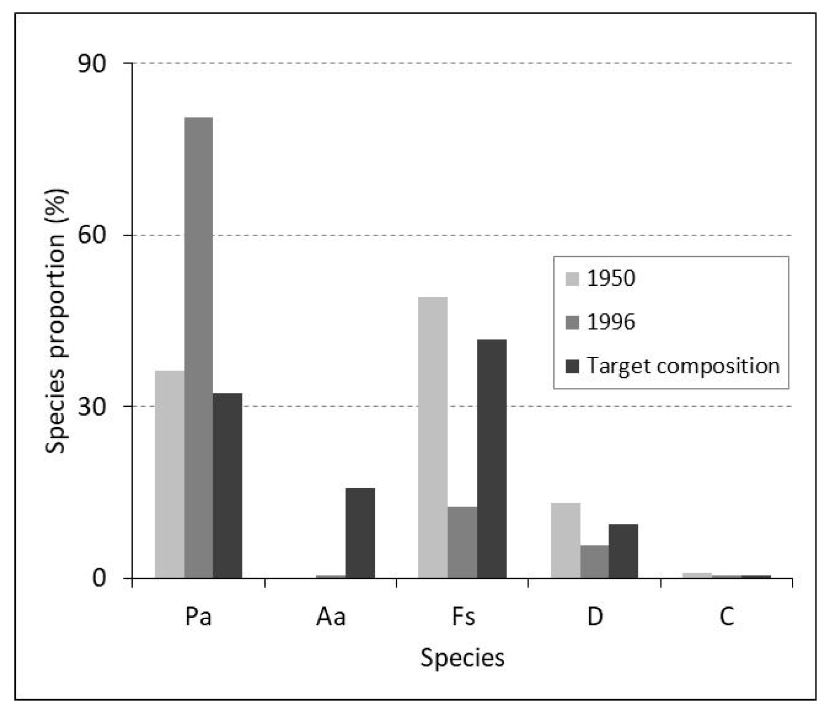
The analysis conducted at the level of management unit IV Tămașu shows that during the period from 1950–1996, the proportion of spruce increased by 44.1% as a result of plantations carried out within the area of mixed beech–coniferous formations and beech forests. The area covered by beech, on the other hand, decreased by 36.6%. Of the total area occupied by spruce, 51% comes from plantations [28]. In the target compositions of forest stands (Table 6), by adopting the compositions of natural forest types, the proportion of fir, beech, and admixed species (sycamore, maple, elm, ash, cherry, goat willow, birch, hornbeam, and others) has been reconsidered. Thus, the forest composition will be richer in species. It will also resemble the composition that existed decades ago (i.e., around 1950) (Figure 5). Research aiming to optimize the future proportion of species must be supplemented with observations on species behavior and conducted during the updating/revision of forest management plans.
4.4. Promoting the Composition of Forest Types through Management Measures
Functional requirements dictate that future stand models must primarily fulfill biodiversity conditions. This is one of the key indicators of sustainable forest management [37]. Dynamics of the composition from Figure 5 show that the natural diversity of species can be influenced in managed forests. It follows that in the studied area, knowledge of forest types is crucial for each forest, and management measures should aim to achieve their composition. For the studied area, management measures should aim to maintain spruce and other species (such as arolla pine, mountain pine, juniper, mountain ash, and green alder) in the composition of forests in the FSA altitude zone (above 1750 m altitude). On avalanche corridors, site conditions are favorable for maintaining spruce with green alder and juniper. In the FM3 zone (altitude 1450–1750 m), it is necessary to preserve spruce as the predominant species. Other coniferous species such as fir and arolla pine may also be introduced in a limited proportion (10%–20%). Depending on the ecological conditions, deciduous species such as beech, sycamore, mountain ash, grey alder, and fir can be maintained dispersed, with fir primarily on sunny slopes. At the lower limit of the FM3 zone, fir, beech, mountain ash, and sycamore can make up to 30% of the stand composition, and this proportion increases as altitude decreases towards the boundary with the mixed forests zone. The most favorable conditions for these species are mainly found on sunny slopes. In the FM2 zone (altitude 1000–1450 m), the proportion of conifers in the stand composition begins to decrease, reaching at most 40% at the lower part of the zone (altitude 1000–1100 m). In the stands in the FM1 + FD4 zone (altitude 800–1000 m), within the beech formation, conifers are maintained at a maximum of 20%. In the same proportion, other deciduous species such as sycamore, maple, elm, ash, and cherry are introduced. However, beech is maintained at a proportion of 70%–80%. Additionally, consideration is provided to other accompanying species such as various deciduous or grey alder in humid sites along valleys and in ravine areas [8].
4.5. Increasing the Functional Efficiency of the Forest
The implementation of forest-type compositions alone is not the only measure for increasing the functional efficiency of forests. Natural regeneration of locally sourced species and diversification of stand structure in the vertical plane become prerequisites for increasing stand stability. In situations where the forest consists of stands with even-aged structures, achieving a balance in age–classes is necessary. This would ensure that the annual growth of the forest remains at the same level, leading to continuous and consistent harvests. This is because, in forests intended for production, the volume of harvests corresponds to the rate of growth. Additionally, timber harvests are obtained from exploitable stands, and in a well-managed forest, the percentage of exploitable stands remains constant. It follows that under the assumption of a management approach that mitigates the effects of climate change [44], the normal structure of the forest ensures a balance of the growing stock throughout the cycle and annual growth, thereby maintaining relatively constant carbon stored in the growing stock. In this study, the carbon stored in the growing stock is 45.2 tha−1, which is consistent with the values determined in other research for forests in the temperate zone [45,46] and is expected to increase to 55.8 tha−1 through improved management practices (Table 5). This involves measures to increase biodiversity, improve stand density, and normalize age structure, as it is common knowledge that a reduction in biodiversity could lead to a decrease in the forest’s capacity to provide ecosystem services [47]. Moreover, meeting these requirements creates favorable conditions for the existence of all biocenotic components of the forest, including for a normal carbon cycle.
5. Conclusions
The research conducted in this study highlights the typological units in a mountainous area where past management has profoundly altered the stand composition and, implicitly, the stand structure. Forest types depend on site conditions, altitude, annual average temperature, exposure, landform, and other ecological factors, determining the proportion of species in the composition of natural ecosystems. Promoting the composition of natural forest types in future stand structures would lead to biodiversity enhancement and, consequently, to achieving key indicators of sustainable forest management. A normal structure in terms of species, age–classes, and stand density facilitates the increase of annually accumulated carbon stock in the growing stock of forests. This implies further improvements in management practices to restore ecosystems with ecologically and functionally damaged structures. The amount of carbon stored both in the growing stock and in forest growth can be defined as an efficiency indicator of applied management. All this information is provided by continuous planning, with each revision opportunity.
Supplementary Materials
The following supporting information can be downloaded at: https://www.mdpi.com/article/10.3390/f15071196/s1, Table S1. Models for estimating the proportion of spruce and beech in relation to site conditions. Table S2. Real values of density and growing stock (m3ha−1) per age–class in the real forest structure. Figure S1. Growing stock per age–class (m3ha−1) when the forest has a normal structure (i.e., age–classes with equal areas), densities of 0.76 and 0.90, and the stands have the composition of forest types (a) and the trend of carbon stock increase when forest structure is normalized and stand composition and density are improved (b). The regression equations in Figure S4a estimate the growing stock of the forest per hectare (e.g., management unit IV Tămaşu) consisting of stands with the compositions of forest types according to age, with an RMSE error ranging from 9.1 to 14.8 m3ha−1 (4.5–5.4%). Figure S4b shows the stored carbon under different structure conditions: 1—real structure; 2—forest with real structure and real density (0.76) but consisting of stands with the composition of natural forest types; 3—forest with normal age–class structure and average density of 0.9, consisting of stands with the composition of natural forest types.
Funding
This research received no external funding.
Data Availability Statement
Data are contained within the article and Supplementary Materials.
Acknowledgments
The author would like to thank I.N.C.D.S. “Marin Drăcea” for allowing access to the forest database. This paper is based on results obtained from a study conducted in 2014 within the framework of the project Ecological restoration of forests in the Făgăraş Mountains, undertaken at Transylvania University of Braşov.
Conflicts of Interest
The author declares that they have no known competing financial interests or personal relationships that could have appeared to influence the work reported in this paper.
References
- Spittlehouse, D.; Stewartz, R. Adaptation to climate change in forest management. BC J. Ecosyst. Manag. 2003, 4, 12–13. [Google Scholar] [CrossRef]
- Bernier, P.; Shoene, D. Adapting forests and their management to climate change: An overview. Unasylva 2009, 60, 5–11. [Google Scholar]
- Blate, G.M.; Joyce, L.A.; Littell, J.S.; McNulty, S.G.; Millar, C.I.; Moser, S.C.; Neilson, R.P.; O’Halloran, K.; Peterson, D.L. Adapting to climate change in Unitated States national forests. Unasylva 2009, 60, 57–60. [Google Scholar]
- Wagner, S.; Nocentini, S.; Huth, F.; Hoogstra-Klein, M. Forest Management Approaches for Coping with the Uncertainty of Climate Change: Trade-Offs in Service Provisioning and Adaptability. Ecol. Soc. 2014, 19, 32. [Google Scholar] [CrossRef]
- Hanewinkel, M.; Cullmann, D.A.; Schelhaas, M.J.; Nabuurs, G.J.; Zimmermann, N.E. Climate change may cause severe loss in the economic value of European forest land. Nat. Clim. Chang. 2013, 3, 203–207. [Google Scholar] [CrossRef]
- Stanturf, J. What is forest restoration? In Restoration of Boreal and Temperate Forests; Stanturf, J., Palle Madsen, P., Eds.; CRC Press: Boca Raton, FL, USA, 2005; pp. 3–11. [Google Scholar]
- Stanturf, J.; Palik, B.; Dumroese, R.K. Contemporary forest restoration: A review emphasizing 633 function. For. Ecol. Manag. 2014, 331, 292–323. [Google Scholar] [CrossRef]
- Tudoran, G.M.; Zotta, M. Adapting the planning and management of Norway spruce forests in mountain areas of Romania to environmental conditions including climate change. Sci. Total Environ. 2020, 698, 133761. [Google Scholar] [CrossRef] [PubMed]
- Armăşescu, S. Cercetări Asupra Producţiei, Creşterii şi Calităţii Arboretelor de Molid (Research on the Production, Growth and Quality of Spruce Stands); Centrul de Documentare Tehnică Pentru Economia Forestieră: Bucharest, Romania, 1965; pp. 26–31. [Google Scholar]
- Ovreiu, A.B.; Oprea, C.R.; Andra-Tpârceanu, A.; Pintilii, R.A. Dendrogeomorphological Reconstruction of Rockfall Activity in a Forest Stand, in the Cozia Massif (Southern Carpathians, Romania). Forests 2024, 15, 122. [Google Scholar] [CrossRef]
- Spathelf, P.; Stanturf, J.; Kleine, M.; Jandl, R.; Chiatante, D.; Bolte, A. Adaptive measures: Integrating adaptive forest management and forest landscape restoration. Ann. For. Sci. 2018, 75, 55. [Google Scholar] [CrossRef]
- Bradshaw, R.H.W. Wat is a natural forest. In Restoration of Boreal and Temperate Forests; Stanturf, J., Palle Madsen, P., Eds.; CRC Press: Boca Raton, FL, USA, 2005; pp. 15–30. [Google Scholar]
- Madsen, P.; Jense, F.A.; Fodgaard, S. Afforestationin Denmark. In Restoration of Boreal and Temperate Forests; Stanturf, J., Palle Madsen, P., Eds.; CRC Press: Boca Raton, FL, USA, 2005; pp. 211–225. [Google Scholar]
- Hahn, K.; Emborg, J.; Bo Larsen, J.; Madsen, P. Forest rehabilitation in Denmark using nature-based forestry. In Restoration of Boreal and Temperate Forests; Stanturf, J., Palle Madsen, P., Eds.; CRC Press: Boca Raton, FL, USA, 2005; pp. 299–317. [Google Scholar]
- Harmer, R.; Thompson, R.; Humphrey, J. Great Britain—Conofers to broadleaves. In Restoration of Boreal and Temperate Forests; Stanturf, J., Palle Madsen, P., Eds.; CRC Press: Boca Raton, FL, USA, 2005; pp. 319–338. [Google Scholar]
- Hansen, J.; Spiecker, H. Conversion of Norway spruce (Picea abies [L] Karst.) forests in Europe. In Restoration of Boreal and Temperate Forests; Stanturf, J., Palle Madsen, P., Eds.; CRC Press: Boca Raton, FL, USA, 2005; pp. 339–347. [Google Scholar]
- Leahu, I. Amenajarea Pădurilor (FOREST Management); Editura Didactică şi Pedagogică: Bucharest, Romania, 2001; pp. 131–135. [Google Scholar]
- Seceleanu, I. Amenajarea Pădurilor. Organizare şi Conducere Structurală (Forest Maangement. Organization and Structural Leadership); Editura Ceres: Bucharest, Romania, 2012; pp. 37–45. [Google Scholar]
- Barbati, A.; Corona, P.; Marchetti, M. A forest typology for monitoring sustainable forest management: The case of European Forest Types. Plant Biosyst.—Int. J. Deal. All Asp. Plant Biol. 2007, 141, 93–103. [Google Scholar] [CrossRef]
- Larsen, J.B.; Nielsen, A.B. Nature-based forest managementwhere are we going? Elaborating forest development types in and with practice. For. Ecol. Manag. 2006, 238, 107–117. [Google Scholar] [CrossRef]
- Corona, P.; Del Favero, R.; Marchetti, M. Stand level forest type approach in Italy: Experiences from the last twenty years. In Monitoring and Indicators of Forest Biodiversity in Europe—From Ideas to Operationality; Marchetti, M., Ed.; European Forest Institute: Joensuu, Finland, 2004. [Google Scholar]
- Jenkins, M.; Schaap, B. Forest Ecosystem Services. Background Analytical Study 1. Global Forest Goals. United Nations Forum on Forests. 2018. Available online: https://www.un.org/esa/forests/wp-content/uploads/2018/05/UNFF13_BkgdStudy_ForestsEcoServices.pdf (accessed on 12 April 2024).
- Li, T.; Wu, C.X.; Wu, Y.; Li, M.Y. Forest Carbon Density Estimation Using Tree Species Diversity and Stand Spatial Structure Indices. Forests 2024, 14, 1105. [Google Scholar] [CrossRef]
- Vilén, T.; Gunia, K.; Verkerk, P.J.; Seidl, R.; Schelhaas, M.J.; Lindner, M.; Bellassen, V. Reconstructed forest age structure in Europe 1950–2010. For. Ecol. Manag. 2012, 286, 203–218. [Google Scholar] [CrossRef]
- Badea, L.; Gastescu, P.; Velce, V.A.; Geografia României, I. Geografia fizică (Geography of Romania. I Physical Geography); Editura Academiei Republicii Socialiste România: Bucharest, Romania, 1983; pp. 90–91. [Google Scholar]
- Bîndiu, C.; Doniţă, N. Molidişurile Presubalpine din România (Subapline Spruce Forests in Roamania); Editura Ceres: Bucharest, Romania, 1988; pp. 15–21. [Google Scholar]
- Spînu, A.P.; Petrițan, I.C.; Mikoláš, M.; Janda, P.; Vostarek, O.; Čada, V.; Svoboda, M. Moderate-to High-Severity Disturbances Shaped the Structure of Primary Picea Abies (L.) Karst. Forest in the Southern Carpathians. Forests 2020, 11, 1315. [Google Scholar] [CrossRef]
- ICAS. Forest Management Planning of Management Units III Cascoe, IV Tămaşu, V Izvoarele Dâmboviţei, V Voina; Insitutul de Cercetări şi Amenajări Silvice: Pitesti, Romania, 1996. (In Romanian) [Google Scholar]
- MAPPM. Norme Tehnice Privind Compoziţii, Scheme şi Tehnologii de Regenerare a Pădurilor şi de Împădurire a Terenurilor Degradate; Ministry of Water, Forests and Environmental Protection: Bucharest, Romania, 2000. [Google Scholar]
- Chiriţă, C.; Vlad, I.; Păunescu, C.; Pătrăşcoiu, N.; Roşu, C.; Iancu, I. Staţiuni Forestiere II (Forest Sites II); Editura Republicii Socialiste România: Bucharest, Romania, 1977; pp. 105–112. [Google Scholar]
- Paşcovschi, S.; Leandru, V. Tipuri de Pădure din Republica Populară Română (Types of Forests in the Romania); Editura Agro-Silvică de Stat: Bucharest, Romania, 1957; pp. 134–135. [Google Scholar]
- Doniţă, N.; Chiriţă, C.D.; Stănescu, V.; Almăşan, H.; Arion, C.; Armăşescu, S. Tipuri de Ecosisteme Forestiere din România (Types of Forest Ecosystems of Romania); Editura Tehnică Agricolă: București, Romania, 1990; 400p. [Google Scholar]
- Coldea, G.; Indreica, A.; Oprea, A. Les Association Végétales de Roumanie, Tome 3, Les Association Forestièr et Arbustives; Presa Universitara Clujană: Cluj, Romania, 2015; 316p. [Google Scholar]
- Reif, A.; Schneider, E.; Oprea, A.; Rakosy, L.; Luick, R. Romania’s natural forest types—A biogeographic and phytosociological overview in the context of politics and conservation [Die natürlichen Waldtypen Rumäniens—Eine biogeographische und vegetationskundliche Übersicht im Kontext von Politik und Naturschutz]. Tuexenia 2022, 42, 9–34. [Google Scholar] [CrossRef]
- Doniţă, N.; Ivan, D.; Coldea, G.; Sanda, V.; Popescu, A.; Chifu, T.; Paucă-Comănescu, M.; Mititelu, D.; Boşcaiu, N. Vegetaţia României (The Vegetation of Romania); Editura Tehnică Agricolă: Bucharest, Romania, 1992; p. 27. [Google Scholar]
- Pătrăşcoiu, N. Proporţia Optimă de Extindere a Speciilor de Răşinoase Pentru Mărirea Productivităţii Pădurilor şi Sporirea Eficienţei în Protecţia Mediului Înconjurător; I.C.A.S.: Bucharest, Romania, 1982; pp. 3–4. [Google Scholar]
- EEA. European Forest Types. Categories and Types for Sustainable Forest Management and Reporting. European Environment Agency, EEA Technical Report No. 9/2006. 2006. 2006. Available online: https://www.eea.europa.eu/publications/technical_report_2006_9 (accessed on 12 June 2022).
- Available online: https://www.meteoblue.com/ro/vreme/archive/windrose/bra%C8%99ov_rom%C3%A2nia_683844 (accessed on 17 March 2022).
- Giurgiu, V.; Decei, I.; Drăghiciu, D. Metode şi Tabele Dendrometrice; Editura Ceres: Bucharest, Romania, 2004; pp. 35–44, 53–54. [Google Scholar]
- IPCC Guidelines for National Greenhouse Gas. Inventories; IPCC: Geneva, Switzerland, 2006; Volume 4, Available online: https://www.ipcc-nggip.iges.or.jp/public/2006gl/vol4.html (accessed on 28 June 2022).
- Goslee, K.; Walker, S.M.; Grais, A.; Murray, L.; Casarim, F.; Brown, S. Module C-CS: Calculations for Estimating Carbon Stocks. In Leaf Technical Guidance Series for the Development of a Forest Carbon Monitoring System for REDD+; Winrock International: Little Rock, AR, USA, 2016. [Google Scholar]
- Larsen, J.B. Ecological stability of forests and sustainable silviculture. For. Ecol. Manag. 1995, 73, 85–96. [Google Scholar] [CrossRef]
- Barbati, A.; Marchetti, M.; Chirici, G.; Corona, P. European Forest Types and Forest Europe SFM indicators: Tools for monitoring progress on forest biodiversity conservation. For. Ecol. Manag. 2014, 321, 145–157. [Google Scholar] [CrossRef]
- Kindermann, G.E.; Schörghuber, S.; Linkosalo, T.; Sanchez, A.; Rammer, W.; Seidl, R.; Lexer, M.J. Potential stocks and increments of woody biomass in the European Union under different management and climate scenarios. Carbon Balance Manag. 2013, 8, 2. [Google Scholar] [CrossRef] [PubMed] [PubMed Central]
- Malhi, Y.; Baldocchi, D.D.; Jarvis, P.G. The carbon balance of tropical, temperate and boreal forests. Plant Cell Environ. 1999, 22, 715–740. [Google Scholar] [CrossRef]
- Forest Europe. State of Europe’s Forests 2020. 2020. Available online: https://foresteurope.org/wp-content/uploads/2016/08/SoEF_2020.pdf (accessed on 4 March 2024).
- Brockerhoff, E.G.; Barbaro, L.; Castagneyrol, B.; Forrester, D.L.; Gardiner, B.; Gonzales-Ollavaria, J.R.; Lyver, P.O.B.; Meurisse, N.; Oxbrough, A.; Taki, H.; et al. Forest biodiversity, ecosystem functioning and the provision of ecosystem services. Biodivers Conserv. 2017, 26, 3005–3035. [Google Scholar] [CrossRef]
Figure 1.
Map of the research area (green—spruce stands; yellow—mixed stands; brown—beech stands) [8].
Figure 1.
Map of the research area (green—spruce stands; yellow—mixed stands; brown—beech stands) [8].
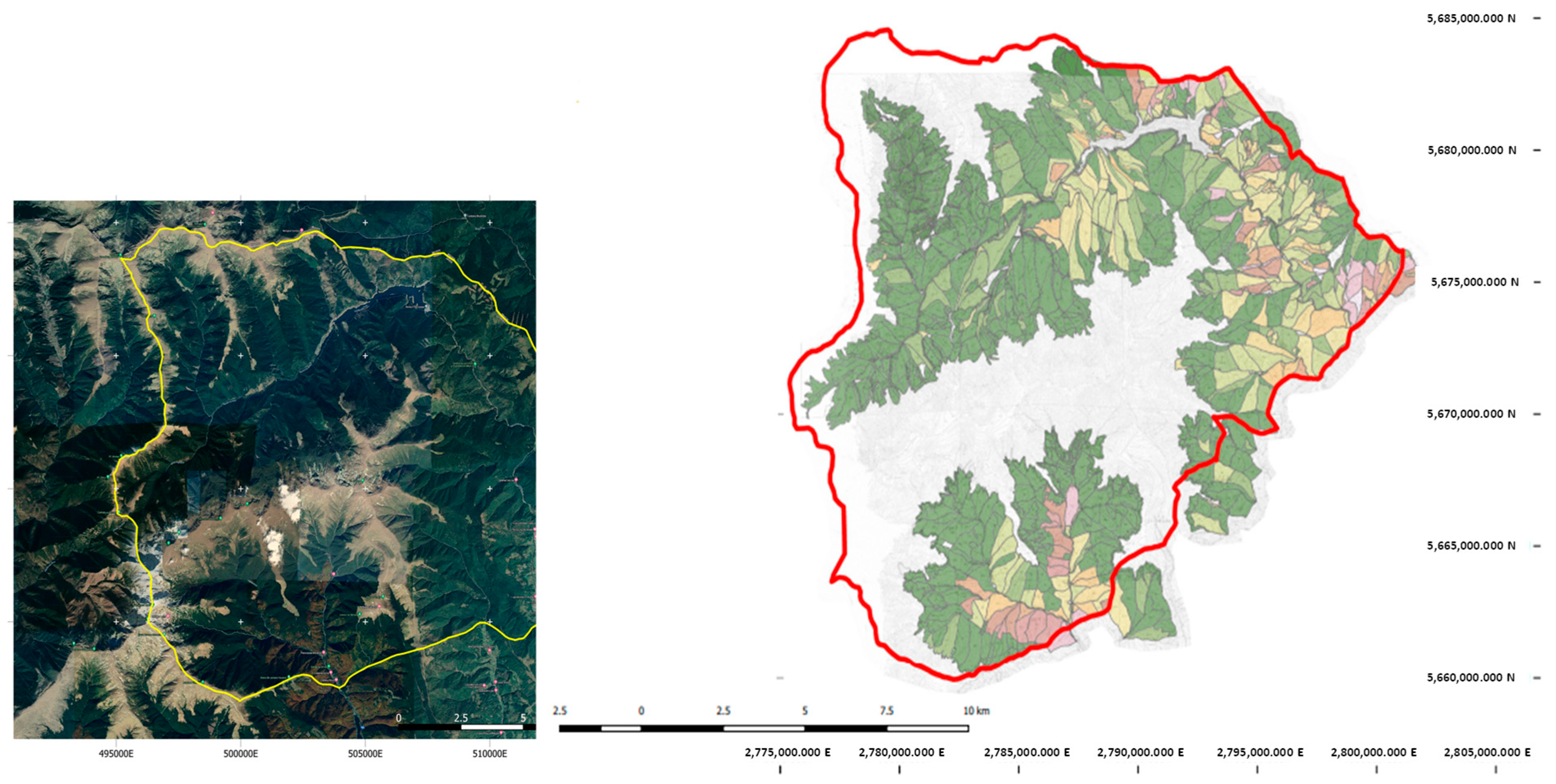
Figure 2.
The natural distribution of deciduous species (a) and conifers (b) in relation to altitude. The trend of the proportion of the two groups of species (i.e., deciduous—D and coniferous—C) can be expressed by the equations: DP = –53.082 A4 + 384.4 A3 – 971 A2 + 907.3 A – 185.1 and CP = –62.718 A4 + 113.03 A3 + 138.11 A2 – 234.62 A + 70. Altitude explains 38%–50% of the variation in the proportion of the two species groups. Spruce from plantations was not included in the equation.
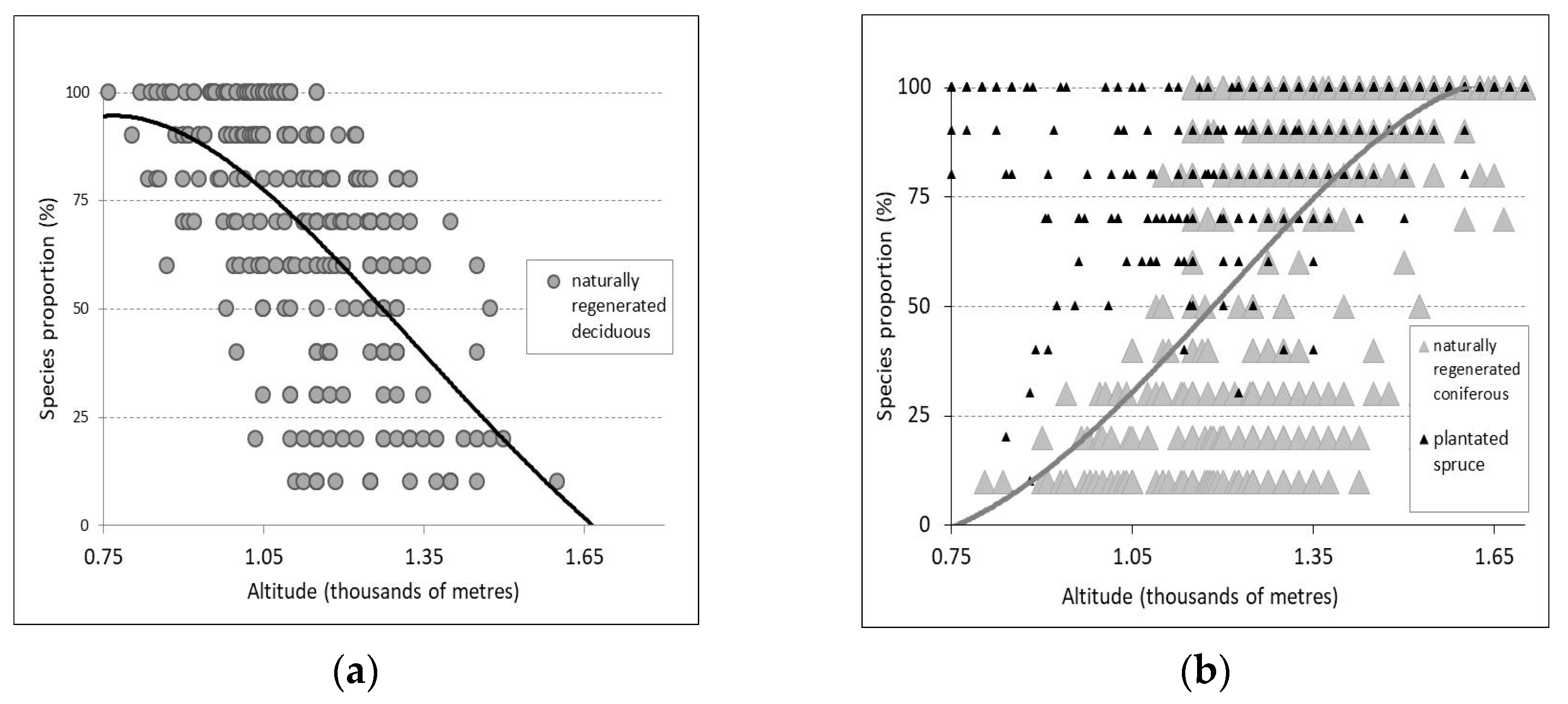
Figure 3.
The relation between species proportion and altitude for (a) spruce and fir, on sunny (S and SW) and shaded (N and NE) slopes, and (b) variation of stand composition in relation to altitude, on sunny slopes (S and SW). On sunny slopes, the species proportion varies with altitude as follows: Spruce, P = 104.38 A3 − 42.857 A 2 − 226.8 A + 166.4 (1000–1400 m), P = –426.97 A2 + 1470.1 A − 1170.5 (1401–1850 m); Fir, P = –784.51 A3 + 2367.1 A2 − 2278.5 A + 710.21 (850–1200 m), P = 969.7 A3 − 4105.8 A2 + 5689.8 A − 2562 (1201–1600 m); Arolla pine, P = 146.43 A2 − 470.89 A + 380.84 (1650–1850 m); Beech, P = 264.49 A3 − 987.94 A2 + 1093.4 A − 297.76 (800–1400 m), P = 666.67 A3 − 2842.9 A2 + 3921.9 A − 1725.5 (1401–1600 m); Deciduous species, P = –65.254 A3 + 260.32 A2 − 348.24 A + 165.75 (800–1400 m), P = 217.4 A3 − 1056.4 A2 + 1679.9 A − 868.57 (1401–1800 m). The equations estimate the average proportion of species at the forest formation level. Extra-zonal spruce was not considered for the generation of the equations.

Figure 4.
The forest structure—real and normal—by 20-year age–class distribution for a 120-year production cycle (a), and the carbon stored by age–class when the forest has both real age–class structure and a normal structure (b). In the normal structure, the age–classes are equal in area (as in (a)), the stands have compositions identical/similar to those of forest types, and their density is 0.9. In the real (current) structure, the forest has real areas per age–class, compositions, and densities (the areas per age–class are as in (b), and the forest has an average density of 0.76). These details are specific to management unit IV Tămaşu with an area of 4303.2 ha.
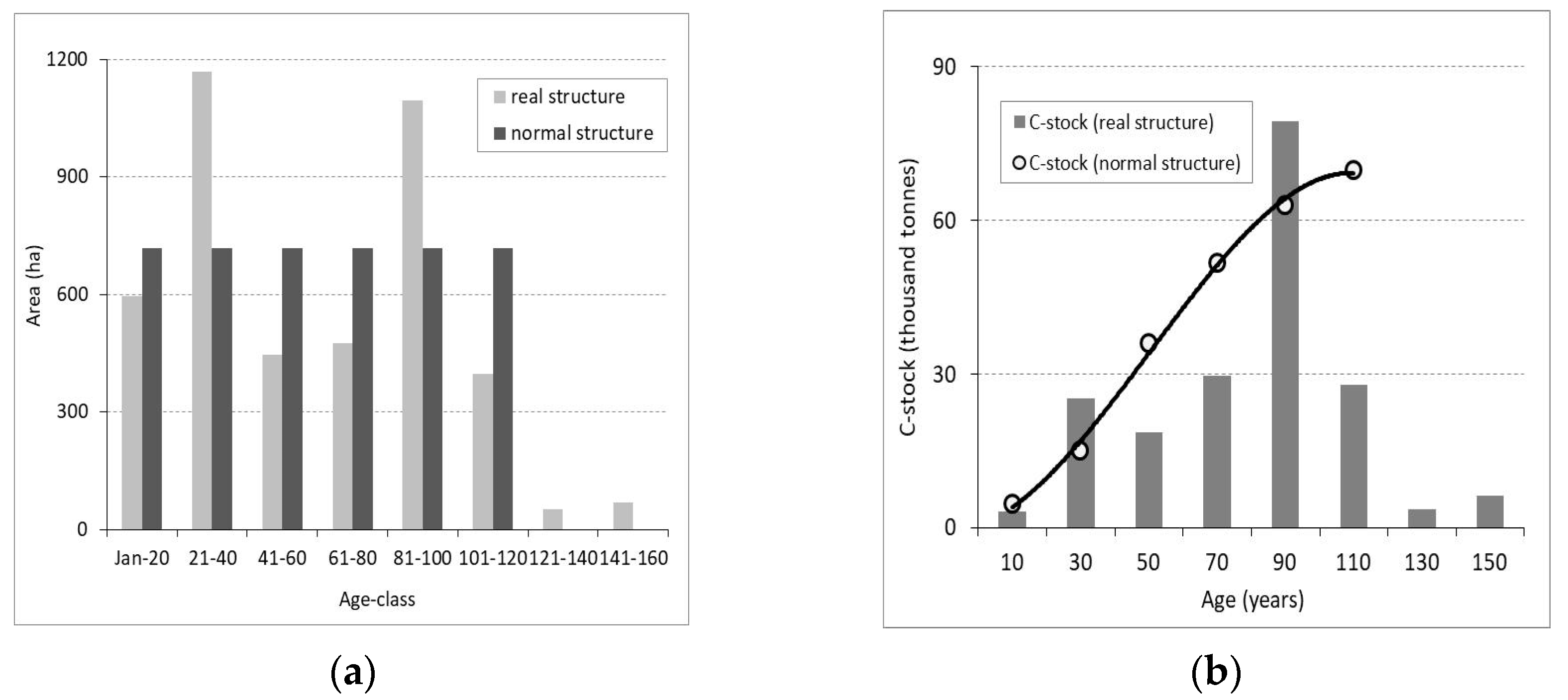
Figure 5.
Forest composition dynamics in the Tămașu management unit. Species: Ps—spruce, Aa—fir, Fs—beech, D—other deciduous species, C—other coniferous species.
Figure 5.
Forest composition dynamics in the Tămașu management unit. Species: Ps—spruce, Aa—fir, Fs—beech, D—other deciduous species, C—other coniferous species.

Table 1.
Characteristics for key areas.
| Management Unit | III Cascoe | IV Tămaşu | V Izvoarele Dâmboviţei | V Voina | Total | |||||||
|---|---|---|---|---|---|---|---|---|---|---|---|---|
| Area (ha) | 7.9 | 282.9 | 308.6 | 541.2 | 1140.6 | |||||||
| Altitude (m)/Exposure | N, NE | S, SW | E, SE, W, NW | Total | ||||||||
| 900–1400 | 5 | 16 | 21 | 42 | ||||||||
| 1450–1550 | 7 | 9 | 16 | 32 | ||||||||
| 1600–1800 | 4 | 3 | 18 | 25 | ||||||||
| 1850–1900 | – | – | 1 | 1 | ||||||||
| Total | 16 | 28 | 56 | 100 | ||||||||
| Inclination (°) | 0–15 | 16–25 | 26–30 | 31–35 | 36–40 | 41–45 | Total | |||||
| Area (%) | 1 | 5 | 14 | 50 | 28 | 2 | 100 | |||||
| Age class | I | II | III | IV | V | VI | VII | VIII | Regeneration class | Total | ||
| Area (ha) | 17.5 | 125.7 | 309.8 | 208.6 | 283.9 | 112.9 | 71.0 | 8.6 | 2.6 | 1140.6 | ||
| Species | Pa | Fs | Aa | Ai | Od | Regeneration class | Total | |||||
| Area (ha) | 1091.6 | 34.1 | 7.5 | 1.8 | 3.0 | 2.6 | 1140.6 | |||||
Pa—Picea abies (L.) Karst., Norway spruce; Fs—Fagus sylvatica L., European beech; Aa—Abies alba Mill., Silver fir; Ai—Alnus incana (L.), Moench., Grey alder; Od—Other deciduous species. Data from a study conducted in 2014 within the framework of the project Ecological restoration of forests in the Făgăraş Mountains, undertaken at Transylvania University of Braşov.
Table 2.
Distribution of zonal units in the Upper Dâmbovița Valley watershed, Făgăraș Mountains.
| Zonal Unit by Altitude | Bioclimatic Zonal Units | Features of Typological Units | ||||
|---|---|---|---|---|---|---|
| zone | Subzone | Phytoclimatic zone | Subzone | Formation of forest types | Altitude | |
| Shady slopes | Sunny slopes | |||||
| Subalpine | - | Subalpine (FSA) | - |
| From 1750 (1800) to 1700 (1750) m | From 1880 (1900) to 1800 (1850) m |
| Boreal (spruce forests) | - | Mountain spruce forests (FM3) | Upper mountain (pre-subalpine) |
| From 1750 to 1550 m | From 1850 to 1650 (1600) m |
| Middle mountain |
| From 1550 to 1450 m | From 1650 to 1550 m | |||
| Nemoral (deciduous forests) | Beech and mixed forests | Mixed mountain forests (FM2) |
| From 1450 to 1200 m | From 1550 to 1250 m | |
| Lower mountain |
| From 1200 to 1000 m | From 1250 to 1100 m | |||
| Mountain and pre-mountain beech forest (FM1 + FD4) |
| From 950–1000 to 800 m | From 1050–1100 to 800 m | |||
The classification of tipological units was adapted to the scheme of vegetation zones in Romania [35]. The formation of forest types includes all types of forests composed of the same species or combination of woody species. Forest types within a formation can have different productivities, and the types of indicator plants within the formation can also vary (i.e., spruce forests with Vaccinium, spruce forests with Oxalis).
Table 3.
Natural forest types and target compositions.
| Site Type | Natural Forest Type | Characteristics/Spread | Species | Target Composition (the Proportion of the Species Is Expressed in Tenths) |
|---|---|---|---|---|
| 11 Spruce forests (FSA and FM3) | ||||
| 1120. Subalpine, low productivity, podzolic | 1161. Spruce open forest with arolla pine (Pinus cembra) | At the limit of mountain pine (Pinus mugo) forests Altitude 1750–1850 (1900) m Coverage 10%–50% | Pa ± Pc, Sa, Pm, Jc, Av | 8–9 Pa, 1–2 Pc ± Sa, Pm, Jc, Av |
| 1510. Subalpine on avalanche corridors, low productivity, podzolic | 1181. Spruce open forest with green alder on avalanche corridors | On avalanche corridors | Pa ± Sa, Av, Pm, Jc | 6–8 Pa, 2–4 Av, Sa |
| 1210. Spruce mountain pre-subalpine, low productivity, peat soil with Vaccinium, Polytrichum | 1154. Spruce forest at altitudinal limit with Vaccinium | At the limit of mountain pine (Pinus mugo) forest Altitude 1700–1750 m | Pa ± Pc, Sa, Pm, Jc | 8–9 Pa, 1–2 Pc ± Sa, Pm, Jc |
| 1320. Spruce mountain pre-subalpine, low productivity, podzolic with Vaccinium | 1152. Spruce forest at altitudinal limit with Vaccinium mirtillus and Oxalis acetosella | Pre-subalpine spruce forest at altitudinal limit Altitude 1600–1850 m | Pa ± Pc, Sa, Pm, Jc | 8–9 Pa, 1–2 Pc ± Sa, Pm, Jc |
| 1330. Spruce mountain pre-subalpine, low productivity, podzolic with Oxalis, Soldanella | 1122. Spruce forest with green moss | On predominantly shaded/northern slopes Altitude 1600–1750 m | Pa ± Pc, Sa, Pm | 8–9 Pa, 1–2 Pc ± Sa, Pm, Av |
| 2120. Spruce mountain, rocky | 1162. Spruce forest on rock | On slopes with rocks and boulders on the surface Altitude 1600–1750 m | Pa ± Pc, Sa, Pm, Jc, Av | 7–8 Pa, 2–3 Pc ± Sa, Pm, Jc, Av |
| 2311. Spruce mountain, low productivity, podzolic with Vaccinium | 1153. Spruce forest with Vaccinium mirtillus | Altitude 1400–1500 (1600) m | Pa ± Aa, Ps (Pc, Ps), Fs, App, Sa, Ai | 7–8 Pa, 2–3 Aa, Fs, App, Ps ± Sa, Ai (at the upper limit) 7–8 Pa, 1–2 Aa (Pc, Ps), 1 Fs, App, Sa, Ai (at the lower limit) |
| 2312. Spruce mountain, medium productivity, podzolic | 1151. Spruce forest with Vaccinium mirtillus and Oxalis acetosella | On shaded and semi-shaded slopes Altitude 1350–1600 m | Pa ± Aa, Ps (Pc, Ps), Fs, App, Sa, Ai | 7–8 Pa, 2–3 Aa (Pc, Ps) + Fs, App, Sa, Ai (at the upper limit) 7–8 Pa, 1–2 Aa (Ps), 1 Fs, App, Sa (at the lower limit) |
| 2332. Spruce mountain, medium productivity, brown with moder–mull | 1113. High altitude spruce forest with Oxalis acetosella | Altitude 1300–1650 m | Pa ± Aa, Ps (Pc), Fs, App, Sa, Ai | 7–8 Pa, 2–3 Aa (Pc) + Fs, App, Sa, Ai (at the upper limit) 6–8 Pa, 1–2 Aa, 1–2 Fs, App, Sa, Ai (at the lower limit) |
| 1114. Spruce forest on skeletal soil with Oxalis acetosella | Altitude 1300 –1550 (1600) m | Pa ± Aa, Ps, Fs, App, Fe, Sa, Ai | 7–8 Pa, 2–3 Aa (Ps), 1 Fs, App, Sa, Ai (at the upper limit) 7–8 Pa, 1–2 Aa (Pc, Ps), 1–2 Fs, App, Fe, Sa (at the lower limit) | |
| 14 Beech–spruce forests (FM2) | ||||
| 3311. Mixed mountain, medium productivity, with Vaccinium and other acidophiles | 1421. Beech–spruce forest with Vaccinium myrtillus and Oxalis acetosella | On shaded slopes. Altitude 1350–1450 m | Pa, Fa, Aa ± App, Sa, Ug, Bp | 4–6 Pa, 3–4 Fs, App, 1–2 Aa ± Sa, Bp |
| 3321. Mixed mountain, low productivity, brown podzolic with Luzula ± Calamagrostis | 1431. Beech–spruce forest with Luzula luzuloides | On sunny slopes Altitude 1200–1400 m | Pa, Aa, Fs ± App, Ap, Fe, Sa, Bp | 4–6 Pa, 2–3 Aa, 2–3 Fs, App, Ap ± Sa, Bp (at the upper limit) 4–5 Pa, Aa, 5–6 Fs, App, Ap, Bp (in the other sites) |
| 1.3 Mixed coniferous-beech forests (spruce–fir–beech) (FM2) | ||||
| 3322. Mixed mountain, medium productivity, acid with moder | 1331. Mixed coniferous-beech forest with Festuca altissima | On shaded and semi-sunny slopes Altitude 1000–1400 m | Pa, Aa, Fs ± App, Ap, Fe, Sa, Bp | 4–5 Pa, 2–3 Aa, 3 Fs, App, Ap ± Sa, Bp (at the upper limit) 2–3 Pa, 2–3 Aa, 4–6 Fs, App, Ap ± Fe, Bp (in the other sites) |
| 3332. Mixed mountain, medium productivity, brown with mull | 1341. Mixed coniferous-beechforest on skeletal soils | On sunny and semi-sunny slopes with shallow soil Altitude 1000–1300 (1400) m | Pa, Aa, Fs ± App, Ap, Fe, Ug | 3–4 Pa, 3 Aa, 3–4 Fs, App, Ap (at the upper limit) 2–3 Pa, 2–3 Aa, 4–6 Fs, App, Ap ± Fe, Ug (in the other sites) |
| 41 Beech forests (FM1 + FD4) | ||||
| 4322. Common beech mountain, premontane, medium productivity, brown with mull | 4114. Mountain beech forest on skeletal soils with mull plants | Altitude 800–900 m on slopes with different exposures Altitude 1000–1200 m on sunny and semi-sunny slopes | Fa, Aa, Pa ± App, Ap, Fe, Pav, Ug, Cb | 8–9 Fs, 1–2 Aa (Pa), App, Ap ± Ug, Fe, Pav, Cb |
| 4332. Common beech mountain, premontane, medium productivity, podzolic with Festuca | 4141. Mountain beech forest with Festuca altissima | On sunny and semi-sunny slopes Altitude 1000–1200 m | Fs, Aa, Pa ± App, Ap, Fe, Pav, Ug | 7–8 Fs, 2–3 Aa, Pa, App, Ap ± Ug, Fe, Pav |
| 4331. Common beech mountain, premontane, lower productivity, podzolic with Luzula, Calamagrostis | 4151. Mountain beech forest with Luzula albida | Altitude 1000–1400 m on slopes with different exposures | Fs, Aa, Pa ± App, Ap, Fe, Ug, Bp | 7–8 Fs, 2–3 Aa, Pa ± App, Ap, Ug, Bp |
| 98 Alder (grey alder) forests | ||||
| 3730. Mixed mountain, medium productivity, alluvial | 9811. Grey alder forest with Oxalis acetosella | In valleys Altitude 800–1700 m | Ai ± Pa, Aa, Fe, App | 8–10 Ai, 1–2 Pa, Aa, App |
In its name, the type of site includes the orographic region and its subdivisions suitable for the forest formation, the productive potential for the respective formation, the genetic soil type with indications on the useful physiological regime, and the indicator species from the soil flora [30]. In the name of the natural forest type, the group of formations, forest formation, type of indicator plants, and productivity of the forest type are included. The target composition was established based on the combination of species from the researched ecosystems. Also considered were target compositions recommended by the technical guidelines [29], with adaptations to the specific ecological conditions of the studied area. The proportion of species in the target stand composition is expressed in units from 1 to 10. Pa—Norway spruce, Picea abies (L.) Karst.; Pc—Arolla pine, Pinus cembra L.; Sa—European mountain ash, Sorbus aucuparia L.; Pm—mountain pine, Pinus mugo Tura; Jc—common juniper, Juniperus communis L.; Av—green alder, Alnus viridis (D. C.) Chaix.; Aa—silver fir, Abies alba Mill.; Ps—Scots pine, Pinus sylvestris L.; Fs—European beech, Fagus sylvatica L.; App—sycamore, Acer pseudoplatanus L.; Ap—Norway maple, Acer platanoides L.; Ai—grey alder, Alnus incana (L.) Moench.; Fe—European ash, Fraxinus excelsior L.; Ug—wych elm, Ulmus glabra Huds.; Bp—silver birch, Betula pendula Roth; Pav—wild cherry, Prunus avium L.; Cb—hornbeam, Carpinus betulus L. From the analysis of the typological units shown in Table 3, it appears that several forest habitat types are widespread in the study area: 9420 Alpine Pinus cembra forests; 9410 Montane to alpine acidophilous Picea forests (Vaccinio–Piceetea); 9110 Luzulo–Fagetum beech forests (including mixtures of beech with fir and spruce, and pure beech forests with the same type of acidophilous plants/flora); 91V0 Dacian beech forests (Symphyto–Fagion) (including natural forest types 1331, 1341 and 4114); 91E0 Alluvial forests with Alnus incana (Alnion incanae) (including forest type 9811, found in meadows and wetlands at the base of slopes).
Table 4.
Values of the proportion of species in relation to altitude.
| Altitude (m) | Proportion sf Species (%) | |||||
|---|---|---|---|---|---|---|
| Ps | Aa | Pc | Fs | Od | Total | |
| 900 | - | 5 | - | 80 | 15 | 100 |
| 1050 | 2 | 20 | - | 66 | 12 | 100 |
| 1200 | 13 | 29 | - | 48 | 10 | 100 |
| 1350 | 40 | 22 | - | 29 | 0 | 100 |
| 1500 | 73 | 8 | - | 12 | 7 | 100 |
| 1650 | 93 | - | 3 | - | 4 | 100 |
| 1800 | 92 | - | 7 | - | 1 | 100 |
Ps—spruce, Aa—fir, Pc—Arolla pine, Fs—beech, Od—other deciduous species. At the same altitude, the proportion of species can differ depending on forest type. At altitudes between 900 and 1000 m, the proportion of spruce has decreased, giving way to a higher proportion of fir, which is better adapted to the site conditions in the studied area.
Table 5.
The relation between forest structure conditions and carbon stock.
| Forest Structure by Age–Class | Forest Composition | Average Density | Growing Stock(m3ha−1) | Carbon Stock (tha−1) |
|---|---|---|---|---|
| Real | 80% Pa 12% Bp 5% Od 1% Oc | 0.76 | 251 | 45.2 |
| Real | 42% Fs 33% Pa 15% Aa 5% Od 4% App 1% Pc | 0.76 | 237 | 50.1 |
| Normal | 42% Fs 33% Pa 15% Aa 5% Od 4% App 1% Pc | 0.90 | 275 | 55.8 |
The forest composition of 80% Pa 12% Bp 5% Od 1% Oc is the real (i.e., current) one, while the composition of 42% Fs 33% Pa 15% Sf 5% Od 4% App 1% Pc corresponds to forest types (i.e., normal). Even though at the level of the real composition, the average volume per hectare is higher than in the equivalent natural forest types, the carbon stock is lower due to the high percentage of conifers.
Table 6.
Target compositions for stands in the Tămașu management unit.
| Forest Type (Code) | Altitude (m) | Exposure | Area (ha) | Target Composition |
|---|---|---|---|---|
| 41 Beech forests | ||||
| 4141; 4114 | 900–1000 | S, SW | 292.3 | 80% Fs 10% Aa 10% App, Ap, Fe, Ug, Pav, Cb, Bp, Sa |
| 900–1050 | E, SE, V, NV | 285.1 | 80% Fs 10% Aa, Pa 10% App, Ap, Fe, Ug, Pav, Cb, Bp, Sa | |
| 900–1000 | N, NE | 130.6 | 80% Fs 10% Pa, Aa 10% App, Ug, Pav, Cb, BpSa | |
| 13 Mixed beech–coniferous forest | ||||
| 1331; 1341 | 1150–1500 | S, SV | 1098.3 | 50% Fs 20% Pa 20% Aa 10% App, Ap, Bp, Sa |
| 1100–1450 | E, SE, V, NV | 1310.9 | 40% Fs 30% Pa 20% Aa 10% App, Ap, Bp, Sa | |
| 1050–1400 | N, NE | 321.6 | 40% Pa 30% Fs 20% Aa 10% App, Bp, Sa | |
| 11 Spruce forest | ||||
| 1113; 1151; 1153; 1114 | 1450–1600 | E, SE, S, SV, V, NV | 593.9 | 70% Pa 10% Aa 10% Fs 10% App, Sa |
| 1550–1600 | N, NE | 22.3 | 80% Pa 10% Aa, Pc 10% App, Fs, Sa | |
| 1152 | 1650–1750 | all exposures | 228.7 | 90% Pa 10% Pc + Sa, Pm, Av |
| 1161 | 1800–1850 | all exposures | 18.6 | 80% Pa 20% Pc + Sa, Pm, Jc, Av |
| 9.8 Alder (grey alder) forests | ||||
| 9821 | 960 | - | 0.9 | 80% Ai 20% Pa, Aa, App |
| Total | 4303.2 | - | ||
Species: Pa—Norway spruce, Picea abies (L.) Karst.; Pc—Arolla pine, Pinus cembra L.; Sa—European mountain ash, Sorbus aucuparia L.; Pm—mountain pine, Pinus mugo Tura; Jc—common juniper, Juniperus communis L.; Av—green alder, Alnus viridis (D. C.) Chaix.; Aa—Silver fir, Abies alba Mill.; Fs—European beech, Fagus sylvatica L.; App—sycamore, Acer pseudoplatanus L.; Ap—Norway maple, Acer platanoides L.; Ai—grey alder, Alnus incana (L.) Moench.; Fe—European ash, Fraxinus excelsior L.; Ug—wych elm, Ulmus glabra Huds.; Bp—silver birch, Betula pendula Roth; Pav—wild cherry, Prunus avium L.; Cb—hornbeam, Carpinus betulus. L.
Disclaimer/Publisher’s Note: The statements, opinions and data contained in all publications are solely those of the individual author(s) and contributor(s) and not of MDPI and/or the editor(s). MDPI and/or the editor(s) disclaim responsibility for any injury to people or property resulting from any ideas, methods, instructions or products referred to in the content. |
© 2024 by the author. Licensee MDPI, Basel, Switzerland. This article is an open access article distributed under the terms and conditions of the Creative Commons Attribution (CC BY) license (https://creativecommons.org/licenses/by/4.0/).
Share and Cite
MDPI and ACS Style
Tudoran, G.-M. Composition of Natural Forest Types—Long-Term Goals for Sustainable Forest Management. Forests 2024, 15, 1196. https://doi.org/10.3390/f15071196
AMA Style
Tudoran G-M. Composition of Natural Forest Types—Long-Term Goals for Sustainable Forest Management. Forests. 2024; 15(7):1196. https://doi.org/10.3390/f15071196
Chicago/Turabian StyleTudoran, Gheorghe-Marian. 2024. "Composition of Natural Forest Types—Long-Term Goals for Sustainable Forest Management" Forests 15, no. 7: 1196. https://doi.org/10.3390/f15071196
Note that from the first issue of 2016, this journal uses article numbers instead of page numbers. See further details here.