Incorporating Spatial Autocorrelation into GPP Estimation Using Eigenvector Spatial Filtering

Abstract

Terrestrial gross primary productivity (GPP) is a critical part of land carbon fluxes. Accurately quantifying GPP in terrestrial ecosystems and understanding its spatiotemporal dynamics are essential for assessing the capability of vegetation to absorb carbon from the atmosphere. Nevertheless, traditional remote sensing estimation models often require complex parameters and data inputs, and they do not account for spatial effects resulting from the distribution of monitoring sites. This can lead to biased parameter estimation and unstable results. To address these challenges, we have raised a spatial autocorrelation light gradient boosting machine model (SA-LGBM) to enhance GPP estimation. SA-LGBM combines reflectance information from remote sensing observations with eigenvector spatial filtering (ESF) methods to create a set of variables that capture continuous spatiotemporal variations in plant functional types and GPP. SA-LGBM demonstrates promising results when compared to existing GPP products. With the inclusion of eigenvectors, we observed an 8.5% increase in R² and a 20.8% decrease in RMSE. Furthermore, the residuals of the model became more random, reducing the inherent spatial effects within them. In summary, SA-LGBM represents the first attempt to quantify the impact of spatial autocorrelation and addresses the limitations of underestimation present in existing GPP products. Moreover, SA-LGBM exhibits favorable applicability across various vegetation types.

1. Introduction

Terrestrial gross primary productivity (GPP), serving as a vital metric for carbon assimilation through photosynthesis, constitutes a vital component of terrestrial carbon fluxes [1]. It reflects the ability of plants to absorb atmospheric carbon dioxide and transform it into organic matter [2]. Accurately quantifying GPP and evaluating its dynamic changes are essential for assessing the carbon sink potential of terrestrial ecosystems. Therefore, this endeavor contributes to a deeper understanding of carbon balance, greenhouse gas emissions, and the state of climate change [3,4]. However, the direct observation of GPP poses significant challenges. There are observations obtained from ground-based measurements, spatially scattered sampling, and flux sites, which are only effective within a restricted spatial and time coverage [5]. Therefore, data-driven approaches and simulations facilitated through remote sensing have extended GPP to larger spatial scales. However, whether derived from ground-based observations or data-driven models, the estimation of GPP inevitably faces the influence of environmental variables, the structural complexity of the model, and the diversity of vegetation types. Consequently, in order to mitigate climate change and achieve the aspirations of “carbon peaking” and “carbon neutrality”, enhancing the performance of GPP estimation and bolstering the applicability of the models remain imperative tasks [6].

Remote sensing estimation models have emerged as a predominant tool for assessing GPP, primarily due to their long temporal scales and extensive spatial monitoring capabilities [7]. These models for estimating GPP can roughly be categorized into statistical models, ecological process models, light use efficiency (LUE) models, and machine learning models [5]. Statistical models utilize various commonly employed statistical methods to establish mathematical relationships between changes in plant biomass and climatic factors, aiming to estimate vegetation productivity. These models have simple structures and few parameters, but lack rigorous physiological foundations, resulting in higher uncertainty in the estimation results [8]. Ecological process models employ mechanistic models based on biogeochemical processes. They estimate GPP by modeling processes such as solar radiation transfer and vegetation photosynthesis [9]. These models require complex parameters and comprehensive data inputs [10,11]. The LUE model calculates GPP in view of the link between LUE, absorbed photosynthetically active radiation (APAR), and environmental factors, and integrates physiological and ecological processes inherent to vegetation photosynthesis [12,13,14]. However, variations in the configuration of model parameters can significantly influence the estimation of GPP [15,16,17,18,19]. Machine learning algorithms leverage mathematical and statistical methodologies to analyze datasets and establish intricate associations between input and target variables. This iterative process involves training the model to minimize the loss function. Over the past few years, significant advancements have been achieved in GPP estimation by employing machine learning techniques. These methods utilize data-driven techniques to statistically summarize the relationship between GPP and observed variables [20]. Furthermore, in GPP simulation, machine learning methods have demonstrated effectiveness in reducing uncertainty associated with model parameters, the concrete architecture of models, and input variables, which are inherent in other empirical-based and ecological process-based models [21,22].

Furthermore, the distribution of GPP might be influenced by spatial autocorrelation, where similarities among locations lead to data correlations [23]. When constructing models based on site-level observations, it is often assumed that these sites operate independently, with spatial influences arising from site distribution omitted during modeling. This omission, in turn, results in distorted parameter estimations and outcomes of questionable stability [24,25]. Therefore, a straightforward and efficient methodology that incorporates the spatial effects of variables into the modeling process is required to ensure precise and reliable outcomes. To mitigate the impact of spatial autocorrelation, we employed an eigenvector spatial filter (ESF) approach by incorporating spatial factors that reflect the spatial interdependencies among distinct locations [26]. The core of the ESF methodology revolves around leveraging the neighborhood context of sites to construct the spatial weights matrix that captures the spatial correlation between different sites [27,28]. These weights can be derived from considerations such as distance, orientation, and similarities among sites. Once the spatial weights matrix is formulated, it is used to calibrate parameter estimations within the model, effectively incorporating spatial effects into the estimation model. It has been demonstrated that the application of the ESF approach to machine learning provides more precise predictions [29].

Therefore, this study introduces a GPP remote sensing estimation model that accounts for spatial autocorrelation, denoted as SA-LGBM. SA-LGBM is characterized by its consideration of autocorrelation in the spatial distribution of GPP. Specifically, this work performed three primary tasks: (1) Based on the influencing factors of photosynthesis, a set of model variables capturing GPP changes was selected from remote sensing observations. Using the first law of geography, the spatial weights matrix was constructed to represent relationships between American flux sites, and feature vectors were created and extracted as spatial factors. (2) GPP estimation models were constructed using various machine learning algorithms, evaluating the effect of spatial autocorrelation on the models. The model’s performance was quantitatively evaluated, and comparisons were made with other GPP products. (3) The capacity of the model to be utilized for various vegetation types and the dynamics of GPP were analyzed.

2. Data and Preprocessing

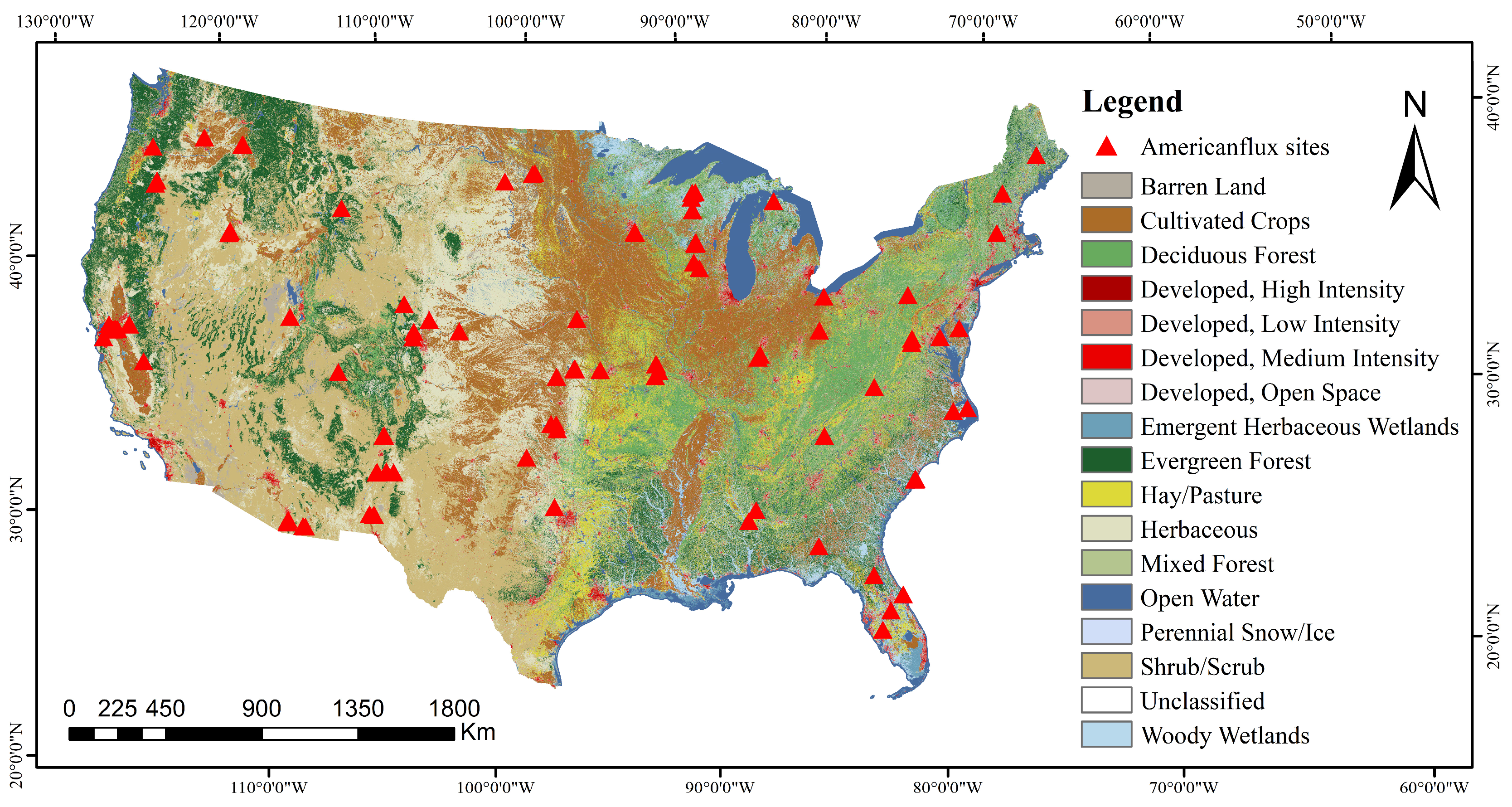
2.1. Eddy Covariance Flux Tower Data

The flux site data were obtained from the American flux network (https://ameriflux.lbl.gov/, accessed on 17 April 2024), comprising eddy covariance (EC) observations that capture exchanges of carbon, water, and energy between ecosystem surfaces and the atmosphere at high temporal frequencies [30]. GPP_VUT_NT is derived using the nighttime partitioning method and is frequently utilized as a benchmark for GPP estimates in recent research [31,32,33]. The study selected data from 2015 to 2020. To be included in the dataset, daily site observations were required to have related remote sensing data and meet acceptable quality criteria. Observations were excluded from the dataset if the value of the quality label was less than 0.75. The reference values for estimating GPP are derived from GPP_VUT_NT_REF. To align the temporal resolution of most GPP products, high-quality flux data were extracted every eight days using quality flags, and any data with negative GPP values were removed. The final dataset includes 13,298 site records collected from 114 sites across the United States. Data from 11,222 records across 72 sites were used for model training and validation, with the remaining data reserved for accuracy comparison with other products. Figure 1 presents detailed information on vegetation types and site distribution in the study area. We computed a Moran’s I index of 0.557 for the original site observation data, with a p-value of less than 0.01, indicating significant spatial autocorrelation among the sites, necessitating the consideration of spatial effects in further research.

2.2. Remote Sensing Data

The remote sensing data presented in

Table 1. Remote sensing products and variables in this study.

Product	Band	Temporal Resolution	Spatial Resolution	Source
GLASS	DSR	Daily	0.05°	http://www.glass.umd.edu/ (accessed on 16 April 2024)
MCD43A4	Band1 (620–670 nm)	Daily	500 m	https://lpdaac.usgs.gov/products/mcd43a4v061/ (accessed on 19 April 2024)
	Band2 (841–876 nm)
	Band3 (459–479 nm)
	Band4 (545–565 nm)
	Band5 (1230–1250 nm)
	Band6 (1628–1652 nm)
	Band7 (2105–2155 nm)
MOD11A1	Band31 (10.780–11.280 μm)	Daily	1 km	https://lpdaac.usgs.gov/products/mod11a1v061/ (accessed on 19 April 2024)
	Band32 (11.770–12.270 μm)
MODOCGA	Band11 (526–536 nm)	Daily	1 km	https://lpdaac.usgs.gov/products/modocgav006/ (accessed on 19 April 2024)
MOD13Q1	EVI	16 days	250 m	https://lpdaac.usgs.gov/products/mod13q1v061/ (accessed on 19 April 2024)

were utilized during the construction of the GPP estimation model. Among these, the GLASS downward shortwave radiation data played an important role in furnishing information concerning radiant energy, which serves as the primary energy input for photosynthesis [34]. The GLASS data were processed using information from multiple sensors and satellite platforms, including but not limited to various multispectral and hyperspectral sensors like MODIS, AVHRR (Advanced Very High-Resolution Radiometer), and MERIS (Medium-Resolution Imaging Spectrometer). MCD43A4 is a Nadir Bidirectional Reflectance Distribution Function–Adjusted Reflectance dataset and contains MODIS bands from 1 to 7. The MOD11A1 dataset contributes to surface temperature. Band 11 of the MODOCGA dataset can track the changes in xanthophyll during the photosynthesis process and serves as an input for the photochemical reflectance index [35]. Additionally, the MOD13Q1 dataset provides the Enhanced Vegetation Index (EVI), which reflects vegetation growth vigor. These data cover important factors affecting vegetation photosynthesis, collectively offering comprehensive information on vegetation growth and GPP variations.

We associated each record from the site dataset with the corresponding remote sensing data. Every satellite dataset underwent a quality label filtration process and was later resampled to a 1 km resolution using the GEE, with the exception of the GLASS dataset. In addition to the central pixel of flux sites, the surrounding 24 pixels (approximately 5 km × 5 km) were also considered for contrast with other GPP products that have coarser spatial resolutions.

2.3. Comparative Analysis of GPP Products

MOD17 and GOSIF were chosen to assess the model’s effectiveness. The spatial resolutions of the MOD17 and GOSIF are 500 m and 0.05°, respectively, with both having a temporal resolution of eight days. MOD17 (https://lpdaac.usgs.gov/products/mod17a2hv061/, accessed on 22 April 2024) utilizes the LUE (light use efficiency) model, which integrates data such as PAR (photosynthetically active radiation), vegetation indices, temperature, and vapor pressure deficit to describe the photosynthesis process [36]. When calculating GPP, the LUE model combines these input data and uses the vegetation’s light use efficiency to calculate the amount of carbon fixed by photosynthesis [37], as shown in Equation (1).

$$\mathrm{G}\mathrm{P}\mathrm{P}=\mathrm{P}\mathrm{A}\mathrm{R}\times \mathrm{f}\mathrm{P}\mathrm{A}\mathrm{R}\times \in$$

(1)

where PAR is photosynthetically active radiation, FPAR is the fraction of PAR absorbed by vegetation, and ε is the light use efficiency, representing the efficiency with which plants convert absorbed PAR into organic matter.

GOSIF (http://globalecology.unh.edu/data/, accessed on 22 April 2024), on the other hand, relies on OCO-2 satellite data and estimates GPP by measuring the byproduct of photosynthesis [38]. SIF is a measure of plant fluorescence emitted during photosynthesis and is correlated with the intensity of this process. GOSIF combines EVI, land cover type, and meteorological data, using the Cubist regression tree model (based on Quinlan’s M5 model tree) to create rule-based predictive models, where each rule is associated with a multivariate linear regression model, to calculate the GPP of surface vegetation [39]. Both the MODIS GPP and GOSIF GPP products have been subject to scrutiny in previous research efforts [40,41,42,43,44].

3. Methodology

The steps of this study are as follows: (1) assessing the Pearson correlation coefficients and feature importance of the initial variables and screening out the variables closely related to GPP as the model variables; (2) confirming the spatial autocorrelation effect on GPP estimation at the study area sites, constructing the spatial weights matrix, extracting the eigenvectors, and incorporating spatial factors into the input variables; (3) constructing the GPP estimation model founded on a spatial autocorrelation light gradient boosting machine model (SA-LGBM) and validating its accuracy; (4) comparing the performance of various GPP products at different temporal scales, in addition to the applicability of models across different spatial and temporal scales (Figure 2).

3.1. Variables Selection for GPP Estimation Model

In this study, 13 variables associated with vegetation GPP were selected based on photosynthesis mechanisms, including Band1–7, DSR, EVI, Band11, Month, Band31, and Band32. Variable selection was performed prior to model construction. A Pearson correlation analysis, a widely used method, was employed to examine the correlation between variables and GPP. The Pearson correlation coefficient is defined in Equation (2). Usually, a significance level of 5% is employed, indicating that if the p-value falls below 0.05, the null hypothesis is rejected at a 95% confidence level. Consequently, variables with a Pearson correlation coefficient p-value > 0.05 were excluded due to uncertain reliability. For significant variables, those with an absolute Pearson correlation coefficient exceeding 0.1 were considered to have a substantial relationship [45]:

$$r=\frac{{\sum }_{i=1}^n\left(x_i-\overline{x}\right)\left(y_i-\overline{y}\right)}{\sqrt{{\sum }_{i=1}^n{\left(x_i-\overline{x}\right)}^2{\sum }_{i=1}^n{\left(y_i-\overline{y}\right)}^2}}$$

(2)

where $x_i$ and $y_i$ represent the values of an individual variable and GPP, respectively, while $\overline{x}$ and $\overline{y}$ represent the mean values of each variable and GPP.

A feature importance evaluation was performed. Feature importance is quantified by measuring the reduction in model performance when predictions are made on a dataset where the values of a particular feature have been randomly shuffled across rows. For instance, a score of 0.01 implies that predictive accuracy decreased by 0.01 when the feature was shuffled. Features with higher scores are deemed more critical for the model’s performance. Conversely, a negative score indicates that a feature could have an adverse impact on the model and that eliminating it may enhance predictive performance.

3.2. Extraction of Spatial Factors at American Flux Sites

In accordance with the first law of geography, spatial autocorrelation may influence the distribution of GPP, where similarities among different locations can lead to data correlations. When modeling based on site observation data, it is essential to employ a simple yet effective approach to account for the spatial effects of variables, thereby obtaining more accurate and stable results. To mitigate spatial autocorrelation in the spatial distribution of GPP, we adopted a method for extracting spatial factors. The ESF method derives these spatial factors by computing and filtering the spatial eigenvectors of the spatial weights matrix. Incorporating spatial eigenvectors effectively addresses the influence of spatial autocorrelation.

The extraction of spatial factors comprises the subsequent four stages:

(1)

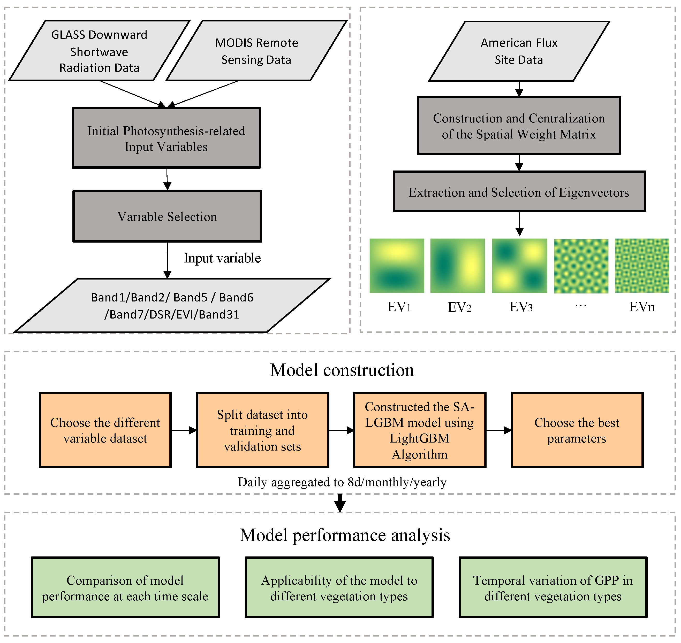
Building the spatial weights matrix: The initial phase entails constructing the spatial weights matrix by leveraging the spatial connections inherent in the American flux site data. This matrix is created using the Spatial Covariance Function for the coordinates of the monitoring sites. The Gaussian model assumes that the weights decay with distance in the form of a Gaussian distribution. Equation (3) represents the Gaussian model:

$${\mathrm{W}}_{i,j}=\exp \left(-{\left(\frac{{\mathrm{d}}_{i,j}}{\mathrm{r}}\right)}^2\right)$$

(3)

where $i$ and $j$ denote location points $i$ and $j$, respectively; ${\mathrm{W}}_{i,j}$ denotes the neighborhood weight between location points $i$ and $j$; and $\mathrm{r}$ denotes the furthest distance in the smallest spanning tree across all locations.

From the formula, it can be found that ${\mathrm{W}}_{i,j}$ = ${\mathrm{W}}_{j,i}$; if there are n monitoring stations, the final result is an $\mathrm{n}$ × $\mathrm{n}$ matrix, the elements on the diagonal are 0, and the remainder of the elements are the results calculated via the above equation and are symmetric matrices.

(2)

Centralizing the spatial weights matrix: The spatial weights matrix ${\mathrm{W}}_0$ is centralized employing the subsequent approach:

$$\mathrm{C}=\left(\mathrm{I}-\frac{11^{\mathrm{T}}}{\mathrm{n}}\right){\mathrm{W}}_0\left(\mathrm{I}-\frac{11^{\mathrm{T}}}{\mathrm{n}}\right)$$

(4)

where $\mathrm{I}$ is an n-dimensional unit matrix, $11^{\mathrm{T}}$ is an n × n matrix with all elements within the matrix equal to 1, and $\mathrm{n}$ is the number of flux sites.

(3)

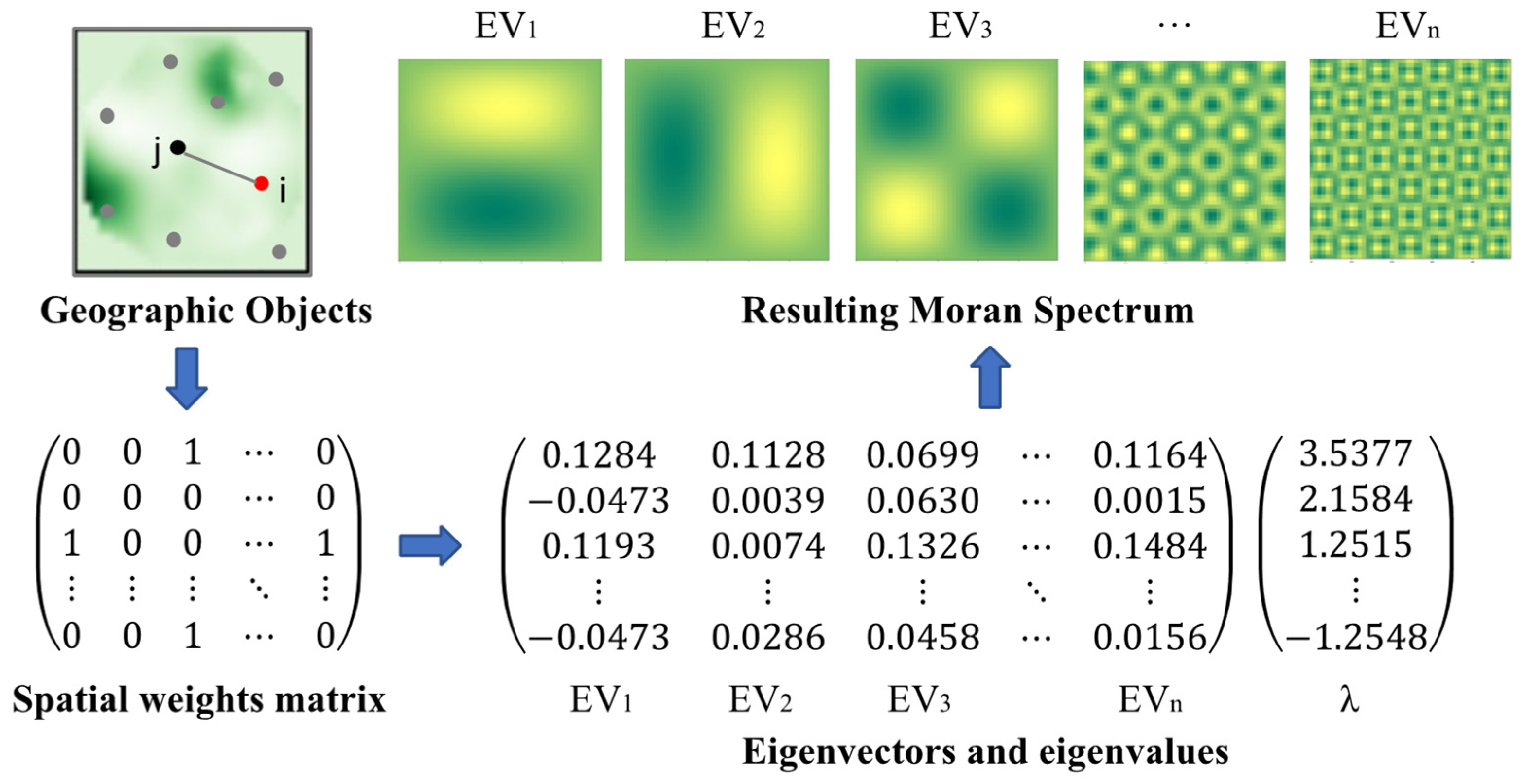
Extraction of eigenvalues and eigenvectors: We perform eigen decomposition on the centralized matrix, yielding eigenvalues and eigenvectors, while ensuring they satisfy the conditions of Equation (5):

$$\mathrm{D}\mathrm{e}\mathrm{t}\left(\mathrm{C}-\mathsf{\lambda }\mathrm{I}\right)=0$$

(5)

where Det represents the matrix determinant operator, λ is the eigenvalue, and I is the identity matrix. Each eigenvector obtained through this process represents a specific spatial pattern. The relationship between the spatial weights matrix and its corresponding eigenvalues and eigenvectors is illustrated in Figure 3.

(4)

Eigenvector screening: An initial screening of eigenvectors is carried out using a threshold of 0.25. ${\mathrm{E}\mathrm{V}}_{\mathrm{n}}$ must meet the following criteria with respect to their corresponding eigenvalues ${\mathsf{\lambda }}_{\mathrm{n}}$: 1. ${\mathsf{\lambda }}_{\mathrm{n}}$ > 0; 2. The ratio of the eigenvalue to the maximum eigenvalue in the set should exceed 0.25. The screened eigenvectors can reflect varying degrees of spatial clustering, with larger eigenvalues indicating stronger clustering, which are subsequently integrated with the model as independent variables.

3.3. Construction of the GPP Estimation Model

By exploring a range of machine learning algorithms, we investigated the complex interplay between input variables and GPP to develop the estimation model. These algorithms include LightGBM [45], CatBoost [46], PyTorch neural network model [47], ExtraTrees [48], XGBoost [49], and Random Forest [50], all of which are well-established tools for GPP estimation, each with its own set of strengths and characteristics. We leveraged AutoGluon’s automated feature engineering and hyperparameter tuning capabilities to split the dataset into training and validation sets, optimizing the parameter settings for each model to achieve the best possible performance. A total of 11,222 records from 72 sites were used for model training and validation. The training set and validation set were divided into an 80:20 ratio, and ten-fold cross-validation was employed for training. The final estimates were derived from the mean outcomes obtained through the ten-fold cross-validation procedure. The remaining data were reserved for accuracy testing and comparison. Following a series of experiments and evaluations, we identified LightGBM as the top-performing method. LightGBM utilizes gradient boosting methodologies, which entail sequentially training a series of weak learners, usually decision trees, and subsequently aggregating them to form a robust model. Furthermore, as depicted in Figure 4, we incorporated spatial factors into our modeling approach and developed a spatial autocorrelation LightGBM-based model (SA-LGBM) to enhance GPP estimation. This model fully accounts for the similarities and spatial correlations between different locations, allowing for a better capture of GPP’s spatial distribution.

3.4. Accuracy Assessment

3.4.1. Model Evaluation Indicators

To evaluate the efficacy of models and the precision of their alignment with actual GPP, the $R^2$ and root mean square error (RMSE) are employed as assessment criteria. $R^2$ indicates the proportion of the dependent variable modeled explained by the model, while RMSE quantifies the difference between the observed values and the actual values of the dependent variable. They are shown in Equations (6) and (7):

$$R^2=1-\frac{{\sum }_{i=1}^n{\left(y_i-\widehat{y_i}\right)}^2}{{\sum }_{i=1}^n{\left(y_i-\overline{y}\right)}^2}$$

(6)

where $y_i$ represents the actual GPP, $\widehat{y_i}$ is the estimated GPP, and $\overline{y}$ is the average GPP.

$$RMSE=\sqrt{\frac{1}{n}{\displaystyle \sum _{i=1}^n}{\left(y_i-\widehat{y_i}\right)}^2}$$

(7)

where $n$ denotes the total number of samples, $y_i$ denotes the actual GPP, and $\widehat{y_i}$ denotes the estimated GPP.

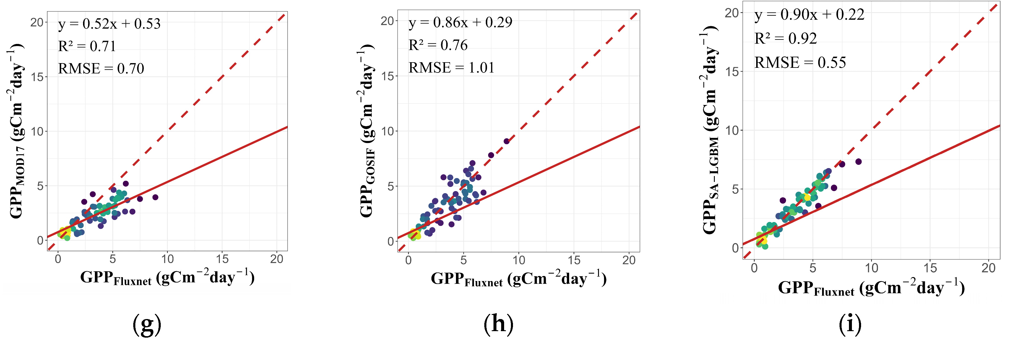
3.4.2. Accuracy Comparison

A comprehensive accuracy evaluation of the estimation results of the SA-LGBM model is conducted in our study using eddy covariance flux tower observations and two GPP products, MOD17 and GOSIF. We aggregated the original results obtained at a 500 m resolution from MOD17 and a 1 km resolution from SA-LGBM to a 5 km resolution for further analysis. This was carried out to accommodate the relatively limited spatial resolution of existing GPP products. In the experimental comparison, we fully considered the effect of the time scale and performed the comparative analysis at three different scales, from an 8-day scale, to monthly, to annual. Such multi-scale comparisons help us obtain a comprehensive awareness of the performance of the SA-LGBM model, while also capturing multiple aspects of its spatiotemporal generalization ability. We adopted the RMSE and $R^2$ as metrics for quantitative analysis, which can effectively measure the error between model estimates and actual observed data, as well as the degree of fit.

3.4.3. Assessment of the Spatial Effects

When spatial data without accounting for spatial effects are employed in a data-driven model, residual spatial autocorrelation may persist [51,52,53]. In an ideal scenario, the goal is to minimize or completely eliminate spatial autocorrelation in residuals. This ensures that the model’s performance remains consistent across geographic regions, minimizing gross overestimates or underestimates. The EV extracted from the spatial weights matrix is pivotal in connecting geographic entities in space. Subsequently, the EV is incorporated into the SA-LGBM as a control variable, effectively identifying and separating spatial dependencies from GPP. When making predictions, we perform spatial interpolation on these sets of eigenvectors based on the extent of the raster data and use them as inputs to the model. To measure distributions and spatial autocorrelation in the residuals, Moran’s I metric was used to measure spatial autocorrelation.

4. Results

4.1. Variable Selection for GPP Estimation Model

The Pearson correlation coefficients between all variables related to photosynthesis and GPP are shown in Figure 5. Darker colors indicate stronger correlations, while white pixels represent no correlation between the two variables. All displayed values passed significance tests. Only variables with a correlation greater than 0.1 with GPP were retained. Among them, Band32 and Month had a correlation of less than 0.1 with GPP. If the correlation between independent variables was greater than 0.8, only one of them was kept. Therefore, Band32, Month, Band3, and Band4 were excluded when building the model. This was carried out to avoid the impact of multicollinearity between variables and to reduce the complexity of the model.

The feature importance scores for each variable are shown in

Table 2. Feature importance of variables and p-values.

Variables	Importance	Stddev	p-Value
Band2	1.52	0.04	7.45 × 10−9
Band1	1.31	0.02	2.81 × 10−8
DSR	1.18	0.05	3.70 × 10−7
EVI	0.96	0.02	1.21 × 10−8
Band7	0.79	0.01	4.28 × 10−8
Band5	0.59	0.02	5.82 × 10−7
Band6	0.31	0.01	4.75 × 10−7
Band31	0.18	0.01	5.47 × 10−6
Band11	0.01	0.00	0.000283

. Stddev represents the standard deviation of the feature importance scores, measuring the variability in importance scores. The last column shows the p-value used for the statistical T-test, where the null hypothesis assumes the variable’s importance score is 0 and the alternative hypothesis assumes the importance score is greater than 0. Lower p-values indicate strong evidence against the null hypothesis, indicating that the importance scores of these variables are significantly greater than 0 and are valuable for the predictive model. It can be observed that Band2, Band1, DSR, and EVI are relatively important for the predictive model. The feature importance of Band11 is very low, with a significant inflection point, and there is a considerable amount of missing data. Considering both the complexity of the model and data integrity, Band11 was excluded when building the model.

4.2. Model Fitting and Validation

This study involved a contrast of the accuracy of commonly used machine learning methods in GPP estimation, including CatBoost, Random Forest, XGBoost, PyTorch Neural Net model, ExtraTrees, and LightGBM. As shown in

Table 3. Accuracy comparison of different machine learning methods incorporating spatial factors.

Model	Test Set (Without Spatial Factors)		Test Set (With Spatial Factors)
	${\mathit{R}}^2$	RMSE	${\mathit{R}}^2$	RMSE
PyTorch Neural Net model	0.80	1.70	0.86	1.46
XGBoost	0.80	1.69	0.86	1.44
CatBoost	0.81	1.66	0.88	1.35
ExtraTrees	0.80	1.69	0.86	1.45
Random Forest	0.81	1.67	0.87	1.43
LightGBM	0.82	1.63	0.89	1.29

, LightGBM outperforms the other models without considering the spatial factors provided by the ESF method. After incorporating spatial factors, all models showed different levels of enhancement in performance. It is evident that the SA-LGBM model outperforms the others. With the inclusion of EV, we observed an 8.5% increase in $R^2$ and a 20.8% decrease in RMSE. This indicates that incorporating spatial vectors can enhance the model’s precision and the influence of spatial autocorrelation is mitigated in the model.

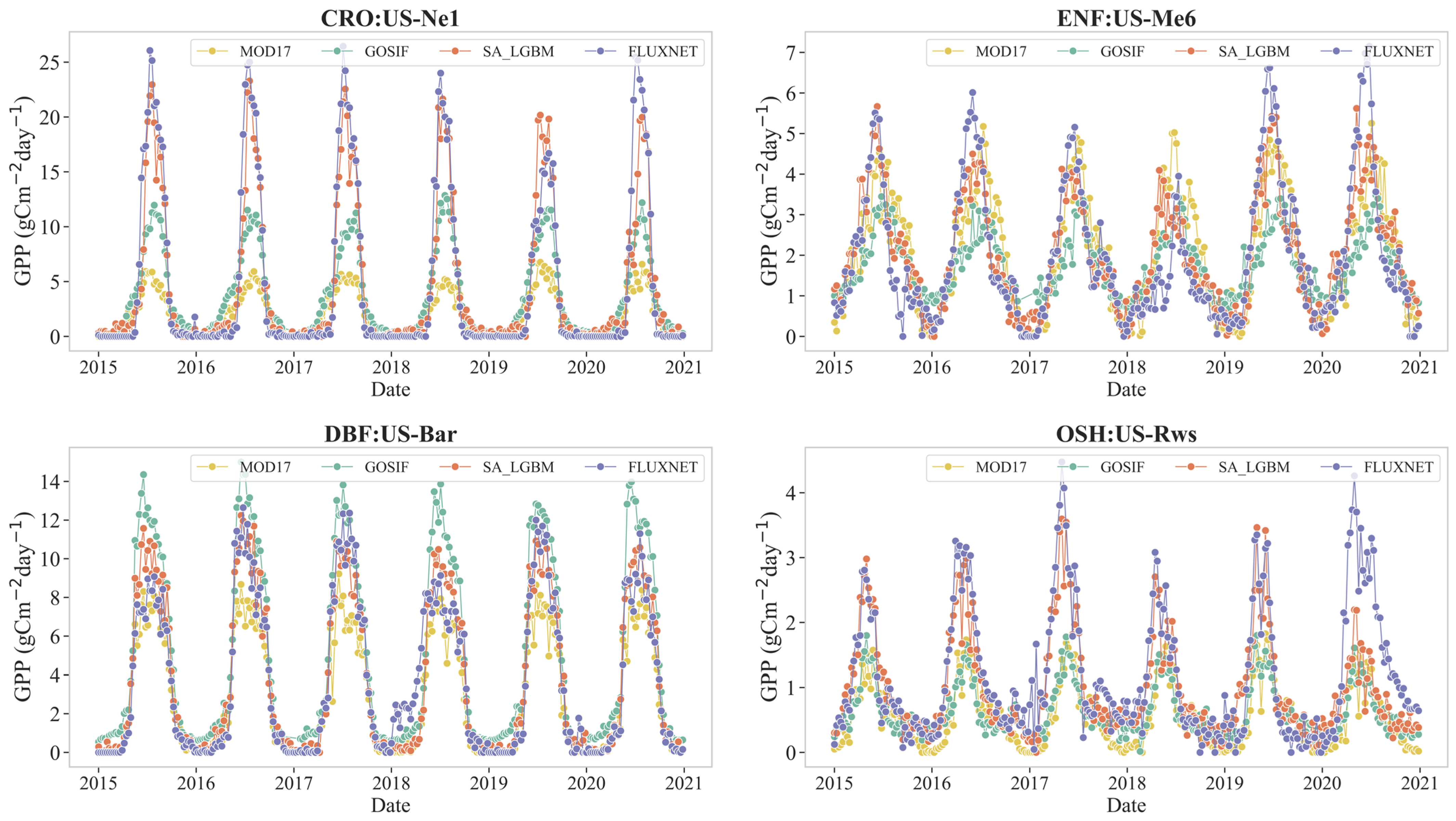
4.3. Assessment of GPP at Different Temporal Scales

A comparison of GPP estimates from the SA-LGBM model with other GPP products was conducted within a footprint near the flux sites. The overall correlation of SA-LGBM with eddy covariance flux tower data is notably higher, as illustrated in Figure 6. In all time scales, SA-LGBM exhibits superior performance, boasting higher $R^2$ and lower RMSE. Averaging over all time scales, the $R^2$ of SA-LGBM is 0.21 higher than that of MOD17 and 0.17 higher than that of GOSIF. These results imply that the SA-LGBM has the ability to not only capture daily fluctuations in GPP but also variations in GPP across seasonal and interannual timeframes. Overall, SA-LGBM partially overcomes the shortcomings of the existing model of “high observation and low estimation” and achieves better results.

4.4. Assessment of GPP in Different Vegetation Types

In the real world, vegetation is typically a mixture of different types of vegetation. Traditional GPP estimation methods require prior knowledge of the vegetation composition in the target area, which can be challenging in complex and diverse vegetation environments [54]. Six representative vegetation types were selected to assess the model’s applicability in different vegetation types, namely, grasslands (GRA), croplands (CRO), evergreen needleleaf forests (ENF), permanent wetlands (WET), deciduous broadleaf forests (DBF), and open shrublands (OSH). Figure 7 shows the R² and RMSE of different GPP products across various vegetation types. SA-LGBM performs nearly as well as or better than other GPP products across all vegetation types, except in the WET type where its performance is not as prominent. Notably, in regions with relatively low vegetation productivity, such as the OSH type, the predictive capability of all GPP products is not outstanding [40,55]. However, SA-LGBM significantly outperforms other products and demonstrates good spatial generalization capability.

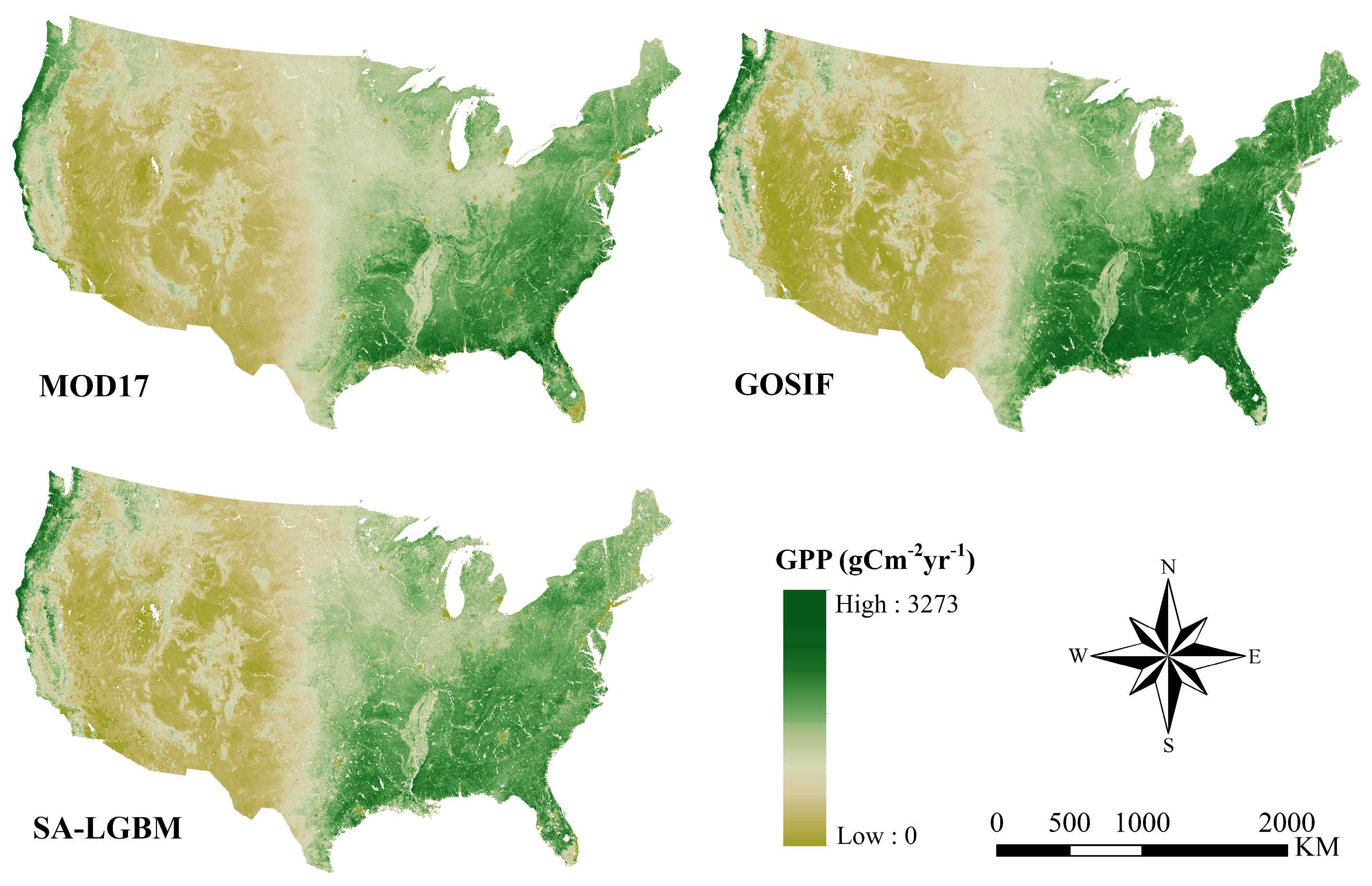
4.5. Mapping and Comparison of GPP Estimation Results

Figure 8 shows the GPP estimation results for the continental United States in 2020 using the SA-LGBM model, as well as the spatial distribution of GPP from the MOD17 and GOSIF products. It can be seen that these three products exhibit similar spatial distribution characteristics, with high GPP values primarily concentrated in densely forested areas. The highest GPP values are found in the Great Lakes region, the Appalachian Mountains, and along the Pacific coast, with values ranging from approximately 2000 to 3000 $\mathrm{g}\mathrm{C}{\mathrm{m}}^{-2}{\mathrm{y}\mathrm{r}}^{-1}$. The agricultural areas in the Midwest exhibit moderate GPP values. The arid regions in the Southwest, including Nevada, Arizona, and New Mexico, have relatively low GPP values due to limited rainfall, sparse vegetation, and restricted photosynthesis. Compared to GOSIF, MOD17 and SA-LGBM show less variability.

Figure 9 shows the residual distribution of three GPP products in 2020. Although SA-LGBM, MOD17, and GOSIF are generally consistent in GPP estimation, there are significant differences in certain regions. In many areas of the eastern United States, GOSIF estimates higher GPP values than SA-LGBM and SA-LGBM estimates higher values than MOD17. In contrast, the opposite pattern is observed in the western regions. GOSIF uses SIF data, which are directly associated with plant photosynthesis and directly reflect the activity of photosynthesis. Particularly in the densely vegetated eastern regions, GOSIF may capture higher GPP. MOD17 tends to underestimate GPP in areas with high GPP.

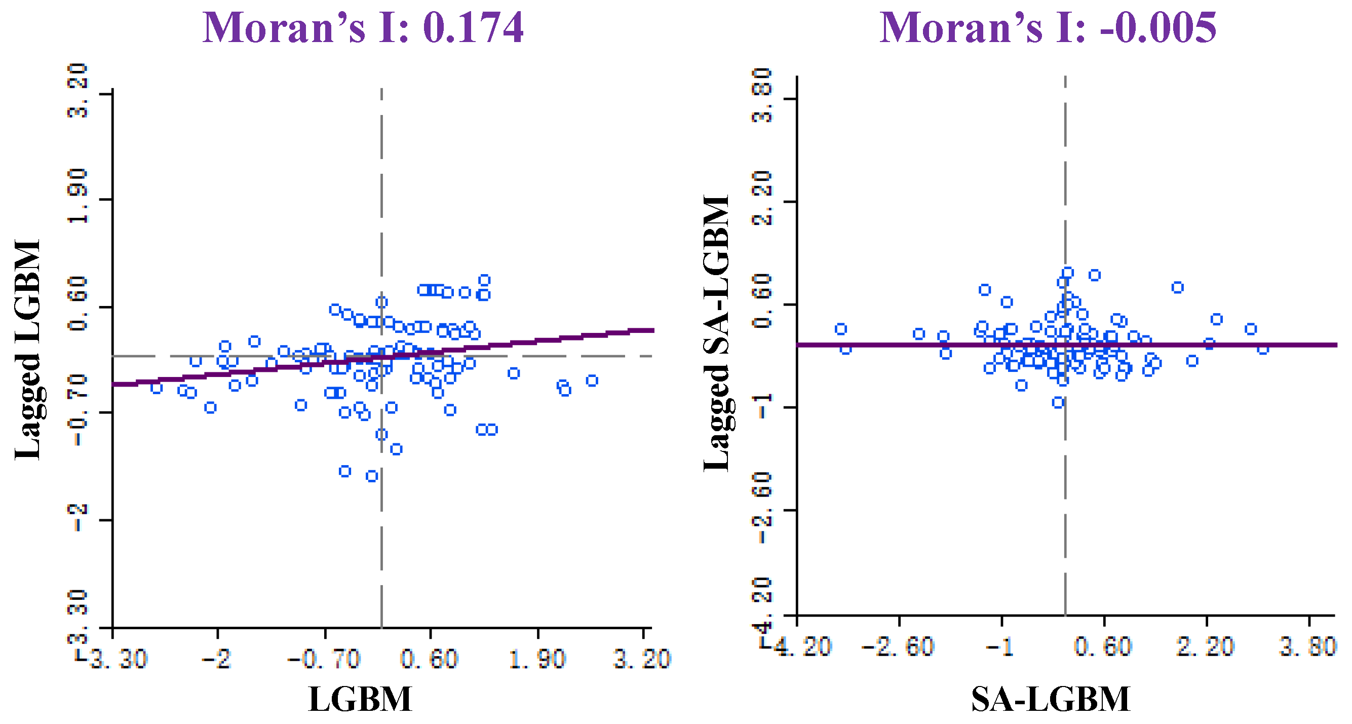
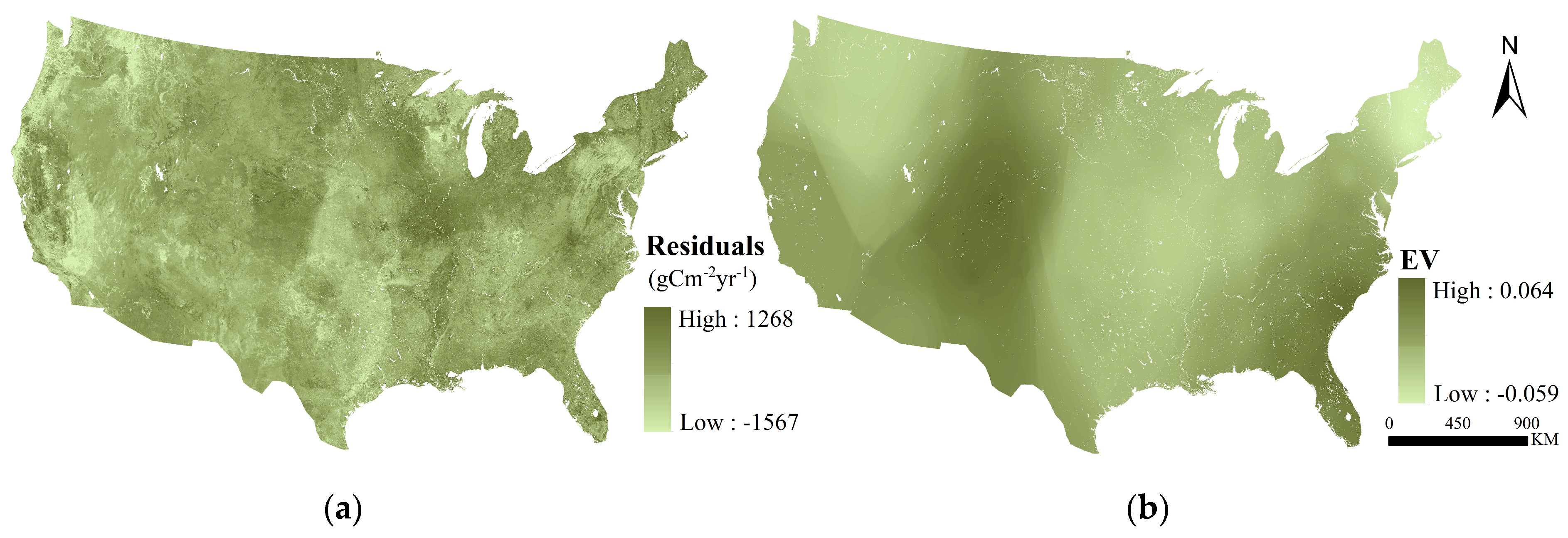
4.6. Impact Assessment of Spatial Effects

Spatial autocorrelation is taken into account in the SA-LGBM. In the real world, vegetation distribution often exhibits a certain degree of spatial correlation. SA-LGBM is capable of better capturing this correlation by introducing spatial eigenvectors, which enables a more effective understanding and quantification of the similarity between different locations. The integration of spatial autocorrelation into the model has been demonstrated to enhance the dependability and precision of the estimation outcomes [29,56].

Figure 10 introduces a variable Z, which represents the magnitude of residuals deviating from their mean value. Consequently, Z is distributed on both sides of the zero value. The vertical axis variable represents the sum of the values of neighboring features multiplied by their respective normalized weight values, reflecting the overall level of neighboring features. It is evident that points falling in the first quadrant, whether they represent the element or its neighboring elements, exhibit relatively large residuals compared to the mean, indicating a high–high spatial pattern. The second quadrant signifies a spatial pattern where regions with high residual values are surrounded by regions with low values. To measure spatial autocorrelation in residuals, Moran’s I index was employed. Prior to the inclusion of EV, Moran’s I for residuals in the LGBM model was high and significant, indicating a certain degree of spatial correlation among neighboring residual values. This may suggest that the model failed to fully capture spatial patterns, resulting in a non-random and statistically significant spatial distribution of residuals. After incorporating EV, Moran’s I of residuals in the SA-LGBM model became low and insignificant, indicating that spatial autocorrelation had been removed, and the residuals can be considered as random errors within the SA-LGBM model.

Utilizing the first law of geography, we constructed a spatial weights matrix to depict the interrelations among American flux sites, and subsequently generate and extract EV. By subtracting the GPP in the LGBM model from the GPP in the SA-LGBM model, the impact of EV within the model can be discerned through the distribution of GPP residuals [57]. Figure 11 depicts the spatial distribution of residuals for both the LGBM and SA-LGBM models, along with the spatial distribution of EV. Notably, the distribution of GPP residuals exhibits a similar trend to the changes in EV. There exists a strong consistency between the distribution of GPP residuals and the spatial distribution of EV, suggesting that EV can be considered as a complementary variable for capturing the spatial effects in GPP.

5. Discussion

5.1. Advantages of SA-LGBM

SA-LGBM significantly enhances the precision of GPP estimation. By combining the ESF method, sophisticated nonlinear model design, and an ample training dataset, SA-LGBM effectively reduces estimation errors, providing more precise results for remote sensing-based GPP estimation. The performance of common machine learning methods in GPP estimation is compared in our experiment, revealing that LGBM outperformed these other methods when not considering the spatial effects. Building upon this, we improved the model by incorporating spatial factors, resulting in the superior performance of the SA-LGBM model. The inclusion of EV led to an 8.5% increase in $R^2$ and a 20.8% reduction in RMSE. This improvement was achieved through the synergistic combination of the ESF method, the nonlinear model structure, and the comprehensive training dataset, significantly reducing estimation errors and yielding more accurate remote sensing GPP estimates. Furthermore, within the footprint range near the flux tower sites, we compared GPP estimates produced by the SA-LGBM model with other GPP products. SA-LGBM demonstrated a notably higher overall correlation with flux data. Across all time scales, SA-LGBM consistently exhibited outstanding performance. Compared to MOD17 and GOSIF, SA-LGBM achieved a 0.21 and 0.17 average increase in $R^2$ across different time scales. In conclusion, SA-LGBM has the capability to provide more accurate results across various time scales. In addition, the discrepancy in estimating flux tower GPP by MOD17 and GOSIF, resulting in underestimation, has been extensively documented in the literature [40,58,59], and SA-LGBM overcomes the underestimation of the existing GPP products to a certain extent and achieves better results.

SA-LGBM, through the ESF method, effectively and succinctly extracted the inherent spatial autocorrelation between GPP flux sites, resulting in more accurate GPP estimates. In contrast, the residuals of LGBM without spatial factors exhibit statistically significant spatial autocorrelation, indicating the existence of spatial dependencies within the data that LGBM failed to capture. Ignoring these dependencies can lead to biased and inefficient estimates. By considering the intrinsic spatial organization within the dataset, SA-LGBM makes the model residuals more random and less spatially structured, which is a key assumption in many statistical analyses [29,60,61].These findings align with our expectations that incorporating spatial information should help capture spatial autocorrelation and improve accuracy, thereby reinforcing the results of previous related research [62,63,64].

SA-LGBM is entirely based on remote sensing observation data, without considering plant functional types, multi-source data, or inherent parameters. Compared to other models that use precipitation and vapor pressure deficit data [65,66,67], SA-LGBM can reduce the uncertainties associated with interpolated meteorological data, and its input data have higher availability.

5.2. Ability of the Three GPP Products to Capture GPP Variations

To further evaluate the capability of SA-LGBM and other GPP products in capturing GPP variations and their suitability across different vegetation types, we selected representative locations for six distinct vegetation types, which are grasslands (GRA), croplands (CRO), evergreen needleleaf forests (ENF), permanent wetlands (WET), deciduous broadleaf forests (DBF), and open shrublands (OSH). We conducted a quantitative assessment of their seasonal changes from 2015 to 2020, as depicted in Figure 12. We ensured that each site possessed quality samples corresponding to the relevant vegetation type. All three products effectively depict the seasonal fluctuations of GPP across sites featuring diverse vegetation types, demonstrating uniformity in general patterns, notably in the timing of GPP peak occurrences and overall variability trends. GPP generally peaks in summer each year and approaches zero in winter. It can be observed that MOD17 exhibits a significant underestimation for sites with high GPP values, such as CRO and GRA types. This is consistent with previous research findings [58,59]. We found that SA-LGBM has the highest fitting degree with flux site data, effectively capturing vegetation signals across a wide range of GPP. SA-LGBM largely overcomes the underestimation issue of existing GPP products in areas with high vegetation signals [68]. The ability of the three products to detect GPP changes in sparse vegetation is unstable and exhibits significant fluctuations. Overall, SA-LGBM exhibits good adaptability and can capture variations across different geographic regions and vegetation types. Especially in areas with complex vegetation types, the SA-LGBM method accurately reflects subtle changes in GPP, providing more reliable estimation results.

5.3. Limitations and Future Enhancement

The precision of GPP estimation with SA-LGBM could be impacted by the composition of training data and the design of model variables. While we have screened flux sites for model training, data from regions with comparatively modest vegetation productivity are scarce. This limitation may result in reduced applicability of SA-LGBM in such areas, as observed in the less stable OSH results shown in Figure 10. Enhanced generalizations of SA-LGBM could be achieved by incorporating more flux tower observations encompassing a wider rang of vegetation types. This study considers the impact of spatial autocorrelation on GPP estimation models. Furthermore, it is essential to investigate the influence of spatial heterogeneity on modeling. Recent research has indicated the presence of additional information related to GPP in SIF data [69,70,71]. Whether the use of SIF can lead to improved GPP estimation beyond reflectance-based approaches needs to be confirmed.

6. Conclusions

This study introduces a novel GPP remote sensing estimation model, SA-LGBM, which incorporates considerations for spatial autocorrelation. We found that incorporating spatial factors led to varying degrees of improvement in model accuracy for different machine learning methods. Specifically, the SA-LGBM model exhibited an 8.5% increase in $R^2$ and a 20.8% decrease in RMSE after incorporating spatial factors. Compared to LGBM, SA-LGBM reduces the spatial autocorrelation of prediction residuals. The residuals of the model are more random, with less spatial structure. EV can be considered as a variable capturing the spatial distribution characteristics of GPP, which has a positive effect on the model. Furthermore, the SA-LGBM model showed relatively favorable results compared to existing GPP products. Compared to MOD17 and GOSIF, SA-LGBM achieved an average increase in $R^2$ of 0.21 and 0.17 across different time scales. SA-LGBM demonstrates good applicability across different vegetation types and can effectively capture the spatiotemporal variation characteristics of GPP. These findings align with our expectations, indicating that incorporating spatial information helps capture spatial autocorrelation and improves the accuracy of GPP estimation.

References

1. Zhang, F.; Chen, J.M.; Chen, J.; Gough, C.M.; Martin, T.A.; Dragoni, D. Evaluating Spatial and Temporal Patterns of MODIS GPP over the Conterminous U.S. against Flux Measurements and a Process Model. Remote Sens. Environ. 2012, 124, 717–729. [Google Scholar] [CrossRef]
2. Friedlingstein, P.; Jones, M.W.; O’Sullivan, M.; Andrew, R.M.; Hauck, J.; Peters, G.P.; Peters, W.; Pongratz, J.; Sitch, S.; Le Quéré, C.; et al. Global Carbon Budget 2019. Earth Syst. Sci. Data 2019, 11, 1783–1838. [Google Scholar] [CrossRef]
3. Dunkl, I.; Lovenduski, N.; Collalti, A.; Arora, V.K.; Ilyina, T.; Brovkin, V. Gross Primary Productivity and the Predictability of CO2: More Uncertainty in What We Predict than How Well We Predict It. Biogeosciences 2023, 20, 3523–3538. [Google Scholar] [CrossRef]
4. Zhang, Z.; Li, X.; Ju, W.; Zhou, Y.; Cheng, X. Improved Estimation of Global Gross Primary Productivity during 1981–2020 Using the Optimized P Model. Sci. Total Environ. 2022, 838, 156172. [Google Scholar] [CrossRef] [PubMed]
5. Liao, Z.; Zhou, B.; Zhu, J.; Jia, H.; Fei, X. A Critical Review of Methods, Principles and Progress for Estimating the Gross Primary Productivity of Terrestrial Ecosystems. Front. Environ. Sci. 2023, 11, 464. [Google Scholar] [CrossRef]
6. Zhang, Y.; Hu, Z.; Wang, J.; Gao, X.; Yang, C.; Yang, F.; Wu, G. Temporal Upscaling of MODIS Instantaneous FAPAR Improves Forest Gross Primary Productivity (GPP) Simulation. Int. J. Appl. Earth Obs. Geoinf. 2023, 121, 103360. [Google Scholar] [CrossRef]
7. Sun, Z.; Wang, X.; Zhang, X.; Tani, H.; Guo, E.; Yin, S.; Zhang, T. Evaluating and Comparing Remote Sensing Terrestrial GPP Models for Their Response to Climate Variability and CO2 Trends. Sci. Total Environ. 2019, 668, 696–713. [Google Scholar] [CrossRef] [PubMed]
8. Yuan, W.; Cai, W.; Liu, D.; Dong, W. Satellite-Based Vegetation Production Models of Terrestrial Ecosystem: An Overview. Adv. Earth Sci. 2014, 29, 541. [Google Scholar] [CrossRef]
9. Wen, J.; Köhler, P.; Duveiller, G.; Parazoo, N.C.; Magney, T.S.; Hooker, G.; Yu, L.; Chang, C.Y.; Sun, Y. A Framework for Harmonizing Multiple Satellite Instruments to Generate a Long-Term Global High Spatial-Resolution Solar-Induced Chlorophyll Fluorescence (SIF). Remote Sens. Environ. 2020, 239, 111644. [Google Scholar] [CrossRef]
10. Running, S.W.; Hunt, E.R. 8—Generalization of a Forest Ecosystem Process Model for Other Biomes, BIOME-BGC, and an Application for Global-Scale Models. In Scaling Physiological Processes; Ehleringer, J.R., Field, C.B., Eds.; Physiological Ecology; Academic Press: San Diego, CA, USA, 1993; pp. 141–158. ISBN 978-0-12-233440-5. [Google Scholar]
11. Running, S.W.; Coughlan, J.C. A General Model of Forest Ecosystem Processes for Regional Applications I. Hydrologic Balance, Canopy Gas Exchange and Primary Production Processes. Ecol. Model. 1988, 42, 125–154. [Google Scholar] [CrossRef]
12. Monteith, J.L. Solar Radiation and Productivity in Tropical Ecosystems. J. Appl. Ecol. 1972, 9, 747–766. [Google Scholar] [CrossRef]
13. Lieth, H. Modeling the Primary Productivity of the World. In Primary Productivity of the Biosphere; Lieth, H., Whittaker, R.H., Eds.; Springer: Berlin/Heidelberg, Germany, 1975; pp. 237–263. ISBN 978-3-642-80913-2. [Google Scholar]
14. Lieth, H.; Whittaker, R.H. Primary Productivity of the Biosphere; Springer Science & Business Media: Berlin/Heidelberg, Germany, 2012; Volume 14, ISBN 3-642-80913-8. [Google Scholar]
15. Chen, Y.; Gu, H.; Wang, M.; Gu, Q.; Ding, Z.; Ma, M.; Liu, R.; Tang, X. Contrasting Performance of the Remotely-Derived GPP Products over Different Climate Zones across China. Remote Sens. 2019, 11, 1855. [Google Scholar] [CrossRef]
16. Field, C.B.; Randerson, J.T.; Malmström, C.M. Global Net Primary Production: Combining Ecology and Remote Sensing. Remote Sens. Environ. 1995, 51, 74–88. [Google Scholar] [CrossRef]
17. Lv, Y.; Chi, H.; Shi, P.; Huang, D.; Gan, J.; Li, Y.; Gao, X.; Han, Y.; Chang, C.; Wan, J.; et al. Phenology-Based Maximum Light Use Efficiency for Modeling Gross Primary Production across Typical Terrestrial Ecosystems. Remote Sens. 2023, 15, 4002. [Google Scholar] [CrossRef]
18. Running, S.W.; Thornton, P.E.; Nemani, R.; Glassy, J.M. Global Terrestrial Gross and Net Primary Productivity from the Earth Observing System. In Methods in Ecosystem Science; Sala, O.E., Jackson, R.B., Mooney, H.A., Howarth, R.W., Eds.; Springer: New York, NY, USA, 2000; pp. 44–57. ISBN 978-1-4612-1224-9. [Google Scholar]
19. Xu, H.; Zhang, Z.; Wu, X.; Wan, J. Light Use Efficiency Models Incorporating Diffuse Radiation Impacts for Simulating Terrestrial Ecosystem Gross Primary Productivity: A Global Comparison. Agric. For. Meteorol. 2023, 332, 109376. [Google Scholar] [CrossRef]
20. Zhang, Z.; Xin, Q.; Li, W. Machine Learning-Based Modeling of Vegetation Leaf Area Index and Gross Primary Productivity Across North America and Comparison with a Process-Based Model. J. Adv. Model. Earth Syst. 2021, 13, e2021MS002802. [Google Scholar] [CrossRef]
21. Yu, T.; Zhang, Q.; Sun, R. Comparison of Machine Learning Methods to Up-Scale Gross Primary Production. Remote Sens. 2021, 13, 2448. [Google Scholar] [CrossRef]
22. Joiner, J.; Yoshida, Y. Satellite-Based Reflectances Capture Large Fraction of Variability in Global Gross Primary Production (GPP) at Weekly Time Scales. Agric. For. Meteorol. 2020, 291, 108092. [Google Scholar] [CrossRef]
23. Reichstein, M.; Camps-Valls, G.; Stevens, B.; Jung, M.; Denzler, J.; Carvalhais, N. Prabhat Deep Learning and Process Understanding for Data-Driven Earth System Science. Nature 2019, 566, 195–204. [Google Scholar] [CrossRef]
24. Griffith, D.A. Important Considerations about Space-Time Data: Modeling, Scrutiny, and Ratification. Trans. GIS 2021, 25, 291–310. [Google Scholar] [CrossRef]
25. Griffith, D.; Chun, Y.; Li, B. Spatial Regression Analysis Using Eigenvector Spatial Filtering; Academic Press: Cambridge, MA, USA, 2019; ISBN 978-0-12-815692-6. [Google Scholar]
26. Islam, M.D.; Li, B.; Lee, C.; Wang, X. Incorporating Spatial Information in Machine Learning: The Moran Eigenvector Spatial Filter Approach. Trans. GIS 2022, 26, 902–922. [Google Scholar] [CrossRef]
27. Brunsdon, C.; Fotheringham, S.; Charlton, M. Geographically Weighted Regression. J. R. Stat. Soc. Ser. D (Stat.) 1998, 47, 431–443. [Google Scholar] [CrossRef]
28. Murakami, D.; Griffith, D.A. Random Effects Specifications in Eigenvector Spatial Filtering: A Simulation Study. J. Geogr. Syst. 2015, 17, 311–331. [Google Scholar] [CrossRef]
29. Liu, X.; Kounadi, O.; Zurita-Milla, R. Incorporating Spatial Autocorrelation in Machine Learning Models Using Spatial Lag and Eigenvector Spatial Filtering Features. ISPRS Int. J. Geo-Inf. 2022, 11, 242. [Google Scholar] [CrossRef]
30. Baldocchi, D.; Falge, E.; Gu, L.; Olson, R.; Hollinger, D.; Running, S.; Anthoni, P.; Bernhofer, C.; Davis, K.; Evans, R.; et al. FLUXNET: A New Tool to Study the Temporal and Spatial Variability of Ecosystem-Scale Carbon Dioxide, Water Vapor, and Energy Flux Densities. Bull. Am. Meteorol. Soc. 2001, 82, 2415–2434. [Google Scholar] [CrossRef]
31. Tramontana, G.; Jung, M.; Schwalm, C.R.; Ichii, K.; Camps-Valls, G.; Ráduly, B.; Reichstein, M.; Arain, M.A.; Cescatti, A.; Kiely, G.; et al. Predicting Carbon Dioxide and Energy Fluxes across Global FLUXNET Sites with Regression Algorithms. Biogeosciences 2016, 13, 4291–4313. [Google Scholar] [CrossRef]
32. Skidmore, A.K.; Coops, N.C.; Neinavaz, E.; Ali, A.; Schaepman, M.E.; Paganini, M.; Kissling, W.D.; Vihervaara, P.; Darvishzadeh, R.; Feilhauer, H.; et al. Priority List of Biodiversity Metrics to Observe from Space. Nat. Ecol. Evol. 2021, 5, 896–906. [Google Scholar] [CrossRef]
33. Bai, Y.; Liang, S.; Yuan, W. Estimating Global Gross Primary Production from Sun-Induced Chlorophyll Fluorescence Data and Auxiliary Information Using Machine Learning Methods. Remote Sens. 2021, 13, 963. [Google Scholar] [CrossRef]
34. Zhang, X.; Wang, D.; Liu, Q.; Yao, Y.; Jia, K.; He, T.; Jiang, B.; Wei, Y.; Ma, H.; Zhao, X.; et al. An Operational Approach for Generating the Global Land Surface Downward Shortwave Radiation Product from MODIS Data. IEEE Trans. Geosci. Remote Sens. 2019, 57, 4636–4650. [Google Scholar] [CrossRef]
35. Garbulsky, M.F.; Peñuelas, J.; Gamon, J.; Inoue, Y.; Filella, I. The Photochemical Reflectance Index (PRI) and the Remote Sensing of Leaf, Canopy and Ecosystem Radiation Use Efficiencies: A Review and Meta-Analysis. Remote Sens. Environ. 2011, 115, 281–297. [Google Scholar] [CrossRef]
36. Xiao, X. Light Absorption by Leaf Chlorophyll and Maximum Light Use Efficiency. IEEE Trans. Geosci. Remote Sens. 2006, 44, 1933–1935. [Google Scholar] [CrossRef]
37. Running, S.W.; Nemani, R.R.; Heinsch, F.A.; Zhao, M.; Reeves, M.; Hashimoto, H. A Continuous Satellite-Derived Measure of Global Terrestrial Primary Production. BioScience 2004, 54, 547–560. [Google Scholar] [CrossRef]
38. Li, X.; Xiao, J. A Global, 0.05-Degree Product of Solar-Induced Chlorophyll Fluorescence Derived from OCO-2, MODIS, and Reanalysis Data. Remote Sens. 2019, 11, 517. [Google Scholar] [CrossRef]
39. Guanter, L.; Zhang, Y.; Jung, M.; Joiner, J.; Voigt, M.; Berry, J.A.; Frankenberg, C.; Huete, A.R.; Zarco-Tejada, P.; Lee, J.-E.; et al. Reply to Magnani et al.: Linking Large-Scale Chlorophyll Fluorescence Observations with Cropland Gross Primary Production. Proc. Natl. Acad. Sci. USA 2014, 111, E2511. [Google Scholar] [CrossRef] [PubMed]
40. Qiu, R.; Han, G.; Ma, X.; Xu, H.; Shi, T.; Zhang, M. A Comparison of OCO-2 SIF, MODIS GPP, and GOSIF Data from Gross Primary Production (GPP) Estimation and Seasonal Cycles in North America. Remote Sens. 2020, 12, 258. [Google Scholar] [CrossRef]
41. Sims, D.A.; Rahman, A.F.; Cordova, V.D.; El-Masri, B.Z.; Baldocchi, D.D.; Bolstad, P.V.; Flanagan, L.B.; Goldstein, A.H.; Hollinger, D.Y.; Misson, L.; et al. A New Model of Gross Primary Productivity for North American Ecosystems Based Solely on the Enhanced Vegetation Index and Land Surface Temperature from MODIS. Remote Sens. Environ. 2008, 112, 1633–1646. [Google Scholar] [CrossRef]
42. Wu, C.; Munger, J.W.; Niu, Z.; Kuang, D. Comparison of Multiple Models for Estimating Gross Primary Production Using MODIS and Eddy Covariance Data in Harvard Forest. Remote Sens. Environ. 2010, 114, 2925–2939. [Google Scholar] [CrossRef]
43. Xiao, J.; Zhuang, Q.; Law, B.E.; Chen, J.; Baldocchi, D.D.; Cook, D.R.; Oren, R.; Richardson, A.D.; Wharton, S.; Ma, S. A Continuous Measure of Gross Primary Production for the Conterminous United States Derived from MODIS and AmeriFlux Data. Remote Sens. Environ. 2010, 114, 576–591. [Google Scholar] [CrossRef]
44. Nightingale, J.M.; Coops, N.C.; Waring, R.H.; Hargrove, W.W. Comparison of MODIS Gross Primary Production Estimates for Forests across the U.S.A. with Those Generated by a Simple Process Model, 3-PGS. Remote Sens. Environ. 2007, 109, 500–509. [Google Scholar] [CrossRef]
45. Ke, G.; Meng, Q.; Finley, T.; Wang, T.; Chen, W.; Ma, W.; Ye, Q.; Liu, T.-Y. LightGBM: A Highly Efficient Gradient Boosting Decision Tree. In Advances in Neural Information Processing Systems; Guyon, I., Luxburg, U.V., Bengio, S., Wallach, H., Fergus, R., Vishwanathan, S., Garnett, R., Eds.; Curran Associates, Inc.: New York, NY, USA, 2017; Volume 30. [Google Scholar]
46. Prokhorenkova, L.; Gusev, G.; Vorobev, A.; Dorogush, A.V.; Gulin, A. CatBoost: Unbiased Boosting with Categorical Features. In Advances in Neural Information Processing Systems; Bengio, S., Wallach, H., Larochelle, H., Grauman, K., Cesa-Bianchi, N., Garnett, R., Eds.; Curran Associates, Inc.: New York, NY, USA, 2018; Volume 31. [Google Scholar]
47. Paszke, A.; Gross, S.; Massa, F.; Lerer, A.; Bradbury, J.; Chanan, G.; Killeen, T.; Lin, Z.; Gimelshein, N.; Antiga, L.; et al. PyTorch: An Imperative Style, High-Performance Deep Learning Library. In Advances in Neural Information Processing Systems; Wallach, H., Larochelle, H., Beygelzimer, A., d Alché-Buc, F., Fox, E., Garnett, R., Eds.; Curran Associates, Inc.: New York, NY, USA, 2019; Volume 32. [Google Scholar]
48. Geurts, P.; Ernst, D.; Wehenkel, L. Extremely Randomized Trees. Mach. Learn. 2006, 63, 3–42. [Google Scholar] [CrossRef]
49. Chen, T.; Guestrin, C. XGBoost: A Scalable Tree Boosting System. In Proceedings of the 22nd ACM SIGKDD International Conference on Knowledge Discovery and Data Mining, San Francisco, CA, USA, 13–17 August 2016; Association for Computing Machinery: New York, NY, USA, 2016; pp. 785–794. [Google Scholar]
50. Rigatti, S.J. Random Forest. J. Insur. Med. 2017, 47, 31–39. [Google Scholar] [CrossRef] [PubMed]
51. Behrens, T.; Schmidt, K.; Viscarra Rossel, R.A.; Gries, P.; Scholten, T.; MacMillan, R.A. Spatial Modelling with Euclidean Distance Fields and Machine Learning. Eur. J. Soil Sci. 2018, 69, 757–770. [Google Scholar] [CrossRef]
52. Drineas, P.; Mahoney, M.W. Approximating a Gram Matrix for Improved Kernel-Based Learning. In Learning Theory; Auer, P., Meir, R., Eds.; Springer: Berlin/Heidelberg, Germany, 2005; pp. 323–337. [Google Scholar]
53. Schratz, P.; Muenchow, J.; Iturritxa, E.; Richter, J.; Brenning, A. Hyperparameter Tuning and Performance Assessment of Statistical and Machine-Learning Algorithms Using Spatial Data. Ecol. Model. 2019, 406, 109–120. [Google Scholar] [CrossRef]
54. Huang, X.; Xiao, J.; Wang, X.; Ma, M. Improving the Global MODIS GPP Model by Optimizing Parameters with FLUXNET Data. Agric. For. Meteorol. 2021, 300, 108314. [Google Scholar] [CrossRef]
55. Lin, S.; Li, J.; Liu, Q.; Gioli, B.; Paul-Limoges, E.; Buchmann, N.; Gharun, M.; Hörtnagl, L.; Foltýnová, L.; Dušek, J.; et al. Improved Global Estimations of Gross Primary Productivity of Natural Vegetation Types by Incorporating Plant Functional Type. Int. J. Appl. Earth Obs. Geoinf. 2021, 100, 102328. [Google Scholar] [CrossRef]
56. Kim, H.-J.; Mawuntu, K.B.A.; Park, T.-W.; Kim, H.-S.; Park, J.-Y.; Jeong, Y.-S. Spatial Autocorrelation Incorporated Machine Learning Model for Geotechnical Subsurface Modeling. Appl. Sci. 2023, 13, 4497. [Google Scholar] [CrossRef]
57. Chen, Y.; Chen, Y.; Wilson, J.P.; Yang, J.; Su, H.; Xu, R. A Multifactor Eigenvector Spatial Filtering-Based Method for Resolution-Enhanced Snow Water Equivalent Estimation in the Western United States. Remote Sens. 2023, 15, 3821. [Google Scholar] [CrossRef]
58. Lv, Y.; Liu, J.; He, W.; Zhou, Y.; Tu Nguyen, N.; Bi, W.; Wei, X.; Chen, H. How Well Do Light-Use Efficiency Models Capture Large-Scale Drought Impacts on Vegetation Productivity Compared with Data-Driven Estimates? Ecol. Indic. 2023, 146, 109739. [Google Scholar] [CrossRef]
59. Zhang, Y.; Ye, A. Would the Obtainable Gross Primary Productivity (GPP) Products Stand up? A Critical Assessment of 45 Global GPP Products. Sci. Total Environ. 2021, 783, 146965. [Google Scholar] [CrossRef]
60. Yan, X.; Feng, Y.; Tong, X.; Li, P.; Zhou, Y.; Wu, P.; Xie, H.; Jin, Y.; Chen, P.; Liu, S.; et al. Reducing Spatial Autocorrelation in the Dynamic Simulation of Urban Growth Using Eigenvector Spatial Filtering. Int. J. Appl. Earth Obs. Geoinf. 2021, 102, 102434. [Google Scholar] [CrossRef]
61. Park, Y.; Kim, S.H.; Kim, S.P.; Ryu, J.; Yi, J.; Kim, J.Y.; Yoon, H.-J. Spatial Autocorrelation May Bias the Risk Estimation: An Application of Eigenvector Spatial Filtering on the Risk of Air Pollutant on Asthma. Sci. Total Environ. 2022, 843, 157053. [Google Scholar] [CrossRef]
62. Chen, L.; Ren, C.; Li, L.; Wang, Y.; Zhang, B.; Wang, Z.; Li, L. A Comparative Assessment of Geostatistical, Machine Learning, and Hybrid Approaches for Mapping Topsoil Organic Carbon Content. ISPRS Int. J. Geo-Inf. 2019, 8, 174. [Google Scholar] [CrossRef]
63. Kiely, T.J.; Bastian, N.D. The Spatially Conscious Machine Learning Model. Stat. Anal. Data Min. ASA Data Sci. J. 2020, 13, 31–49. [Google Scholar] [CrossRef]
64. Zhu, X.; Zhang, Q.; Xu, C.-Y.; Sun, P.; Hu, P. Reconstruction of High Spatial Resolution Surface Air Temperature Data across China: A New Geo-Intelligent Multisource Data-Based Machine Learning Technique. Sci. Total Environ. 2019, 665, 300–313. [Google Scholar] [CrossRef] [PubMed]
65. Zheng, Y.; Shen, R.; Wang, Y.; Li, X.; Liu, S.; Liang, S.; Chen, J.M.; Ju, W.; Zhang, L.; Yuan, W. Improved Estimate of Global Gross Primary Production for Reproducing Its Long-Term Variation, 1982–2017. Earth Syst. Sci. Data 2020, 12, 2725–2746. [Google Scholar] [CrossRef]
66. Yuan, W.; Liu, S.; Zhou, G.; Zhou, G.; Tieszen, L.L.; Baldocchi, D.; Bernhofer, C.; Gholz, H.; Goldstein, A.H.; Goulden, M.L.; et al. Deriving a Light Use Efficiency Model from Eddy Covariance Flux Data for Predicting Daily Gross Primary Production across Biomes. Agric. For. Meteorol. 2007, 143, 189–207. [Google Scholar] [CrossRef]
67. Jung, M.; Schwalm, C.; Migliavacca, M.; Walther, S.; Camps-Valls, G.; Koirala, S.; Anthoni, P.; Besnard, S.; Bodesheim, P.; Carvalhais, N.; et al. Scaling Carbon Fluxes from Eddy Covariance Sites to Globe: Synthesis and Evaluation of the FLUXCOM Approach. Biogeosciences 2020, 17, 1343–1365. [Google Scholar] [CrossRef]
68. Zhu, W.; Zhao, C.; Xie, Z. An End-to-End Satellite-Based GPP Estimation Model Devoid of Meteorological and Land Cover Data. Agric. For. Meteorol. 2023, 331, 109337. [Google Scholar] [CrossRef]
69. Chen, S.; Sui, L.; Liu, L.; Liu, X.; Li, J.; Huang, L.; Li, X.; Qian, X. NIRvP as a Remote Sensing Proxy for Measuring Gross Primary Production across Different Biomes and Climate Zones: Performance and Limitations. Int. J. Appl. Earth Obs. Geoinf. 2023, 122, 103437. [Google Scholar] [CrossRef]
70. Lin, S.; Hao, D.; Zheng, Y.; Zhang, H.; Wang, C.; Yuan, W. Multi-Site Assessment of the Potential of Fine Resolution Red-Edge Vegetation Indices for Estimating Gross Primary Production. Int. J. Appl. Earth Obs. Geoinf. 2022, 113, 102978. [Google Scholar] [CrossRef]
71. Rogers, C.A.; Chen, J.M. Land Cover and Latitude Affect Vegetation Phenology Determined from Solar Induced Fluorescence across Ontario, Canada. Int. J. Appl. Earth Obs. Geoinf. 2022, 114, 103036. [Google Scholar] [CrossRef]
Figure 1. The distribution of vegetation types and AmeriFlux sites in the study area.
Forests 15 01198 g001
Figure 2. Flowchart of the methodology.
Forests 15 01198 g002
Figure 3. Steps of constructing spatial weights matrix and extracting eigenvectors.
Forests 15 01198 g003
Figure 4. The construction process of the SA-LGBM model.
Forests 15 01198 g004
Figure 5. The Pearson correlation coefficients between each variable and GPP are computed. A white-colored pixel signifies a lack of significant correlation (p > 0.05) between the two variables. The transparency of the numbers’ colors represents the degree of correlation between variables.
Forests 15 01198 g005
Figure 6. Comparison of the accuracy of GPP estimation across three temporal scales. Every-8th-day comparison: (a) MOD17, (b) GOSIF, and (c) SA-LGBM. Monthly comparison: (d) MOD17, (e) GOSIF, and (f) SA-LGBM. Yearly comparison: (g) MOD17, (h) GOSIF, and (i) SA-LGBM.
Forests 15 01198 g006aForests 15 01198 g006b
Figure 7. Assessment of GPP accuracies over a variety of vegetation types: (a) R2 and (b) RMSE.
Forests 15 01198 g007
Figure 8. Distribution of three GPP products (MOD17, GOSIF, and SA-LGBM) in the conterminous United States.
Forests 15 01198 g008
Figure 9. The distribution of residuals between each pair of the three GPP products.
Forests 15 01198 g009
Figure 10. Moran’s I and distribution of residuals in the LGBM model and SA-LGBM model.
Forests 15 01198 g010
Figure 11. Comparison of the spatial distribution of residuals and EV: (a) spatial distribution of residuals from LGBM and SA-LGBM models and (b) spatial distribution of EV.
Forests 15 01198 g011
Figure 12. Evaluation of temporal variations in GPP across six distinct locations characterized by diverse vegetation types.
Forests 15 01198 g012aForests 15 01198 g012b