Impact of Land Use Change on Water-Related Ecosystem Services under Multiple Ecological Restoration Scenarios in the Ganjiang River Basin, China

Abstract

Ecological restoration programs (ERPs) can lead to dramatic land use change, thereby affecting ecosystem services and their interaction. Determining the optimal ERPs is a crucial issue for ecological restoration in ecologically fragile regions. This study analyzed the impacts of land use change on four water-related ecosystem services (WESs), namely water yield, soil retention, water purification, and food production in the Ganjiang River basin, China during the past two decades. Then, trade-off and synergy between WESs were detected based on correlation analysis. Finally, to quantify the effect of ERPs on WESs, we comprehensively considered the types and intensity of ERPs and designed four categories of scenarios: returning farmland to forest (RFF) scenarios; planting forest (PF) scenarios; riparian forestland buffer (RFB) scenarios; and riparian grassland buffer (RGB) scenarios. Each category contains five scenarios of different intensities. The results showed that water yield, soil retention, and food production increased while water purification decreased from 2000 to 2020. The deterioration of water quality was mainly due to transitions from forestland to farmland and built-up land. Trade-offs only occurred between regulating services and provisioning services. Among all ecological restoration scenarios, only the RFF scenarios can significantly improve soil retention and water purification at the same time, although food production will decrease. Considering food security, returning farmland with a slope greater than 10 degrees to forestland was the optimal scenario in the study area. This study highlighted that both the type and intensity of ERPs should be considered in ecological restoration. This study can contribute to ecological restoration in the Ganjiang River basin and other subtropical mountainous regions.

1. Introduction

Ecosystem services (ESs) refer to the benefits humans obtain from the ecosystem, which are vital for human survival and development [1,2]. However, rapid economic development and urbanization have posed high pressure on the ecosystem and resulted in a considerable decline in ESs [3,4]. During the past five decades, at least 60% of ESs have been decreasing globally, and this trend tends to accelerate [5]. The degradation of ESs, especially water-related ESs (WESs), e.g., water yield, water purification, soil retention, and food production, will seriously threaten human survival and welfare [6,7]. How to restore and improve the degraded ESs has become a crucial issue for both researchers and policymakers.

Ecological restoration programs (ERPs) can effectively improve ESs [8,9]. Land use change is considered one of the most important factors influencing ESs [3]. It affects ES provision by changing ecosystem composition and configuration [10]. In recent years, rapid economic development in China has resulted in a considerable loss of natural area and significant degradation in ESs, including soil retention [11], water purification [12], carbon storage [13], habitat quality [14], and flood regulation [15]. Therefore, the Chinese government has launched multiple ERPs, such as the Grain for Green Program (GFGP), to improve ecosystem quality in China [16]. These ERPs not only changed the provision of ESs but also affected their interaction relationship. The relationships between ESs are complicated and mainly manifest as trade-offs and synergies [17]. Trade-offs refer to one ES decrease with the increase in another ES, while synergies mean the direction of change in two ESs is the same. For example, there is a trade-off relationship between food production and water purification [18], whereas the relationship between habitat quality and soil retention is synergy [19]. Neglecting the trade-offs between ESs may result in ecosystem degradation [20,21,22]. For instance, Feng, et al. [23] reported that although the GFGP has significantly improved vegetation productivity and soil retention in the Loess Plateau, it also decreased water yield, which will threaten local water security. In addition, many ERPs are characterized as converting farmland to ecological land (i.e., forestland, grassland, and wetland), which undoubtedly results in a decline in grain yield and poses pressure on food security [24]. Therefore, determining suitable ERPs is the key to improving various ESs and realizing sustainable development.

Currently, many models have been used to evaluate ESs, such as the Artificial Intelligence for Ecosystem Services (ARIES) model [25], the Soil and Water Assessment Tool (SWAT) model [26,27], and the Integrated Valuation of Ecosystem Services and Tradeoffs (InVEST) model [28]. The InVEST model has become the most popular tool in quantifying ESs because it integrates multiple modules and has a relatively low demand for input data and desirable output precision [29,30,31]. Scenario analysis is an effective approach to explore the potential impacts of policy on ESs [32,33,34]. Analyzing changes in various ESs, and relationships between ESs under different land use scenarios can help optimize ESs and realize sustainable development [35]. For example, Peng, et al. [20] analyzed impacts of different intensities of the GFGP on changes and interactions of ESs based on scenario analysis. Similarly, Ma, et al. [36] investigated the response of ESs to different intensities of returning farmland to lake and concluded that the provision of five selected ESs was the most balanced under the mild returning farmland to lake scenario. Gao, et al. [7] compared variations and trade-offs of WESs in multiple land use scenarios and found that establishing riparian vegetation zones can effectively alleviate trade-offs between WESs. However, previous studies mainly focused on the impacts of either different types of ERPs or different intensities of a specific ERP on ESs, while few studies considered both. Comprehensively considering the type and intensity of ERPs can provide more reasonable references for ecological restoration.

The Ganjiang River basin (GJRB) is a typical mountainous basin with serious soil erosion, which is the main sediment source of the largest freshwater lake (i.e., Poyang Lake) in China [37,38]. This basin is crucial for maintaining ecological security in Poyang Lake, even in the middle-lower reaches of the Yangtze River [39]. Due to agricultural development and urbanization, water pollution in this basin has also become an increasing concern [40]. Determining suitable ERPs to improve soil retention and water purification is an important challenge for local policymakers. Therefore, taking GJRB as the study area, we evaluate the effect of land use change on four major WESs from 2000 to 2020. Then, by comprehensively considering the type and intensity of the ERPs, multiple scenarios were established to explore the impact of ecological restoration on WESs. This study aimed: (1) to evaluate changes in land use and WESs from 2000 to 2020; (2) to quantify the impact of land use conversions on WESs; (3) to determine the trade-offs among WESs; and (4) to quantify potential impacts of ERPs on WESs and further determine the optimal scenario.

2. Materials and Methods

2.1. Study Area

The GJRB is located mainly in the Jiangxi Province, with a total area of 8.1 × 10⁴ km² (Figure 1). This basin is dominated by a subtropical monsoon climate. The average temperature is approximately 18 °C and the average annual precipitation is approximately 1590 mm [39]. The topography is characterized by mountains mainly distributed in the upper basin, hills in the middle, and plains in the lower reaches. Forestland and farmland are two dominant land use types, collectively occupying about 90% of the basin.

2.2. Data Sources

Land use data in 2000 and 2020 were obtained from the Resource and Environment Science and Data Center of the Chinese Academy of Sciences (http://www.resdc.cn/ accessed on 23 May 2021). The Normalized Difference Vegetation Index (NDVI) data were derived from the National Aeronautics and Space Administration (https://ladsweb.modaps.eosdis.nasa.gov, accessed on 23 May 2021). The digital elevation model (DEM) was derived from the Geospatial Data Cloud (http://www.gscloud.cn, accessed on 23 May 2021). Climate data (including precipitation and potential evaporation) from 2000 to 2020 were derived from the National Earth System Science Data Center (http://www.geodata.cn/, accessed on 23 May 2021). Soil data were derived from the National Tibetan Plateau Data Center (http://data.tpdc.ac.cn/zh-hans/, accessed on 23 May 2021). The crop yield data were obtained from the Statistical Yearbook (http://data.cnki.net, accessed on 23 May 2021). The biophysical data were derived from related literature [18,41] and the InVEST user’s guide [41]. All raster data were resampled to a spatial resolution of 30 m. The data sources in this study are listed in

Table 1. Details of the data.

Data	Type	Resolution	Time	Data Sources
Land use data	Raster	30 m	2000, 2020	(http://www.resdc.cn/, accessed on 23 May 2021)
NDVI data	Raster	250 m	2000, 2020	(https://ladsweb.modaps.eosdis.nasa.gov, accessed on 23 May 2021)
DEM data	Raster	30 m	2015	(http://www.gscloud.cn, accessed on 23 May 2021)
Climate data	Raster	1000 m	2000–2020	(http://www.geodata.cn/, accessed on 23 May 2021)
Soil data	Raster	1000 m	2009	(http://data.tpdc.ac.cn/zh-hans/, accessed on 23 May 2021)
Statistical data	Excel	\	2000–2020	(http://data.cnki.net, accessed on 23 May 2021)
Biophysical data	CSV file	\	\	Literature [18,42] and the InVEST user’s guide [41]

.

2.3. Ecosystem Services Assessment

WESs are vital to human survival and sustainable development [43]. In this study, considering local characteristics, four key WESs, e.g., water yield, water purification, soil retention, and food production were selected. We evaluated water yield, water purification, and soil retention based on the modules of the InVEST model (version 3.13.0) [41], and evaluated food production based on the NDVI-modified yield model [20]. To eliminate the impact of climate change, this study used the 2000–2020 average climate data as model input to generate the results. More detailed information is shown in the Supplementary Materials.

2.3.1. Water Yield

The water yield was estimated using the Annual Water Yield (AWY) module of the InVEST model, which is based on the Budyko curve [36]. The equation is as follows:

$$Y_{ij}=\left(1-\frac{AE{T}_{ij}}{P_i}\right)\cdot P_i$$

(1)

where $Y_{ij}$ is the water yield of the pixel i with the land use type j;$AE{T}_{ij}$ (mm yr⁻¹) is the actual annual evapotranspiration for pixel $i$ with land use type $j$; and $p_i$ (mm yr⁻¹) is the annual precipitation for pixel $i$.

2.3.2. Soil Retention

The sediment export value was selected as an indicator of soil retention [18]. It was estimated using the Sediment Delivery Ratio (SDR) module of the InVEST model. The equation is as follows:

$${USLE}_i=R_i\times K_i\times R_i\times {LS}_i\times C_i\times P_i$$

(2)

$${S\_export}_i={USLE}_i\times {SDR}_i$$

(3)

where ${USLE}_i$ is the annual soil loss on pixel i; $R_i$ is the rainfall erosivity factor; $K_i$ is the soil erodibility factor; ${LS}_i$ is the slope length and gradient factor; $C_i$ and $P_i$ are vegetation cover factor and support practice factor, respectively; ${S\_export}_i$ is the sediment export on pixel i; and ${SDR}_i$ is the sediment delivery ratio on pixel i.

2.3.3. Water Purification

The nitrogen export value was selected as an indicator of water purification [7]. It was estimated using the Nutrient Delivery Ratio (NDR) module of the InVEST model. The equation is as follows:

$${N\_export}_i={load}_i\times {NDR}_i$$

(4)

where ${N\_export}_i$ is the nitrogen export on pixel i, ${load}_i$ is the modified nitrogen load on pixel i, and ${NDR}_i$ is nutrient delivery ratio on pixel i.

2.3.4. Food Production

Farmland NDVI has a strong linear relationship with crop yields [20]. This study downscaled the food production to the pixel level based on the following equation:

$${FP}_i=\frac{{NDVI}_i}{{NDVI}_{sum}}\times {FP}_{sum}$$

(5)

where ${FP}_i$ is the food production (t/a) of the ith farmland grid; ${FP}_{sum}$ is the total food production (t/a) of the study area; ${NDVI}_i$ is the NDVI of the ith grid; and ${NDVI}_{sum}$ is the sum of the NDVI values of farmland in the study area.

2.4. Trade-Off Analysis

This study used the Spearman rank correlation to explore the relationships between WESs [44]. A positive correlation coefficient means synergies, while a negative correlation coefficient means trade-offs between WESs. We conducted the Spearman rank correlation analysis based on the Origin Pro 2023 software (Origin Lab., Hampton, MA, USA).

2.5. Scenario Design

To explore the impacts of different ERPs on WESs, this study comprehensively considered the types and intensity of ERPs and designed four types of scenarios: (1) returning farmland to forest (RFF) scenarios; (2) planting forest (PF) scenarios; (3) riparian forestland buffer (RFB) scenarios; and (4) riparian grassland buffer (RGB) scenarios. Each type of ecological restoration scenario contains five scenarios of different intensities. Detailed information is shown in

Table 2. Scenario setting.

Scenario		Description	Land Use Change (ha)
			Farmland	Forestland	Grassland	Unused Land
Returning Farmland to forest (RFF)	RFF_5	Farmland with a slope gradient of >5° was converted into forestland	−688,144	688,144	\	\
	RFF_10	Farmland with a slope gradient of >10° was converted into forestland	−304,374	304,374	\	\
	RFF_15	Farmland with a slope gradient of >15° was converted into forestland	−150,710	150,710	\	\
	RFF_20	Farmland with a slope gradient of >20° was converted into forestland	−69,540	69,540	\	\
	RFF_25	Farmland with a slope gradient of >25° was converted into forestland	−27,593	27,593	\	\
Planting forest (PF)	PF_5	Grassland and unused land with a slope gradient of >5° was converted into forestland	\	311,135	−310,714	−421
	PF_10	Grassland and unused land with a slope gradient of >10° was converted into forestland	\	212,272	−212,081	−192
	PF_15	Grassland and unused land with a slope gradient of >15° was converted into forestland	\	141,685	−141,568	−117
	PF_20	Grassland and unused land with a slope gradient of >20° was converted into forestland	\	86,744	−86,677	−67
	PF_25	Grassland and unused land with a slope gradient of >25° was converted into forestland	\	46,550	−46,523	−27
Riparian forestland buffer (RFB)	RFB_60	60 m wide riparian buffer (excluding built-up land) was converted into forestland	−22,999	25,548	−2542	−6
	RFB_90	90 m wide riparian buffer (excluding built-up land) was converted into forestland	−35,651	39,650	−3987	−11
	RFB_120	120 m wide riparian buffer (excluding built-up land) was converted into forestland	−44,322	49,329	−4991	−15
	RFB_150	150 m wide riparian buffer (excluding built-up land) was converted into forestland	−53,986	60,134	−6127	−21
	RFB_180	180 m wide riparian buffer (excluding built-up land) was converted into forestland	−62,063	69,185	−7096	−26
Riparian grassland buffer (RGB)	RGB_60	60 m wide riparian buffer (excluding built-up land and forestland) was converted into grassland	−22,999	\	23,005	−6
	RGB_90	90 m wide riparian buffer (excluding built-up land and forestland) was converted into grassland	−35,651	\	35,663	−11
	RGB_120	120 m wide riparian buffer (excluding built-up land and forestland) was converted into grassland	−44,322	\	44,337	−15
	RGB_150	150 m wide riparian buffer (excluding built-up land and forestland) was converted into grassland	−53,986	\	54,007	−21
	RGB_180	180 m wide riparian buffer (excluding built-up land and forestland) was converted into grassland	−62,063	\	62,089	−26

. Land use in 2020 was used as the baseline scenario to compare the impacts of different scenarios on WESs.

3. Results

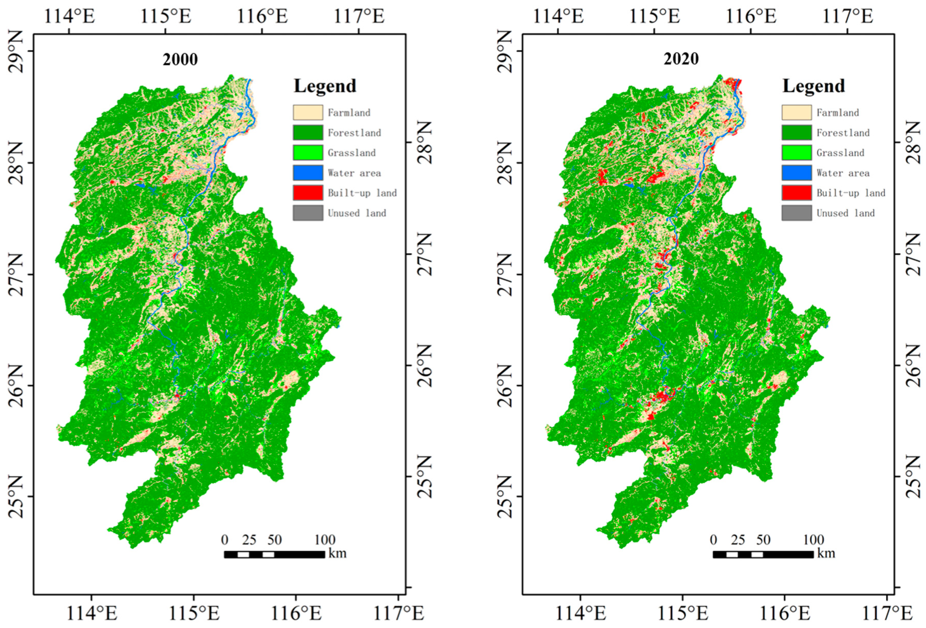
3.1. Land Use Change from 2000 to 2020

Forestland and farmland collectively occupied about 90% of the basin (Figure 2 and

Table 3. Land use composition in 2000 and 2020.

Year	2000		2020
Land Use	Area (ha)	Percent (%)	Area (ha)	Percent (%)
Farmland	2,035,057	25.10	1,988,279	24.52
Forestland	5,360,421	66.11	5,287,054	65.21
Grassland	430,096	5.30	443,763	5.47
Water area	148,182	1.83	150,005	1.85
Built-up land	133,076	1.64	237,801	2.93
Unused land	1059	0.01	989	0.01

). During the past 20 years, built-up land expanded by 78.7% (104,725 ha), while forestland and farmland decreased by 73,367 ha and 46,778 ha, respectively. Grassland and water areas experienced an increasing trend, while unused land decreased slightly. From 2000 to 2020, new built-up land mainly occupied farmland (67,659 ha) and forestland (41,734 ha) (

Table 4. Land use transition from 2000 to 2020.

Area(ha)		2020
		Farmland	Forestland	Grassland	Water Area	Built-Up Land	Unused Land
2000	Farmland	1,860,119	90,436	9052	7761	67659	30
	Forestland	98,865	5,166,929	48,013	4844	41,734	35
	Grassland	12,664	24,096	385,762	1267	6301	7
	Water area	6879	3791	653	135,726	1134	0
	Built-up land	9713	1776	276	405	120,903	3
	Unused land	39	26	8	2	71	914

). There were frequent conversions between farmland and forestland. During the past 20 years, 90,436 ha of farmland was converted into forestland, while 98,865 ha of forestland was converted into farmland. Meanwhile, a considerable amount of forestland (48,013 ha) was converted into grassland, which was approximately twice that was converted from grassland to forestland (24,096 ha). In addition, 9713 ha of built-up land has been returned to farmland.

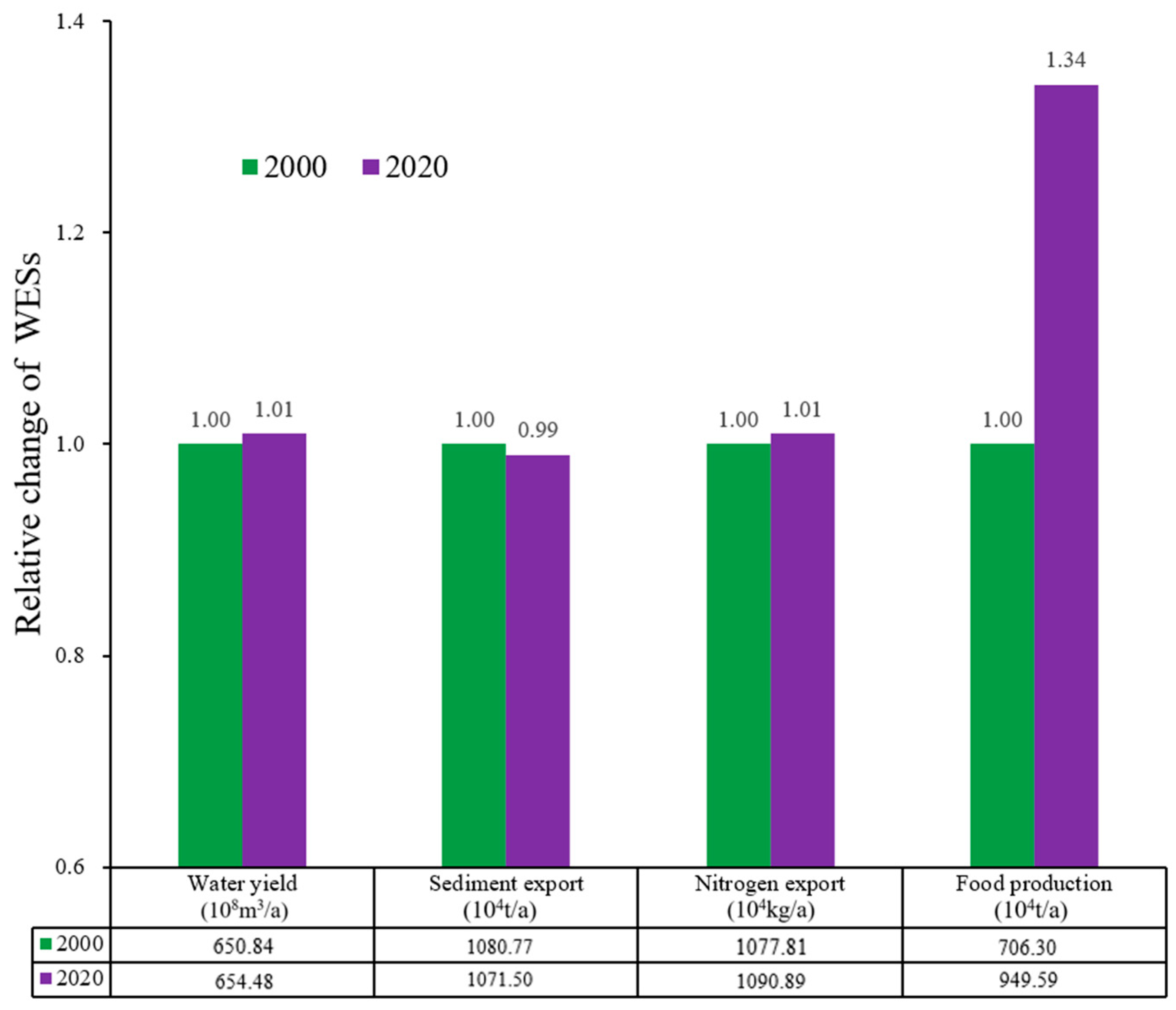
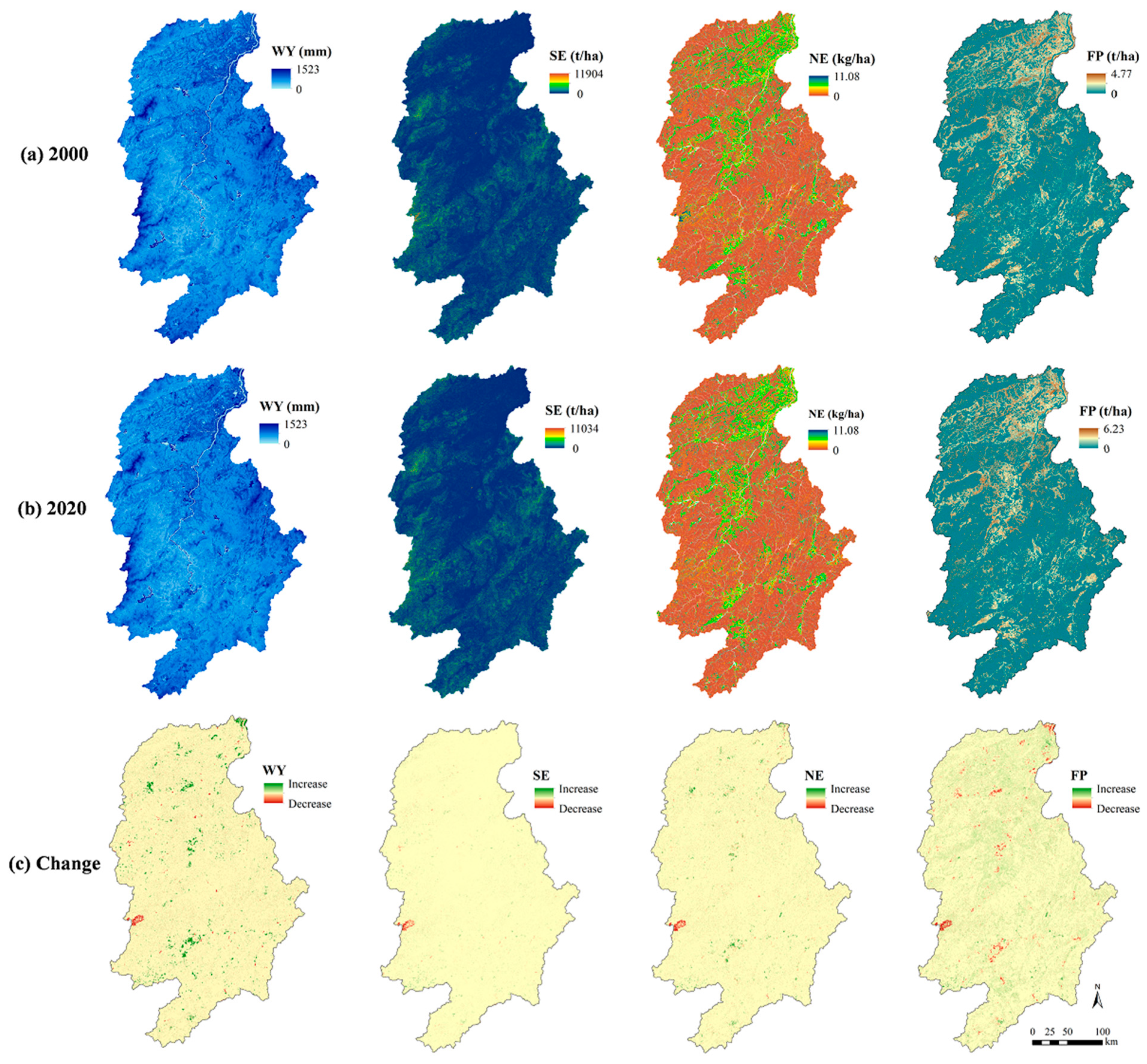
3.2. Changes in WESs from 2000 to 2020

Water yield, soil retention, and food production services were improved while the water purification service deteriorated during the past 20 years (Figure 3). Water yield increased by 0.56% from 650.84 × 10⁸ m³ in 2000 to 654.48 × 10⁸ m³ in 2020. Water yield increased mainly in the new built-up land while mainly decreasing in Guidong county of Hunan Province (Figure 4). Soil retention was improved since sediment export decreased from 1080.77 × 10⁴ t in 2000 to 1071.50 × 10⁴ t in 2020. The high value of sediment export mainly occurred in mountainous regions, while the low value mainly occurred in plain regions. The obvious reduction of sediment export occurred in Guidong county. Nitrogen export increased by 13.08 × 10⁴ kg from 2000 to 2020, indicating that water purification has improved. The high value of nitrogen export mainly occurred in farmland, while the low value mainly occurred in forestland. The obvious reduction in nitrogen export occurred in Guidong county, while the increase in nitrogen export occurred in regions where built-up land occupied forestland. Although the area of farmland decreased, food production still significantly increased by 34.45% in the GJRB during the past two decades. Although food production decreased in Guidong county and regions where built-up land occupied farmland, it significantly increased in most farmland.

3.3. Impacts of Land Use Change on WESs

The impacts of main land use conversions on WESs in the GJRB were further analyzed (

Table 5. Change in WESs induced by major land use conversions from 2000 to 2020.

Land Use Conversion	Water Yield (106 m3)	Sediment Export (104 t)	Nitrogen Export (104 kg)	Food Production (104 t)
Farmland to forestland	−197.96	−33.47	−30.03	−32.53
Forestland to farmland	217.05	20.67	29.22	49.51
Farmland to grassland	\	−0.24	−2.18	−3.00
Grassland to farmland	\	0.75	3.15	5.94
Farmland to water area	−68.46	−0.27	−2.61	−2.41
Water area to farmland	60.48	0.19	2.51	3.00
Farmland to built-up land	163.65	−2.81	−3.70	−21.72
Built-up land to farmland	−24.01	0.36	0.97	4.41
Forestland to grassland	106.09	13.77	3.53	\
Grassland to forestland	−52.71	−6.54	−1.73	\
Forestland to water area	−32.93	−0.06	−0.19	\
Water area to forestland	26.07	0.07	0.18	\
Forestland to built-up land	197.87	−0.93	9.40	\
Grassland to built-up land	15.53	−0.37	1.11	\

Note: “\” means little or no changes on WESs.

). Conversions from forestland to farmland, forestland to built-up land, farmland to built-up land, and from forestland to grassland induced an increase of 217.05 × 10⁶ m³, 197.87 × 10⁶ m³, 163.65 × 10⁶ m³, and 106.09 × 10⁶ m³ in water yield, respectively. In contrast, conversion from farmland to forestland contributed most to the decrease in water yield (−197.96 × 10⁶ m³). Afforestation significantly improved the soil retention service. Conversion from farmland and grassland to forestland induced a reduction of 33.47 × 10⁴ t and 6.54 × 10⁴ t in sediment export, respectively. Meanwhile, conversion from forestland to farmland and grassland induced an increase of 20.67 × 10⁴ t and 13.77 × 10⁴ t in sediment export, respectively. Returning farmland to forestland has induced a decline of 30.03 × 10⁴ kg in nitrogen export. However, transitions from forestland to farmland and built-up land induced a 29.22 × 10⁴ kg and 9.40 × 10⁴ kg increase in nitrogen export. Occupations of farmland by forestland and built-up land led to a reduction of 32.53 × 10⁴ t and 21.72 × 10⁴ t in food production, respectively. Meanwhile, conversion from forestland to farmland induced an increase of 49.51 × 10⁴ t in food production.

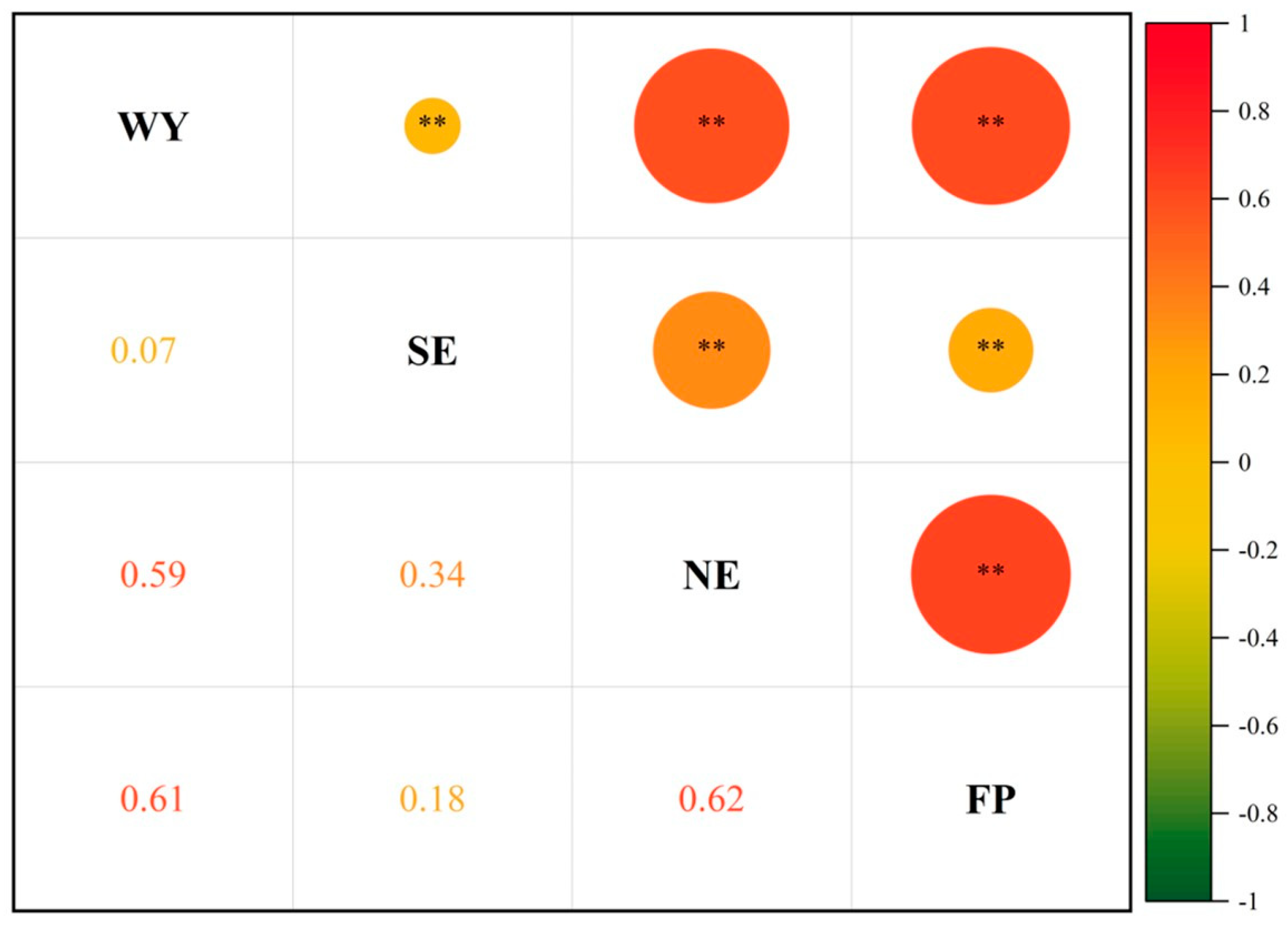
3.4. Trade-Offs and Synergies between WESs

All four selected WESs significantly correlated in 2020 (Figure 5). Food production had positive correlations with nitrogen export, and sediment export, which indicated the trade-off relationship between food production and water purification and soil retention. Food production had a synergetic relationship with water yield. Soil retention had a synergetic relationship with water purification because sediment export was positively correlated with nitrogen export. Water yield had positive correlations with sediment export and nitrogen export, which meant that water yield had a trade-off relationship with water purification and soil retention.

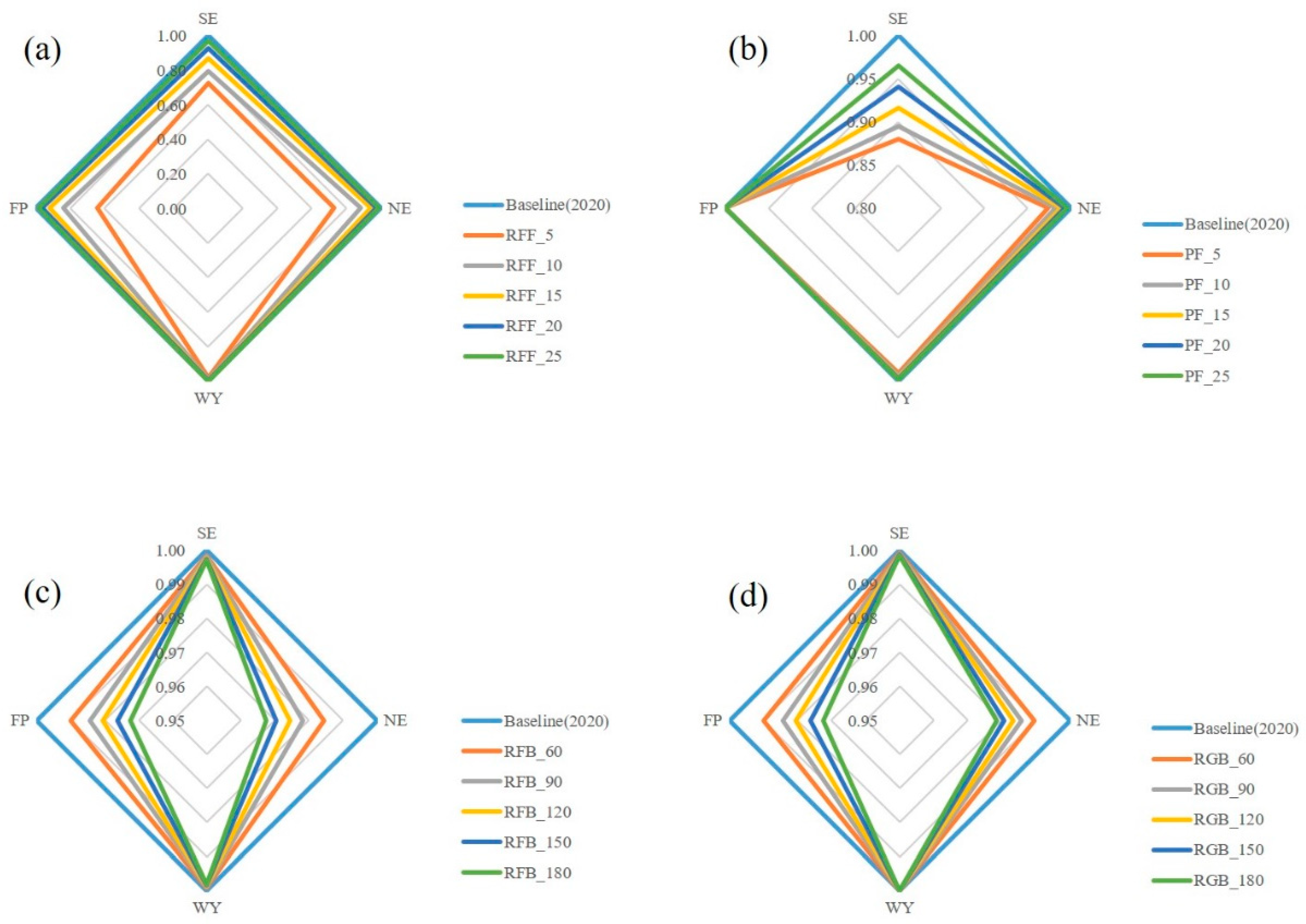
3.5. Changes in WESs under Multiple Ecological Restoration Scenarios

Water yield, sediment export, and nitrogen export decreased in all scenarios and the range of reduction increased with the increase in the intensity of ERPs (

Table 6. Change in WESs under multiple scenarios compared with 2020.

Scenario	Water Yield		Sediment Export		Nitrogen Export		Food Production
	Value (106 m3)	Percent (%)	Value (104 t)	Percent (%)	Value (104 kg)	Percent (%)	Value (104 t)	Percent (%)
RFF_5	−1347.83	−2.06	−297.00	−27.72	−295.60	−27.10	−339.25	−35.73
RFF_10	−602.41	−0.92	−219.22	−20.46	−127.32	−11.67	−155.24	−16.35
RFF_15	−299.14	−0.46	−140.85	−13.15	−63.96	−5.86	−78.31	−8.25
RFF_20	−138.08	−0.21	−76.28	−7.12	−30.39	−2.79	−36.58	−3.85
RFF_25	−54.77	−0.08	−34.08	−3.18	−12.43	−1.14	−14.66	−1.54
PF_5	−612.71	−0.94	−128.25	−11.97	−28.93	−2.65	0.00	0.00
PF_10	−419.95	−0.64	−112.62	−10.51	−19.10	−1.75	0.00	0.00
PF_15	−280.61	−0.43	−89.93	−8.39	−12.70	−1.16	0.00	0.00
PF_20	−171.64	−0.26	−63.06	−5.88	−7.80	−0.72	0.00	0.00
PF_25	−91.89	−0.14	−37.44	−3.49	−4.18	−0.38	0.00	0.00
RFB_60	−49.09	−0.07	−1.58	−0.15	−17.11	−1.57	−9.51	−1.00
RFB_90	−74.00	−0.11	−2.13	−0.20	−23.85	−2.19	−14.83	−1.56
RFB_120	−91.16	−0.14	−2.52	−0.23	−27.99	−2.57	−18.51	−1.95
RFB_150	−110.33	−0.17	−2.92	−0.27	−32.27	−2.96	−22.64	−2.38
RFB_180	−126.43	−0.19	−3.28	−0.31	−35.55	−3.26	−26.12	−2.75
RGB_60	−4.12	−0.01	−0.94	−0.09	−11.44	−1.05	−9.51	−1.00
RGB_90	−4.07	−0.01	−1.15	−0.11	−15.60	−1.43	−14.83	−1.56
RGB_120	−4.02	−0.01	−1.30	−0.12	−18.23	−1.67	−18.51	−1.95
RGB_150	−3.96	−0.01	−1.44	−0.13	−21.07	−1.93	−22.64	−2.38
RGB_180	−3.91	−0.01	−1.58	−0.15	−23.33	−2.14	−26.12	−2.75

and Figure 6). Food production decreased in all scenarios except for PF scenarios. The impact of ecological restoration on water yield was small since water yield only decreased by 0.01% to 2.06% under different scenarios compared with the baseline. Under RFF scenarios, both sediment export and nitrogen export decreased significantly while food production decreased. Under the RFF_5 scenario, sediment export and nitrogen export decreased by 27.72% (297 × 10⁴ t) and 27.10% (295.60 × 10⁴ kg), respectively. Under PF scenarios, the reduction in nitrogen export was much lower than that of sediment export. This indicated that afforestation can effectively improve soil retention, but has relatively little effect on water purification. Under the PF_5 scenario, sediment export and nitrogen export decreased by 11.97% (128.25 × 10⁴ t) and 2.65% (28.93 × 10⁴ kg), respectively. Under RFB scenarios and RGB scenarios, the reduction of nitrogen export was much higher than that of sediment export. This indicated that river vegetation buffers can effectively improve water purification, but have little effect on soil conservation. Moreover, the decrease in nitrogen export and sediment export under RFB scenarios was larger than that under RGB scenarios at the same intensity. Under the RFB_180 scenario, sediment export and nitrogen export decreased by 0.31% (3.28 × 10⁴ t) and 3.26% (35.55 × 10⁴ kg), respectively. In comparison, the RGB_180 scenario sediment export and nitrogen export only decreased by 0.15% (1.58 × 10⁴ t) and 2.14% (23.33 × 10⁴ kg), respectively.

4. Discussion

4.1. Changes in Land Use Change and WESs

The GJRB is a typical subtropical mountainous region with serious soil erosion. To control soil erosion, many ERPs have been launched in this basin, which promoted forestland expansion [45,46]. In GJRB, 90,436 ha of farmland and 24,096 ha of grassland have been converted into forestland from 2000 to 2020. With rapid urbanization, built-up land expanded by 78.7%, which was mainly converted from farmland (67,659 ha) and forestland (41,734 ha). Meanwhile, considerable forestland, grassland, and water areas have been transferred into farmland. This should be mainly attributed to the ‘requisition-compensation balance of farmland’ (RCBF) policy [47]. Although this policy can contribute to food security, it also facilitates the occupation of ecological land by farmland, which undoubtedly will pose a negative impact on the ESs [48,49].

Land use change significantly affected WESs in the GJRB. Water yield, soil retention, and food production improved while water purification deteriorated from 2000 to 2020. Forestland expansion significantly improved soil retention. Conversion from farmland to forestland led to a reduction of 33.47 × 10⁴ t in sediment export. On the one hand, forest canopy and litter can intercept precipitation and reduce rainfall erosivity [50]. On the other hand, the complex root system of forests can stabilize soil to improve soil stability and reduce soil erodibility [3]. In addition, grassland afforestation has also effectively reduced sediment export. These results indicated that ERPs have achieved good benefits in controlling soil erosion in the GJRB, which was in accordance with previous studies [42,51]. However, deforestation resulted in an increment in sediment export, which has almost offset the positive effect of ERPs. In this study, conversions from forestland to farmland and grassland induced an increment in sediment export by 20.67 × 10⁴ t and 13.77 × 10⁴ t, respectively. Because of the RCBF policy, the occupied farmland must be compensated to keep the farmland area from decreasing. However, due to economic development considerations, the land on the plain tends to transfer into built-up land rather than farmland. As a result, considerable ecological land in mountainous areas has been transformed into farmland. It is noteworthy that more than half of the new farmland had a slope greater than 5 degrees in the basin from 2000 to 2020 (Figure 7), which resulted in serious soil erosion. Chen, et al. [52] indicated that the mean elevation of farmland in China has increased by 17.38 m during the past four decades. Kong, et al. [49] indicated that farmland reclamation has undermined gains in various ESs in China from 2000 to 2015. The ERPs have improved water quality. In this study, the conversion from farmland to forestland induced a reduction of 30.03 × 10⁴ kg in nitrogen export. Farmland has been considered the main source of nutrient pollution in China [7,31,53]. Forestland can reduce runoff and soil erosion, thereby reducing nutrient output. Moreover, the nutrient absorption capacity of forestland is much higher than that of other land use types. In GJRB, conversion from farmland to built-up land improved water quality, while conversion from forestland to built-up land induced water quality deterioration. This was consistent with previous studies [35,54]. From 2000 to 2020, water yield increased by 0.56% in GJRB. Returning farmland to forestland contributed most to the decrease in water yield, while water yield increased mainly because of deforestation and built-up land expansion. The GJRB is a subtropical mountainous basin with sufficient precipitation. Increase in water yield may aggravate the regional flood risk. Although the area of farmland decreased, the food production significantly increased by 34.45% from 2000 to 2020. This should be attributed to the development of modern agriculture technology and the application of fertilization. This indicated that the change in farmland area is not the main factor affecting food production. Some previous studies also support this conclusion [18,55].

4.2. Impact of Ecological Restoration on WESs

Previous studies indicated that ERPs can increase evapotranspiration, thereby decreasing water yield [23]. In this study, water yield decreased slightly under all scenarios, with a range from 0.01% to 2.06%. In arid regions, the decrease in water yield may threaten water security and induce ecosystem degradation [31]. In contrast, it may reduce the flood risk in humid regions like the GJRB. Many studies indicated that the restoration of riparian vegetation could effectively improve soil retention and water purification [7,56]. However, we found that the improvement in soil retention was relatively much smaller than that of water purification in the RFB and RGB scenarios. The reason was that, on the one hand, the GJRB is a large basin with an area of more than 80,000 km², and the riparian buffer zone accounts for a small proportion of the area. On the other hand, soil erosion is serious in the GJRB, but the proportion of soil erosion occurring in the riparian buffer zone mainly located in plain areas is also very small. This indicated that an ERP suitable for one region may not be suitable for another region. The optimal type of ERPs must be determined according to local environmental conditions. At the same intensity, RFB scenarios have a better effect on improving water purification service than RGB scenarios. This is because forestland has better nitrogen absorption and retention capacity than grassland [31]. The PF scenarios can effectively improve soil retention but have little effect on water purification. The reason was that grassland is not the main source of nutrient pollution, which has low nitrogen input and high nitrogen retention [32]. Under RFF scenarios, soil retention and water purification can be simultaneously improved. This indicated that RFF is the optimal ecological restoration type in the GJRB. Qi, et al. [6] reported that returning farmland with a slope greater than 25° to forestland can reduce sediment export by 27.07% in the Hanjiang River basin. However, we found that sediment export can only be reduced by 3.18% under the same scenario (RFF_25 scenario) in the GJRB. This indicated that the intensity of ERPs must be determined based on local characteristics. In addition, returning farmland to forestland results in a decline in the area of farmland, which undoubtedly affects food production [24,31]. Policymakers need to select suitable ERPs to achieve a balance between ecological conservation and food security. Under the RFF_5 scenario, although sediment export and nitrogen export improved significantly, the food production decreased by as much as 35.73%, which will threaten local food security. Comprehensively considering ecological security and food security, the RFF_10 should be the optimal scenario in the study area.

4.3. Implications

Previous studies indicated that unsuitable ERPs may lead to ecosystem degradation [20,21]. Determining suitable ERPs is the key to ecological restoration and sustainable development, especially in ecologically fragile regions. Previous studies mainly focus on the impacts of either type [7,18] or intensity [20,36] of ERPs on ESs. In this study, we comprehensively considered the type and intensity of ERPs and determined the optimal ecological restoration scenario in the GJRB, which can provide useful information for local ecosystem management. This study highlights that both the type and intensity of ERPs should be taken into consideration in ecological restoration. In general, farmland with a slope greater than 25° was converted to forestland to control soil erosion in China. However, our results indicated that this intensity is not enough to effectively reduce sediment export in subtropical mountainous regions. The intensity of ERPs must be determined according to local ecological characteristics. The GJRB is an ecologically fragile region, and the trade-off between food production and regulation services (i.e., soil retention and water purification) should be the primary concern of policymakers. This study indicated that change in the area of farmland was not the dominant factor affecting food production in the GJRB. It is not wise to increase food production through farmland expansion because it will result in degradation in soil retention and water purification. In this study, farmland expansion induced by the RCBF policy has almost offset the benefits of ERPs during the past 20 years. Therefore, the RCBF policy should be reconsidered, especially in mountainous regions. Local policymakers should achieve a balance between food production and ecological protection. The RFF should be used as the primary ecological restoration measure for the entire basin. In plain areas, RFB should be used as a complementary measure to reduce water pollution. In contrast, in mountainous areas, PF should be used as a complementary measure to reduce soil erosion. In addition, building terraces on steep slopes can also effectively reduce soil erosion [51]. Establishing farmland shelterbelts can also effectively improve WESs. Previous studies indicated that farmland shelterbelts can not only improve fertilizer use efficiency to reduce water pollution but also significantly increase crop yield [55].

4.4. Limitations

There remain some limitations in this study. Firstly, the InVEST model simplified hydrological processes, which may result in uncertainties in ES evaluation [41]. Specifically, the AWY module calculates water yield by using annual average climate data, which ignores the temporal dimensions of water provision. The SDR module only considers rill/inter-rill erosion processes while ignoring gully erosion, stream bank erosion, and mass erosion. The NDR module only considers filtration by vegetation while ignoring the biochemical processes of nutrients in streams, which would lead to an underestimation of nutrient retention in the delivery process. Therefore, we used observed data from the hydrological station to validate the AWY module and SDR module to reduce uncertainties. For the NDR module, due to a lack of observed data, we derived parameters from previous research conducted in regions adjacent to GJRB [18]. Secondly, the data sources of this study are diverse. For example, NDVI comes from MODIS data with a spatial resolution of 250 m, and the spatial resolution of climate data and soil data was 1 km. Although all data were resampled at the same resolution, it may bring some uncertainties. Thirdly, this study only evaluated four WESs, while flood regulation was not considered due to a lack of available data and model. Floods occurred frequently and induced considerable economic loss in the GJRB [39]. Therefore, flood regulation should be considered in the future to better support ecosystem management and sustainable development.

5. Conclusions

In this study, we analyzed the impact of land use change on four WESs in GJRB from 2000 to 2020. Furthermore, comprehensively considering the type and intensity of ERPs, we designed multiple scenarios to explore the impact of ecological restoration on WESs. The results revealed that water yield, soil retention, and food production increased while water purification decreased due to land use change from 2000 to 2020. Conversions from forestland to farmland and built-up land were two main contributors to water quality deterioration. Trade-offs only occurred between regulating services and provisioning services. Among ecological restoration scenarios, the RFF scenarios were optimal because they can simultaneously significantly improve soil retention and water purification, although they will result in a reduction in food production. Considering food security, the RFF_10 scenario was the best in this study. Both the type and intensity of ERPs should be considered in ecological restoration. In addition, we recommend that the RCBF policy should be limited, especially in mountainous regions like GJRB.

References

1. Costanza, R.; d’Arge, R.; de Groot, R.; Farber, S.; Grasso, M.; Hannon, B.; Limburg, K.; Naeem, S.; O’Neill, R.V.; Paruelo, J.; et al. The value of the world’s ecosystem services and natural capital. Nature 1997, 387, 253–260. [Google Scholar] [CrossRef]
2. Maestre, F.T.; Le Bagousse-Pinguet, Y.; Delgado-Baquerizo, M.; Eldridge, D.J.; Saiz, H.; Berdugo, M.; Gozalo, B.; Ochoa, V.; Guirado, E.; Garcia-Gomez, M.; et al. Grazing and ecosystem service delivery in global drylands. Science 2022, 378, 915–920. [Google Scholar] [CrossRef] [PubMed]
3. Felipe-Lucia, M.R.; Soliveres, S.; Penone, C.; Fischer, M.; Ammer, C.; Boch, S.; Boeddinghaus, R.S.; Bonkowski, M.; Buscot, F.; Fiore-Donno, A.M.; et al. Land-use intensity alters networks between biodiversity, ecosystem functions, and services. Proc. Natl. Acad. Sci. USA 2020, 117, 28140–28149. [Google Scholar] [CrossRef]
4. van Vliet, J. Direct and indirect loss of natural area from urban expansion. Nat. Sustain. 2019, 2, 755–763. [Google Scholar] [CrossRef]
5. Reid, W.V.; Mooney, H.A.; Cropper, A.; Capistrano, D.; Carpenter, S.R.; Chopra, K.; Dasgupta, P.; Dietz, T.; Duraiappah, A.K.; Hassan, R.; et al. Ecosystems and Human Well-being: Synthesis; Island Press: Washington, DC, USA, 2005. [Google Scholar]
6. Qi, W.; Li, H.; Zhang, Q.; Zhang, K. Forest restoration efforts drive changes in land-use/land-cover and water-related ecosystem services in China’s Han River basin. Ecol. Eng. 2019, 126, 64–73. [Google Scholar] [CrossRef]
7. Gao, J.; Li, F.; Gao, H.; Zhou, C.; Zhang, X. The impact of land-use change on water-related ecosystem services: A study of the Guishui River Basin, Beijing, China. J. Clean. Prod. 2017, 163, S148–S155. [Google Scholar] [CrossRef]
8. Ouyang, Z.; Zheng, H.; Xiao, Y.; Polasky, S.; Liu, J.; Xu, W.; Wang, Q.; Zhang, L.; Xiao, Y.; Rao, E.; et al. Improvements in ecosystem services from investments in natural capital. Science 2016, 352, 1455–1459. [Google Scholar] [CrossRef] [PubMed]
9. Rey Benayas, J.M.; Newton, A.C.; Diaz, A.; Bullock, J.M. Enhancement of Biodiversity and Ecosystem Services by Ecological Restoration: A Meta-Analysis. Science 2009, 325, 1121–1124. [Google Scholar] [CrossRef]
10. Lei, J.-C.; Wang, S.; Wu, J.; Wang, J.-W.; Xiong, X. Land-use configuration has significant impacts on water-related ecosystem services. Ecol. Eng. 2021, 160, 106133. [Google Scholar] [CrossRef]
11. Zhou, M.; Deng, J.; Lin, Y.; Zhang, L.; He, S.; Yang, W. Evaluating combined effects of socio-economic development and ecological conservation policies on sediment retention service in the Qiantang River Basin, China. J. Clean. Prod. 2021, 286, 124961. [Google Scholar] [CrossRef]
12. Gou, M.; Li, L.; Ouyang, S.; Wang, N.; La, L.; Liu, C.; Xiao, W. Identifying and analyzing ecosystem service bundles and their socioecological drivers in the Three Gorges Reservoir Area. J. Clean. Prod. 2021, 307, 127208. [Google Scholar] [CrossRef]
13. Wang, Y.; Zhang, Z.; Chen, X. Land Use Transitions and the Associated Impacts on Carbon Storage in the Poyang Lake Basin, China. Remote Sens. 2023, 15, 2703. [Google Scholar] [CrossRef]
14. Yang, Y. Evolution of habitat quality and association with land-use changes in mountainous areas: A case study of the Taihang Mountains in Hebei Province, China. Ecol. Indic. 2021, 129, 107967. [Google Scholar] [CrossRef]
15. Ma, S.; Wang, L.-J.; Jiang, J.; Zhao, Y.-G. Land use/land cover change and soil property variation increased flood risk in the black soil region, China, in the last 40 years. Environ. Impact Assess. Rev. 2024, 104, 107314. [Google Scholar] [CrossRef]
16. Lu, F.; Hu, H.; Sun, W.; Zhu, J.; Liu, G.; Zhou, W.; Zhang, Q.; Shi, P.; Liu, X.; Wu, X.; et al. Effects of national ecological restoration projects on carbon sequestration in China from 2001 to 2010. Proc. Natl. Acad. Sci. USA 2018, 115, 4039–4044. [Google Scholar] [CrossRef] [PubMed]
17. Bennett, E.M.; Peterson, G.D.; Gordon, L.J. Understanding relationships among multiple ecosystem services. Ecol. Lett. 2009, 12, 1394–1404. [Google Scholar] [CrossRef] [PubMed]
18. Liang, J.; Li, S.; Li, X.; Li, X.; Liu, Q.; Meng, Q.; Lin, A.; Li, J. Trade-off analyses and optimization of water-related ecosystem services (WRESs) based on land use change in a typical agricultural watershed, southern China. J. Clean. Prod. 2021, 279, 123851. [Google Scholar] [CrossRef]
19. Yang, S.Q.; Zhao, W.W.; Liu, Y.X.; Wang, S.; Wang, J.; Zhai, R.J. Influence of land use change on the ecosystem service trade-offs in the ecological restoration area: Dynamics and scenarios in the Yanhe watershed, China. Sci. Total Environ. 2018, 644, 556–566. [Google Scholar] [CrossRef]
20. Peng, J.; Hu, X.; Wang, X.; Meersmans, J.; Liu, Y.; Qiu, S. Simulating the impact of Grain-for-Green Programme on ecosystem services trade-offs in Northwestern Yunnan, China. Ecosyst. Serv. 2019, 39, 100998. [Google Scholar] [CrossRef]
21. Divinsky, I.; Becker, N.; Bar, P. Ecosystem service tradeoff between grazing intensity and other services—A case study in Karei-Deshe experimental cattle range in northern Israel. Ecosyst. Serv. 2017, 24, 16–27. [Google Scholar] [CrossRef]
22. Raudsepp-Hearne, C.; Peterson, G.D.; Bennett, E.M. Ecosystem service bundles for analyzing tradeoffs in diverse landscapes. Proc. Natl. Acad. Sci. USA 2010, 107, 5242–5247. [Google Scholar] [CrossRef] [PubMed]
23. Feng, X.; Fu, B.; Piao, S.; Wang, S.; Ciais, P.; Zeng, Z.; Lü, Y.; Zeng, Y.; Li, Y.; Jiang, X.; et al. Revegetation in China’s Loess Plateau is approaching sustainable water resource limits. Nat. Clim. Chang. 2016, 6, 1019–1022. [Google Scholar] [CrossRef]
24. Chen, Y.; Wang, K.; Lin, Y.; Shi, W.; Song, Y.; He, X. Balancing green and grain trade. Nat. Geosci. 2015, 8, 739–741. [Google Scholar] [CrossRef]
25. Villa, F.; Bagstad, K.J.; Voigt, B.; Johnson, G.W.; Portela, R.; Honzák, M.; Batker, D. A Methodology for Adaptable and Robust Ecosystem Services Assessment. PLoS ONE 2014, 9, e91001. [Google Scholar] [CrossRef] [PubMed]
26. Jiang, Y.; Gao, J.; Wu, S.; Jiao, K. Mediation effect as the component to ecosystem? Establishing the chain effect framework of ecosystem services across typical karst basin in China. Catena 2023, 221, 106761. [Google Scholar] [CrossRef]
27. Verma, S.; Verma, M.K.; Prasad, A.D.; Mehta, D.J.; Islam, M.N. Modeling of uncertainty in the estimation of hydrograph components in conjunction with the SUFI-2 optimization algorithm by using multiple objective functions. Model. Earth Syst. Environ. 2024, 10, 61–79. [Google Scholar] [CrossRef]
28. Hamel, P.; Chaplin-Kramer, R.; Sim, S.; Mueller, C. A new approach to modeling the sediment retention service (InVEST 3.0): Case study of the Cape Fear catchment, North Carolina, USA. Sci. Total Environ. 2015, 524–525, 166–177. [Google Scholar] [CrossRef] [PubMed]
29. Chen, D.; Jiang, P.; Li, M. Assessing potential ecosystem service dynamics driven by urbanization in the Yangtze River Economic Belt, China. J Env. Manag. 2021, 292, 112734. [Google Scholar] [CrossRef]
30. Bai, Y.; Ochuodho, T.O.; Yang, J. Impact of land use and climate change on water-related ecosystem services in Kentucky, USA. Ecol. Indic. 2019, 102, 51–64. [Google Scholar] [CrossRef]
31. Ma, S.; Wang, L.-J.; Chu, L.; Jiang, J. Determination of ecological restoration patterns based on water security and food security in arid regions. Agric. Water Manag. 2023, 278, 108171. [Google Scholar] [CrossRef]
32. Zheng, H.; Wang, L.; Peng, W.; Zhang, C.; Li, C.; Robinson, B.E.; Wu, X.; Kong, L.; Li, R.; Xiao, Y.; et al. Realizing the values of natural capital for inclusive, sustainable development: Informing China’s new ecological development strategy. Proc. Natl. Acad. Sci. USA 2019, 116, 8623–8628. [Google Scholar] [CrossRef] [PubMed]
33. Wang, Y.; Zhang, Z.; Chen, X. Spatiotemporal change in ecosystem service value in response to land use change in Guizhou Province, southwest China. Ecol. Indic. 2022, 144, 109514. [Google Scholar] [CrossRef]
34. Verma, S.; Verma, M.K.; Prasad, A.D.; Mehta, D.; Azamathulla, H.M.; Muttil, N.; Rathnayake, U. Simulating the Hydrological Processes under Multiple Land Use/Land Cover and Climate Change Scenarios in the Mahanadi Reservoir Complex, Chhattisgarh, India. Water 2023, 15, 3068. [Google Scholar] [CrossRef]
35. Sun, X.; Crittenden, J.C.; Li, F.; Lu, Z.M.; Dou, X.L. Urban expansion simulation and the spatio-temporal changes of ecosystem services, a case study in Atlanta Metropolitan area, USA. Sci. Total Environ. 2018, 622, 974–987. [Google Scholar] [CrossRef]
36. Ma, S.; Qiao, Y.-P.; Jiang, J.; Wang, L.-J.; Zhang, J.-C. Incorporating the implementation intensity of returning farmland to lakes into policymaking and ecosystem management: A case study of the Jianghuai Ecological Economic Zone, China. J. Clean. Prod. 2021, 306, 127284. [Google Scholar] [CrossRef]
37. Wen, T.; Xiong, L.; Jiang, C.; Hu, J.; Liu, Z. Effects of Climate Variability and Human Activities on Suspended Sediment Load in the Ganjiang River Basin, China. J. Hydrol. Eng. 2019, 24, 05019029. [Google Scholar] [CrossRef]
38. He, X.; Miao, Z.; Wang, Y.; Yang, L.; Zhang, Z. Response of soil erosion to climate change and vegetation restoration in the Ganjiang River Basin, China. Ecol. Indic. 2024, 158, 111429. [Google Scholar] [CrossRef]
39. Liu, X.; Zhang, L.; She, D.; Chen, J.; Xia, J.; Chen, X.; Zhao, T. Postprocessing of hydrometeorological ensemble forecasts based on multisource precipitation in Ganjiang River basin, China. J. Hydrol. 2022, 605, 127323. [Google Scholar] [CrossRef]
40. Hu, H.; Jin, D.; Yang, Y.; Zhang, J.; Ma, C.; Qiu, Z. Distinct profile of bacterial community and antibiotic resistance genes on microplastics in Ganjiang River at the watershed level. Environ. Res. 2021, 200, 111363. [Google Scholar] [CrossRef]
41. NCP. InVEST 3.13.0 User’s Guide; Stanford University, University of Minnesota, Chinese Academy of Sciences, The Nature Conservancy, World Wildlife Fund, and Stockholm Resilience Centre: Stanford, CA, USA, 2022. [Google Scholar]
42. Li, J.; Xie, B.; Gao, C.; Zhou, K.; Liu, C.; Zhao, W.; Xiao, J.; Xie, J. Impacts of natural and human factors on water-related ecosystem services in the Dongting Lake Basin. J. Clean. Prod. 2022, 370, 133400. [Google Scholar] [CrossRef]
43. Wang, Y.; Wang, H.; Zhang, J.; Liu, G.; Fang, Z.; Wang, D. Exploring interactions in water-related ecosystem services nexus in Loess Plateau. J. Environ. Manag. 2023, 336, 117550. [Google Scholar] [CrossRef]
44. Xia, H.; Yuan, S.; Prishchepov, A.V. Spatial-temporal heterogeneity of ecosystem service interactions and their social-ecological drivers: Implications for spatial planning and management. Resour. Conserv. Recycl. 2023, 189, 106767. [Google Scholar] [CrossRef]
45. Wang, Y.; Zhang, Z.; Chen, X. Quantifying Influences of Natural and Anthropogenic Factors on Vegetation Changes Based on Geodetector: A Case Study in the Poyang Lake Basin, China. Remote Sens. 2021, 13, 5081. [Google Scholar] [CrossRef]
46. Ning, K.; Chen, J.; Li, Z.; Liu, C.; Nie, X.; Liu, Y.; Wang, L.; Hu, X. Land use change induced by the implementation of ecological restoration Programs increases future terrestrial ecosystem carbon sequestration in red soil hilly region of China. Ecol. Indic. 2021, 133, 108409. [Google Scholar] [CrossRef]
47. Shen, X.; Wang, L.; Wu, C.; Lv, T.; Lu, Z.; Luo, W.; Li, G. Local interests or centralized targets? How China’s local government implements the farmland policy of Requisition–Compensation Balance. Land Use Policy 2017, 67, 716–724. [Google Scholar] [CrossRef]
48. Chen, W.; Ye, X.; Li, J.; Fan, X.; Liu, Q.; Dong, W. Analyzing requisition–compensation balance of farmland policy in China through telecoupling: A case study in the middle reaches of Yangtze River Urban Agglomerations. Land Use Policy 2019, 83, 134–146. [Google Scholar] [CrossRef]
49. Kong, L.; Wu, T.; Xiao, Y.; Xu, W.; Zhang, X.; Daily, G.C.; Ouyang, Z. Natural capital investments in China undermined by reclamation for cropland. Nat. Ecol. Evol. 2023, 7, 1771–1777. [Google Scholar] [CrossRef] [PubMed]
50. Chen, H.; Zhang, X.; Abla, M.; Lu, D.; Yan, R.; Ren, Q.; Ren, Z.; Yang, Y.; Zhao, W.; Lin, P.; et al. Effects of vegetation and rainfall types on surface runoff and soil erosion on steep slopes on the Loess Plateau, China. Catena 2018, 170, 141–149. [Google Scholar] [CrossRef]
51. Huang, C.; Zhao, D.; Liao, Q.; Xiao, M. Linking landscape dynamics to the relationship between water purification and soil retention. Ecosyst. Serv. 2023, 59, 101498. [Google Scholar] [CrossRef]
52. Chen, W.; Yang, L.; Zeng, J.; Yuan, J.; Gu, T.; Liu, Z. Untangling the increasing elevation of cropland in China from 1980 to 2020. Geogr. Sustain. 2023, 4, 281–293. [Google Scholar] [CrossRef]
53. Guo, M.; Ma, S.; Wang, L.-J.; Lin, C. Impacts of future climate change and different management scenarios on water-related ecosystem services: A case study in the Jianghuai ecological economic Zone, China. Ecol. Indic. 2021, 127, 107732. [Google Scholar] [CrossRef]
54. Sun, X.; Lu, Z.; Li, F.; Crittenden, J.C. Analyzing spatio-temporal changes and trade-offs to support the supply of multiple ecosystem services in Beijing, China. Ecol. Indic. 2018, 94, 117–129. [Google Scholar] [CrossRef]
55. Yang, S.; Bai, Y.; Alatalo, J.M.; Wang, H.; Jiang, B.; Liu, G.; Chen, J. Spatio-temporal changes in water-related ecosystem services provision and trade-offs with food production. J. Clean. Prod. 2021, 286, 125316. [Google Scholar] [CrossRef]
56. Zheng, H.; Li, Y.F.; Robinson, B.E.; Liu, G.; Ma, D.C.; Wang, F.C.; Lu, F.; Ouyang, Z.Y.; Daily, G.C. Using ecosystem service trade-offs to inform water conservation policies and management practices. Front. Ecol. Environ. 2016, 14, 527–532. [Google Scholar] [CrossRef]
Figure 1. Location (a) and elevation (b) of the GJRB.
Forests 15 01225 g001
Figure 2. Land use patterns in 2000 and 2020.
Forests 15 01225 g002
Figure 3. Values and relative changes of WESs from 2000 to 2020.
Forests 15 01225 g003
Figure 4. Spatial patterns and changes of WESs from 2000 to 2020. (a) WESs in 2000; (b) WESs in 2020; and (c) change in WESs from 2000 to 2020. (WY: water yield; SE: sediment export; NE: nitrogen export; and FP: food production).
Forests 15 01225 g004
Figure 5. Spearman’s correlations between pairs of WESs in 2020 (** p < 0.01). (WY: water yield; SE: sediment export; NE: nitrogen export; and FP: food production).
Forests 15 01225 g005
Figure 6. Trade-offs among WESs under multiple scenarios. (a) RFF scenarios; (b) PF scenarios; (c) RFB scenarios; and (d) RGB scenarios. (WY: water yield; SE: sediment export; NE: nitrogen export; and FP: food production).
Forests 15 01225 g006
Figure 7. Slope of the newly added farmland from 2000 to 2020.
Forests 15 01225 g007