Article

Sensitivity of Fire Indicators on Forest Inventory Plots Is Affected by Fire Severity and Time since Burning

Northern Research Station, USDA Forest Service, 271 Mast Road, Durham, NH 09824, USA
*
Author to whom correspondence should be addressed.
Forests 2024, 15(7), 1264; https://doi.org/10.3390/f15071264 (registering DOI)
Submission received: 11 June 2024 / Revised: 5 July 2024 / Accepted: 17 July 2024 / Published: 20 July 2024
(This article belongs to the Section Natural Hazards and Risk Management)

Abstract

:
Forest inventory data are useful for determining forest stand structure, growth, and change. Among the information collected on forest inventory plots by the USDA Forest Service Forest Inventory and Analysis Program, attributes characterizing various types of disturbance provide researchers a means of selecting plots specifically affected by disturbances, such as fire. We determine the performance of three of these attributes as indicators of recent fires on forest inventory plots of the United States by comparing them to independent records of wildland fire occurrence. The indicators are plot-level observations of fire effects on (1) general site appearance, (2) tree mortality, and (3) damage to live trees. Independent spatial layers of wildland fire perimeters provide an approach to test indicator performance and identify characteristics of fires that may affect detection. The sensitivities of indicators are generally higher in the West relative to the East. Detection rates exceed 90 percent for the Pacific Coast forests but seldom reach 80 percent in the East. Among the individual indicators, site appearance has higher identification rates than tree indicators for fires in the Pacific Coast, Great Plains, North, and South regions. Tree mortality is the most important single indicator for identifying Rocky Mountain fires. Tree damage is more important than tree mortality in the South; otherwise, the tree damage indicator is of relatively lower importance, particularly where high-severity fires are common, and tree survival is low. The rate of detection by the indicators is affected by the severity of the fire or the recency of the fire. The joint effect of severity and recency influence all three indicators for the Pacific Coast and Rocky Mountain fires, as well as the site appearance indicator in the South. Only a small proportion of fires are clearly missed by all three of the indicators.

1. Introduction

Forests experience a variety of disturbances, including insects and disease, drought, fire, and management. Fire is becoming an increasingly important disturbance because of increases in the length of the fire season and the frequency of wildfires [1,2,3,4]. Climate change is likely to increase the role of fire as an agent of forest disturbance [5,6,7]. Fire can have a variety of effects on forest ecosystems, depending on the type and severity of the fire; for example, a ground fire may have beneficial effects, such as maintaining stand density at a level appropriate for the forest type, promoting regeneration, or reducing competing vegetation. A high-severity crown fire can be a stand-replacing event, and wildfires may have negative impacts on water resources [8,9], soil health [10], and forest regeneration [11], potentially resulting in a transition to a different vegetation type [12]. Wildfire also affects stand characteristics, growth, and species composition in a variety of ways and can affect the ability of the forest to provide ecosystem services such as carbon storage, timber production, wildlife habitat, recreation opportunities, and clean air and water [13,14].
Because of the many possible effects of fire on forest resources and the increasing frequency and extent of wildfires, an easily implemented approach using existing data is needed to identify fire-affected forests and characterize the effects of fire. Spatial datasets delineating fire occurrence, extent, and severity are developed from remote sensing products. A widely used data source is the Monitoring Trends in Burn Severity data (MTBS), which uses burn indexes derived from remotely sensed reflectance data [15] to deliver wildland fire data products needed by managers. However, wildland fire layers can lack the structure or stand composition detail needed to better understand the ecological and growth impacts of wildfire on forests. Field inventory plots, such as the permanent inventory plots established and measured by the Forest Inventory and Analysis (FIA) Program of the United States Department of Agriculture Forest Service [16,17], can provide detailed information at the plot and individual tree levels. Data on key processes and features, such as growth, survival, species composition, mortality, and seedling recruitment, are collected. Observations collected on plots include information on tree damage (multiple codes are available to record disturbance and mortality agents) and various plot condition factors, including the presence of disturbance and disturbance type, as well as indicators of recent fires. FIA data have not traditionally been used to understand the effects of fire on tree, stand, and forest growth and development, but more investigators have begun exploring the use of different plot and tree variables in the FIA database (often in conjunction with remote sensing products) to examine the effects of wildfire and other disturbances on the nation’s forests [18,19,20,21,22,23].
Wildland fire perimeter records can, in some cases, be paired with the permanent forest inventory plots. We identified where these separate data sources align and described the sensitivity of plot-level fire indicators to the fire perimeter records and possible effects on sensitivity that are associated with features in either data source. While this study focused on the conterminous United States and employs FIA and MTBS data, note that this approach (with some adjustments) can be applied in any nation or region where spatial data on fire extent and forest inventory data that includes information on disturbance are available. For example, Canada maintains a national forest inventory [24] where information on disturbance effects at the plot level, including fire, is collected and also maintains the Canadian Wildfire Information System.
Our goal was to assess the performance of three different indicators of recent fires to identify FIA plots where recent fires have occurred: site condition, tree mortality, and tree damage. In addition, we examined the effect of time since fire and burn severity class on indicator performance. The indicators we evaluated can provide researchers with a means of selecting plots specifically affected by fire for further analysis.

2. Methods

2.1. Scope

This study focused on the site appearance, tree mortality, and tree damage indicators of recent fires, which are included with data collected by FIA field crews on forest plots in the nationwide network of permanent FIA inventory plots. For this analysis, the primary data sets were (1) forest inventory plot data from the FIA database, (2) wildland fire perimeter records, and (3) images indicating burn severity and forest cover on these burn perimeters. The regional summaries presented included only forest land of the conterminous United States (CONUS, 48 states, Figure 1). The Great Plains fires are considered western by MTBS, but their forests and fires are more characteristically eastern, so they are included in ‘East’ for any East–West summaries below.

2.2. Forest Inventory Plots

Forest inventory plots are described in the Forest Inventory and Analysis Database (FIADB, [16,17]) compiled and maintained by FIA. Plots are established, maintained, and continuously systematically sampled over all land within individual states so that a portion of the survey data is collected each year on a continuous series of cycles, with remeasurement intervals at 5, 7, or 10 years depending on the state [25] (see Figure S1 for plot layout). For plots on forest land, a large set of measurements and observations are collected to characterize the ecosystem, site, stand, and each tally tree (trees measured on plots). For example, data collected include forest type, elevation, stand size, stand age, individual tree species, and tree size. Included in these plot data are assessments of apparent past events affecting the current structure and growth of the stand or individual trees. Three such attributes provide indicators of recent fires on forest plots, as well as estimates of the year of the fire.
The disturbance codes in the FIADB condition table [16] (e.g., dstrbcd1, dstrbyr1, etc.) include specific codes indicating past fire. This classification is based on a visual assessment of the site for significant fire damage having occurred within the remeasurement interval for the plot, on at least 0.4 ha (1 acre) and causing mortality or damage to 25 percent of all trees in a stand or 50 percent of an individual species’ count. These can be further identified as ground or crown fires, but it is not clear whether these two classifications were consistently populated over all regions for the years of our analysis. Therefore, we combined both categories into a single fire indicator, which is labeled here as “site appearance”.
The second and third fire indicators are based on observations on individual trees and are from the FIADB tree table, and each of these also includes a year of fire and is applicable to the remeasurement interval prior to the plot visit for data collection. Tree mortality attributed to the fire and the year the tree died (agentcd and mortyear) is based on observing damage on a dead tree. Tree damage observed on live trees (e.g., damage_agent_cd1, etc.) and attributed to fire is based on an assessment that (in this case, fire) damage is likely to reduce growth or survival in the near term. The severity of damage can range from scorched leaves to loss of vascular cambium, with the extent described as ≥20 percent of bole circumference, >20 percent of stems on multi-stemmed woodland species affected, or ≥20 percent of crown affected. See the FIADB user’s guide [16] and particularly the field guide for data collection [26] for more information on these fire indicators, plot design, and sampling procedures.

2.3. Spatially Defined Wildland Burn Perimeters

Independent of the inventory plot data are two spatial datasets defining wildland burned areas—the MTBS records and the Moderate Resolution Imaging Spectroradiometer (MODIS) burned area mapping product (MODIS MCD64A1, [27]).
The MTBS data include vector layers representing the spatial extent of fire perimeters and additional fire attributes, such as fire identity and start date. Perimeters are based on burn occurrence records, Landsat and Sentinel-2 reflectance images, and a comparison of pre- and post-fire burn indexes [15,28,29]. The data also include images indicating estimated burn severity by pixel across the burn perimeters. Burn ratio indexes from pre- and post-fire remote sensing, particularly the differenced Normalized Burn Ratio, are used to develop four burn severity classifications (1 through 4), which are (1) unburned-to-low, (2) low, (3) moderate, and (4) high severity [28]. See MTBS documentation for additional details on processing reflectance data [28,29]. A small proportion of pixels within perimeters receive classifications other than the four severity classes; these are no data (e.g., edge of perimeter), increased greenness (i.e., post-fire relative to pre-fire), and non-processing (e.g., clouds or Landsat 7 scan line corrector failure). Typically, herbaceous or low shrub communities are the most common sites showing increased greenness. The minimum thresholds for the burned area for inclusion in the MTBS records are approximately 400 or 200 ha (1000 or 500 acres) for western or eastern fires, respectively. The MTBS data (vector and raster layers) were downloaded directly from the MTBS site (the April 2022 update, [28]) and include the years 2001 through 2020.
The MODIS-based burned areas include shapefiles based on MODIS scenes representing fire extent with additional attributes, such as identity and fire start date. MODIS-burned areas are based on daily surface reflectance and detection of rapid changes in reflectance associated with recent fires; this provides date of burning, spatial extent of fires, and distinction of current versus past season fires [27]. The MODIS burn vector layers used here were downloaded from the Wildland Fire Emissions Inventory System calculator site [30,31] and include the years 2001 through 2020.

2.4. Locating Forest within Burned Areas

Forest land is not spatially defined within the MTBS or MODIS burn perimeter layers. We quantify forest area within burn perimeters according to forest cover in the Multi-Resolution Land Characteristics National Land Cover Database (NLCD, [32,33]). Locations of forests within burn perimeters are determined with the NLCD Land Cover with additional Forest Transition Classes images [33], which provide forest cover, as well as likely regrowing forest lands. An additional overlay of the MTBS burn severity images, which have identical spatial references as the NLCD, associate burn severity classifications with each forest pixel on the MTBS perimeters.
The forest was defined at the individual FIADB inventory plots, and only inventory plots with forest were included in this analysis. The live-tree damage indicator is the most recent of the three indicators to appear in widespread use within the FIADB, beginning with inventory year 2013. At the time data were obtained for this analysis (January 2023), plot data for 2020 were not available for many CONUS states. For this reason, the FIA forest plot data in use here are based on the inventory years 2013–2019. Note that data for inventory year 2019 were not available for Kentucky; therefore, the Kentucky contribution to summaries was based on 6-year averages rather than 7, as was the case for the other states.
The intersection of inventory plots (i.e., the set from 2013–2019) with burn perimeters (i.e., MTBS or MODIS) involves spatial and temporal components. Intersections are simple spatial overlays of points (plots) on polygons (perimeters) where the date of the wildland fire is prior to the plot measurement date but within the plot remeasurement interval (typically 5 to 10 years for East and West [16]; refer to Figure S2 for example overlay). These sets are all same-scale (individual fire) and summarized as regional aggregate characteristics. Typically, the intersection of the set of 2013–2019 forest plots included wildland fires between 2003 and 2018. Intersections were based on the exact FIA plot locations, which are not publicly available due to privacy concerns, see Burrill et al. [16]. We also evaluated the relative effects of this analysis of using these limited-availability location data relative to the publicly available plot locations, which are altered slightly relative to exact locations.
For purposes of this analysis only and within the MTBS perimeters, we used the FIA plot locations to extract the nine-cell grid (of 30 m pixels) of burn severity classes surrounding the center point of each inventory plot. The most frequent severity class from the nine cells (i.e., the mode) is the severity class assigned to the inventory plot. This is one possible approach [34] for assigning severity at inventory plot locations and was used here because we wanted to retain only the four integer classes. Where the majority of the nine cells were classified as other than the 1–4 burn severities, the plot by burn combination was treated as a no-data record and excluded from the analysis. Plot locations within burn perimeters were summarized as one of the four levels of fire severity, and a consequence of this approach is that a site could not be labeled with any certainty as fire-free because severity classes 1 through 4 do not include an explicit “no fire” class.

3. Results

3.1. Indicators of Recent Fire on Forest Inventory Plots

Recent fires were identified annually within the FIADB by at least one of the three indicators on 6.5 percent of forest plots (summarized in Table 1), with the highest rates of occurrence from any indicator at almost 14 percent in the Pacific Coast region and the lowest at 1 percent in the North (Table 1). Rates for the separate indicators were generally higher in the West and South relative to the North or Great Plains. A greater proportion of plots with fires was identified from the two tree-based indicators relative to site appearance for all regions except for the South. The combined tree indicators (column 4) are consistently very close to the “any” indicators (column 1) for western regions. Between the two tree-based indicators, tree damage indicated more fires than tree mortality for all regions except the Rocky Mountains.
While two indicators often jointly point to recent fires, most fires are not jointly identified by all three indicators. Over half of the fires identified in the East were unique to only one of the indicators. That is, 59 percent of the Table 1 fires in the East were identified by only one indicator, and the comparable set in the West was smaller, at 46 percent. Roughly half were identified by both site appearance and one of the two tree indicators (Table 1, column 2 relative to column 1). Joint identification among all three indicators was generally higher in the West, where the percentages of column 1 (Table 1), the “any” indicator, were also jointly indicated by all three indicators to be 23, 16, 18, 14, and 11 for Pacific Coast, Rocky Mountains, Great Plains, North, and South, respectively. These proportions suggest the value of including all indicators in order to maximize the number of fires identified; this is more important in the East relative to the West.

3.2. Fire Indicators Aligned with Burn Perimeters

Eighty-five percent of inventory plots identified as intersecting forest fires within MTBS burn perimeters were identified by at least one indicator per plot, and regionally, the rate was as high as 96 percent for the Pacific Coast (Table 2). These sensitivities are based on intersections identified as MTBS severity classes 2–4 (low to high) at plots. We omitted severity class 1 (unburned to low) because the presence of fire is uncertain. Indicators, either singly or in combination, successfully identified a majority of the fires on MTBS perimeters. In general, rates of successful identification tend to decrease from west to east for all indicators. Rates based on site appearance versus the combined tree indicators are generally similar, with the greatest difference in the South, where rates are higher through site appearance. Successful identifications with tree mortality are generally higher than tree damage indicators in western regions, and this is reversed in the South. The use of multiple indicators increases the accuracy of detection. This is consistent with the observation related to Table 1 on the value of combined identification of recent fires from all three indicators.
Intersections of inventory plots with the MODIS burn perimeters showed similar patterns in indicator sensitivities as with MTBS. However, the MTBS-like information on fire within the perimeter bounds is not a part of the MODIS records. For a more consistent representation of sensitivities between the two burn source datasets, we identified plot intersection with all of the perimeters for MTBS and MODIS (Supplemental Tables S1 and S2). These overlays made no attempt to account for possible unburned (or ambiguously burned) MTBS areas, as was done for Table 2. Identification rates are somewhat lower in MODIS relative to MTBS, and this is more apparent in the East (i.e., between Tables S1 and S2). However, the overall pattern is similar among tables.

3.3. MTBS Regional Characteristics

The use of the nine-cell mode to label burn severity at inventory plots was evaluated by determining rates of mortality (trees over 12.7 cm d.b.h., as specified by FIA protocols) on the forest inventory plots (Figure 2). Consistently increased mortality with severity class verifies the consistency within our approach to assign values per plot. Within-region sensitivities are affected by burn severity, with increased rates of identification for site appearance and tree mortality with greater severity (Table 3). The exception to this is the site’s appearance in the South. The live tree damage indicator rates were clearly lowest with higher severity fires, and this is probably related to fewer surviving trees at high burn severity.
Regional differences in indicator sensitivities are likely related to regional fire characteristics, and characteristics that can be summarized from MTBS records include the distribution of severity classes within fires and seasonal differences in fire start dates for those records identified as including forest fires. The majority of western fires included all severity classes, while the majority of eastern fires did not (Table 4). Low severity (class 2) is the most frequent severity class on the forested portions of burn perimeters in all regions, despite apparent regional variation in lower and higher severities. Western fires have proportionately greater amounts of fires classified as moderate and high (classes 3 and 4) relative to eastern regions. Similarly, eastern fires have proportionately more fires unburned to low severity (class 1). The time of year for the starting date of MTBS fires shows a clear East–West separation (Table S3). Eastern fires are primarily during late winter and spring, while western fires are primarily during the summer.

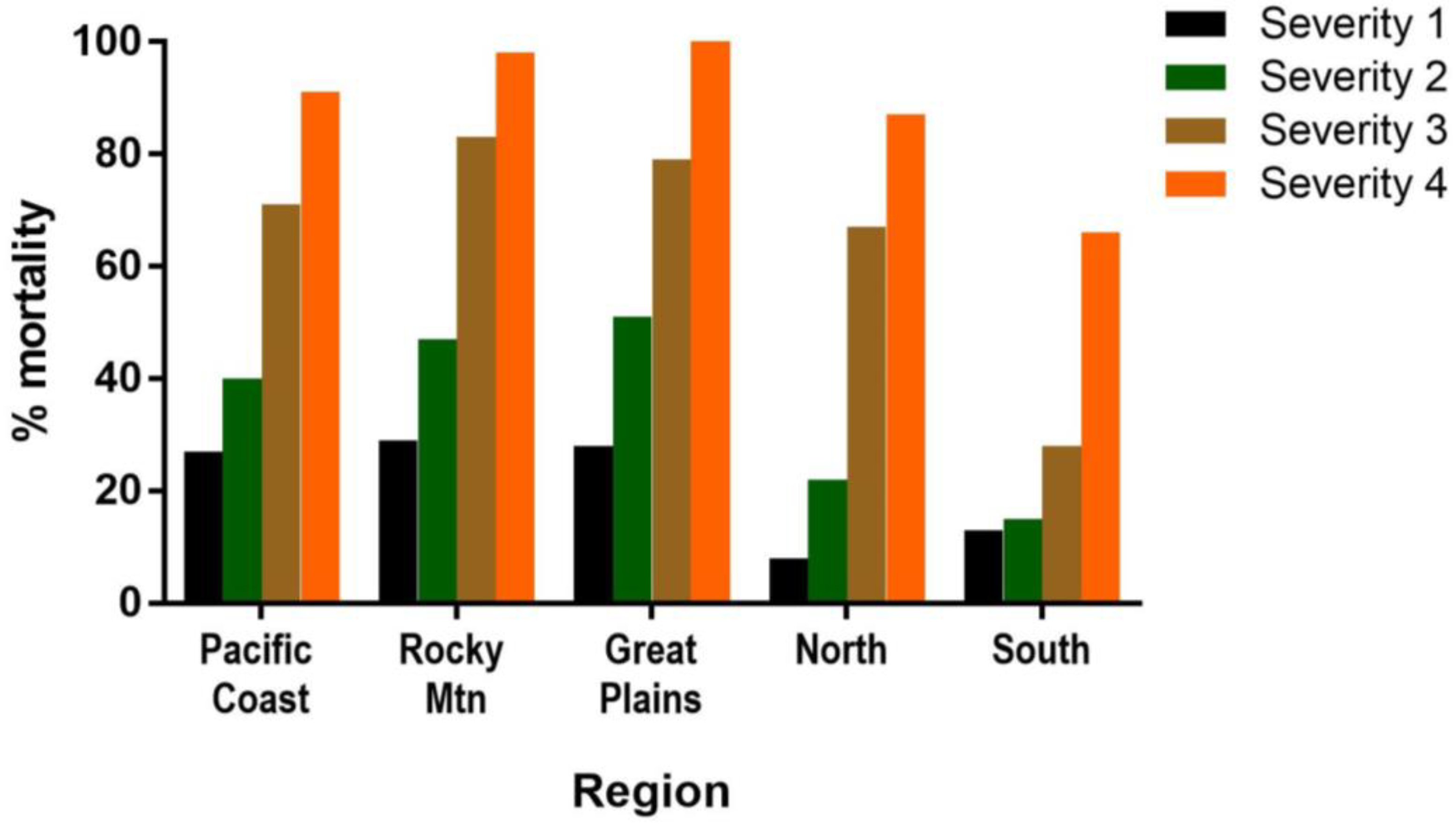
3.4. Effect of Burn Severity and the Elapsed Interval since Fire on Indicator Sensitivity

We illustrate the joint effects of burn severity and the elapsed time between the MTBS fire and the subsequent plot visit on the sensitivity of indicators (Figure 3, Figure 4 and Figure 5). Note that classifications vary (from chart to chart) because Eastern fires have very few severity class 4 fires, and the remeasurement interval is longer for most Western and Great Plains fires. In general, the greater the severity, the greater the rate of correct detection, and similarly, the more recent fires are correctly detected at higher rates. These effects are apparent for most indicators over most regions, but they are least consistent for the tree damage indicator. Rates approach maximum with increasing severity or decreasing time more rapidly in the West. All indicators on the Pacific Coast and Rocky Mountains show the clearest joint effect.

3.5. Forest Inventory Plot Locations

To generally assess the importance of exact plot locations on the intersections of inventory plots with MTBS burn perimeters, we determined the relative rates of intersection based on the publicly available altered locations. Specific identities of the pairs (i.e., plots and perimeters) were sometimes different, but 81 percent of the pairs were also identified through the publicly available plot locations (Table 5). Regionally, rates were between 67 and 92 percent. In addition to affecting intersections, location information also affects MTBS burn severity assigned at plot locations. For this comparison, we limited the set of intersections to those plots identically identified via both exact and altered locations (i.e., column-1 81 percent over CONUS). Overall, only 51 percent of these plots were associated with the same burn severity; regional values were between 44 and 63 percent of plots retaining the identical severity class based on either location source (Table 5).

4. Discussion

An important measure of the effectiveness of the plot-level fire indicators is how well they correspond to independent fire data [35,36], such as spatial and temporal intersection with the MTBS or MODIS burn perimeters (Table 2, Tables S1 and S2). Sensitivity to fire varies among indicators and over regions. Western fires are most readily identified (highest rates), and forest fires in the South have the lowest sensitivity for indicators. Western forest fires included a higher proportion of high burn severities, which may contribute to making them most apparent. The lower sensitivity in the South may be related to relatively rapid regrowth, or re-greening, after the generally lower severity fires. However, tracking post-fire stand change is outside of the scope here. Overall, site appearance from the condition table’s disturbance codes is the single indicator that is most sensitive to fires across all regions. Combining indicators increases sensitivity because there is no one indicator that identifies all the apparent MTBS forest fires. This suggests that there is value in incorporating all three indicators in any search for recent fires.
Our purpose here is to describe general trends in the sensitivity of fire indicators to label forest plots as recently burned. Spatial fire data, such as the MTBS records, are not exhaustive lists of fires, and very many additional FIA forest inventory plots are affected by fire beyond those linked to the MTBS. This analysis includes a limited set of plots and similarly limited independent fire occurrence data. The indicators provide a means of extracting plot data focused on stand-level processes relative to fire [19,37,38]. Because of statistical considerations related to inventory design, the number of plots identified as experiencing a recent fire cannot be considered proportional to the area affected by fire, and this approach of identifying fire-affected plots should not be used as a step toward estimating the area of forest land affected by fire or developing a comprehensive estimate of fire-related greenhouse gas emissions [25,39]. Also, note that while we are comparing the performance of the different indicators in detecting plots recently affected by fire, this assessment is in relation to the MTBS burn perimeter data. This study was not designed to evaluate specific FIA disturbance indicators beyond the overlay with MTBS perimeters.
Each of these FIADB-based fire indicators clearly allows for visible fire effects on plots below the thresholds for populating these fields. The condition table disturbance codes require minimums for the size of the area and the number of trees affected. With the tree-based indicators, lower severity fires may not necessarily produce tree mortality (i.e., in greater than 12.7 cm d.b.h trees) or live tree damage over 20 percent of the affected area. A less-than-distinct lower threshold for fire is also characteristic of the MTBS burn perimeter severity classifications. The unburned-to-low classification (burn severity 1) is necessarily somewhat ambiguous with respect to past fires in that it includes burn perimeter areas that are unburned, burned with minimal visible effect, or burned followed by rapid recovery [28]. As noted in Methods, we omitted the lower-end gray areas for Table 2 as compared to Table S1, which included severity class 1. However, we retained all four of the MTBS severity classes in summaries of frequency (Table 4) or number of plot-perimeter intersections (Table 5). Note that MODIS data do not include comparable fire classification information.
The lowest MTBS burn severity—the unburned-to-low classification—does not make it possible to delineate unburned islands within the scope of this analysis [28,40,41,42]. While these areas within forest fires can be important for detecting or summarizing the effects of fires, a consequence of this analysis is that we are not able to confidently assign a “no fire” label at plot-perimeter intersections. This is the primary reason for not attempting to include a specificity assessment with these results. In addition to the possibility of unburned islands, the 15 percent of forest inventory plots intersecting MTBS perimeters but failing to detect fire through any of the three indicators may have been the result of fire effects visible on the plot yet below indicator thresholds (for populating fields). The thresholds are likely set because of the difficulty in collecting the more minor burns with certainty and consistency. This suggests that smaller or low-impact fires, which may include many prescribed fires, are underrepresented in the plot records.
We defined sensitivity (e.g., for Table 2) as based on the plot-perimeter intersection (spatially and temporally) and confidence of fire at that point. In addition to the severity and elapsed time between fire and inventory plot data collection, other details of the plot-perimeter intersection can affect accuracy in quantifying sensitivity. For example, in some cases there may be multiple fires recorded within the inventory plot remeasurement interval. In cases of multiple burns within an interval, we included the most recent fire to determine the elapsed time since the burn for the analysis. Additionally, the cumulative effect of repeat fires may reinforce characteristics key to indicators and thus increase the rate of detection. Multiple fires during the remeasurement interval can occur anywhere in CONUS, but they are most common in the South. The accuracy of fire location relative to inventory plot is likely different between MTBS and MODIS records. Sensitivities within the MODIS perimeters (Table S2) are consistently slightly lower than those from the MTBS perimeters (Table S1 or Table 2). The algorithms for allocating pixels as burned areas differ between the two sources [15,27], but each is based on recognizing fire effects within a pixel but not necessarily any distribution of fire across the pixel. Based on geometry alone, the 270-fold greater area of a MODIS pixel (500 m) relative to MTBS (30 m) creates greater potential for plot and fire to not align. This may affect the differences in rates. Explicitly addressing these two issues to increase accuracy is beyond the scope of this work, and we believe that it would produce minor changes in the rates (in Table 2, Tables S1 and S2) but not change the essential results we present.
Indicators were independently evaluated at the time of plot data collection, each according to separate criteria such as mortality or live tree damage, and the different criteria suggest that there is a potential that the indicators “see” slightly different sets of fires according to characteristics or scale [18]. Despite the different bases for flagging a fire, they are all aimed at indicating a recent fire on the plot. Considering these differences, one purpose for the summaries for Table 1 is to determine if any indicator is effectively dependent on, or nested within, another indicator in a region. One specific scenario for such a possible dependence is fires that result in mortality of 12.7 cm (5-inch) d.b.h., or larger trees (i.e., the tree mortality indicator) might also be extensive enough (whatever the severity class) to appear in the other indicators as well, particularly site appearance. However, plots with fire mortality indicators failed to also include site appearance indicators of fire on 37 and 27 percent of plots for West and East respectively (from Table 1 data). While this quick informal analysis does not rule out any sort of dependence, it does suggest that the indicators are, in some cases, detecting unique fires. Each of the five regions included at least one or more plots (indicating fires) representing each of the seven possible combinations of the three indicators (i.e., individually, in pairs, or jointly by all three).
Results did suggest a general combined effect of severity and elapsed time. The pattern of relative success of the indicators in identifying forest fires shown in Table 2 (e.g., site appearance versus tree in the South) is apparent in Figure 3, Figure 4 and Figure 5, but here, the possible joint effects of burn severity and the elapsed interval are indicated for some regions. The patterns are clearest in the Pacific Coast, Rocky Mountains, and South regions, where fires are much more numerous than in the Great Plains or North. The consistent pattern of increased successful identification with increasing burn severity is seen for most regions and indicators. The notable exception is in the tree damage codes at moderate to high severity, particularly in the West. The decrease in the rate of indicating fires is probably because there are very few surviving trees in high-severity fires, and the tree damage codes only apply to live trees.
The effects of fires are variable, and the visible effects, or fire scars, may fade at different rates depending on fire and site characteristics [43,44]. Shaw et al. [19] noted that regrowth, as an increase in basal area, was not well correlated with lower burn severity plots. In most cases, an increased interval between fire and plot visit leads to lower detection rates [45,46,47]. Following lower severity burns, rates of regrowth, particularly herbaceous vegetation, are more rapid in the East relative to most of the West, and this is also related to when typical fire season is located within the year [29,48]. This is a broad generalization, and there are exceptions, such as the split of the Pacific Coast region with a generally wetter west side and a more arid east side. Regrowth provides a possible explanation for the time effect on the site appearance and tree damage indicators. A possible mechanism for the slight decrease in tree mortality fire identification with age may be falling standing dead trees over the years since the fire.
Regional characteristics of forest fires (Table 4) are based on the MTBS burn severity images. Severity classifications are most generally post-fire approaches for comparing the effects of fires across sites or forest stands [49,50]. The MTBS-specific severities we use here qualitatively conform with other severity characterizations employed for fire-related research, which assign impact classes per unit area [15,49,50]. Some minor modifications to the MTBS methods or data availability over the years of fire data accumulation may affect some uses of the data [29,41]. The severity data are widely used successfully over time [42], and our use here is to broadly sort relative levels of fire effect (i.e., “more severe” versus “less severe”). However, note that we do not link the MTBS severity classes to other published severity levels. Similarly, we do not associate severity class with any of the indicators beyond summarizing correct fire identification.
While intersecting the locations of forest inventory plots with MTBS burn perimeters identifies plots in burned areas, associating fire indicators with severity requires consistent severity labels at each location. Within the scope of this analysis, we wanted the single best representation of whole-class values rather than a continuous severity statistic. Tree mortality on these plots (Figure 2) was consistent with the integer severities we identified, giving us some confidence in the approach. This consistent allocation of severity to plots made possible the better resolution of sensitivity of Table 2 relative to Table S1.
The difference in the source of plot locations (i.e., exact versus altered [16]) does affect two aspects of this analysis. First, a repeat of the intersection calculations, such as for Table 2, would show reduced accuracy in determining the sensitivity of indicators. This is based on the reduced accuracy in identifying plot-perimeter pairs (Table 5). Secondly, altered plot locations result in different arrays of severity pixel values from the MTBS severity images. Given the fact that all plot locations are altered, then essentially all plots are located in a different set of 9 pixels in comparison with the exact locations. Despite this complete relocation, roughly half of the plots retain the same severity label between the exact and altered locations (i.e., the mode of the surrounding nine-cell severities). This is probably related to locally consistent burns within a fire perimeter, which we saw in preliminary analysis. Before selecting the nine-cell grid as representative of the plot locations, we also summarized pixels surrounding plot locations up to an 81-cell grid and randomly selected nine-cell grids sampled from within the 81 cells were very consistent in resolving to the same severity (most, but not all the time). Note that while these spatial plot location considerations affect apparent sensitivities, actual indicator performance is consistent with results in Table 2.
This basic approach of evaluating inventory-based site indicators according to separate spatial data can be generalized to other disturbances or other national forest inventories. While plot designs and data collection methods vary, a few examples of nations where forest inventory programs collect data relating to disturbance and plot and tree damage include Canada, Spain, and Switzerland [21,51,52]. The MODIS burned area product and other remote sensing products are available globally, and Canada and Spain, along with other nations, maintain databases containing information on the number of wildfires and areas burned. This suggests that the general approach of using variables in existing national forest inventory databases as indicators to identify plots affected by fire is a workable method to allow the assessment of fire impacts without the need for additional field data collection.

5. Conclusions

Each of the three inventory-plot-based indicators is sensitive to most of the recent fires identified by the intersection of FIA and MTBS data. The three fire indicators capture slightly different sets of past fires, which means that some fires are uniquely identified by only one of the indicators. This effect is regionally different. Combining all indicators is the best approach for identifying the greatest number of inventory plots with recent fires. Although this study explicitly tested plot and tree-level indicators related to a recent fire, the results suggest that this method could be useful for other disturbances (especially where independent spatial data are available), such as insect and disease outbreaks or hurricane damage. This general approach should also be feasible in any nation or region where forest inventory programs collect data that include information on disturbance damage on plots, which can be combined with separate fire or disturbance layers.

Supplementary Materials

The following supporting information can be downloaded at https://www.mdpi.com/article/10.3390/f15071264/s1, Figure S1: Layout and dimensions of FIA plots. Figure S2: Example from Washington State, USA, showing overlay of FIA plots over MODIS polygons and MTBS burn perimeter. Table S1: Percentage of inventory plots intersecting a MTBS burn perimeter where fire indicators correctly identified a recent fire. Table S2: Percentage of inventory plots intersecting a MODIS burn perimeter where fire indicators correctly identified a recent fire. Table S3: Regionally summarized common start dates for MTBS burns identified as including forest fire from 2001–2020 records.

Author Contributions

Conceptualization, J.E.S. and C.M.H.; methodology, J.E.S.; software, J.E.S.; validation, J.E.S. and C.M.H.; writing—original draft preparation, J.E.S. and C.M.H.; writing—review and editing, J.E.S. and C.M.H. All authors have read and agreed to the published version of the manuscript.

Funding

This research received no external funding.

Data Availability Statement

Data will be made available on request.

Acknowledgments

We thank the reviewers for their feedback, which improved the manuscript, and we gratefully acknowledge the work of the FIA field crews and data managers.

Conflicts of Interest

The authors declare no conflicts of interest.

References

  1. Cattau, M.E.; Wessman, C.; Mahood, A.; Balch, J.K. Anthropogenic and lightning-started fires are becoming larger and more frequent over a longer season length in the U.S.A. Glob. Ecol. Biogeogr. 2020, 29, 668–681. [Google Scholar] [CrossRef]
  2. Dennison, P.E.; Brewer, S.C.; Arnold, J.D.; Moritz, M.A. Large wildfire trends in the western United States, 1984–2011. Geophys. Res. Lett. 2014, 41, 2928–2933. [Google Scholar] [CrossRef]
  3. Westerling, A.L.R. Increasing western US forest wildfire activity: Sensitivity to changes in the timing of spring. Philos. Trans. R. Soc. B 2016, 371, 20150178. [Google Scholar] [CrossRef] [PubMed]
  4. Yang, J.; Tian, H.; Tao, B.; Ren, W.; Pan, S.; Liu, Y.; Wang, Y. A growing importance of large fires in conterminous United States during 1984–2012. J. Geophys. Res. Biogeosciences 2015, 120, 2625–2640. [Google Scholar] [CrossRef]
  5. Barbero, R.; Abatzoglou, J.T.; Larkin, N.K.; Kolden, C.A.; Stocks, B. Climate change presents increased potential for very large fires in the contiguous United States. Int. J. Wildland Fire 2015, 24, 892–899. [Google Scholar] [CrossRef]
  6. Halofsky, J.E.; Peterson, D.L.; Harvey, B.J. Changing wildfire, changing forests: The effects of climate change on fire regimes and vegetation in the Pacific Northwest, USA. Fire Ecol. 2020, 16, 4. [Google Scholar] [CrossRef]
  7. Vose, J.M.; Peterson, D.L.; Domke, G.M.; Fettig, C.J.; Joyce, L.A.; Keane, R.E.; Luce, C.H.; Prestemon, J.P.; Band, L.E.; Clark, J.S.; et al. Impacts, Risks, and Adaptation in the United States: Fourth National Climate Assessment, Volume II; Reidmiller, D.R., Avery, C.W., Easterling, D.R., Kunkel, K.E., Lewis, K.L.M., Maycock, T.K., Stewart, B.C., Eds.; U.S. Global Change Research Program: Washington, DC, USA, 2018; pp. 232–267. [CrossRef]
  8. Hohner, A.K.; Rhoades, C.C.; Wilkerson, P.; Rosario-Ortiz, F.L. Wildfires alter forest watersheds and threaten drinking water quality. Acc. Chem. Res. 2019, 52, 1234–1244. [Google Scholar] [CrossRef] [PubMed]
  9. Smith, H.G.; Sheridan, G.J.; Lane, P.N.J.; Nyman, P.; Haydon, S. Wildfire effects on water quality in forest catchments: A review with implications for water supply. J. Hydrol. 2011, 396, 170–192. [Google Scholar] [CrossRef]
  10. Agbeshie, A.A.; Abugre, S.; Atta-Darkwa, T.; Awuah, R. A review of the effects of forest fire on soil properties. J. For. Res. 2022, 33, 1419–1441. [Google Scholar] [CrossRef]
  11. Stevens-Rumann, C.S.; Morgan, P. Tree regeneration following wildfires in the western US: A review. Fire Ecol. 2019, 15, 15. [Google Scholar] [CrossRef]
  12. Rocca, M.E.; Brown, P.B.; MacDonald, L.H.; Carrico, C.M. Climate change impacts on fire regimes and key ecosystem services in Rocky Mountain forests. For. Ecol. Manag. 2014, 327, 290–305. [Google Scholar] [CrossRef]
  13. Roces-Díaz, J.V.; Santín, C.; Martínez-Vilalta, J.; Doerr, S.H. A global synthesis of fire effects on ecosystem services of forests and woodlands. Front. Ecol. Environ. 2022, 20, 170–178. [Google Scholar] [CrossRef]
  14. Sánchez, J.J.; Marcos-Martinez, R.; Srivastava, L.; Soonsawad, N. Valuing the impacts of forest disturbances on ecosystem services: An examination of recreation and climate regulation services in U.S. national forests. Trees For. People 2021, 5, 100123. [Google Scholar] [CrossRef]
  15. Eidenshink, J.; Schwind, B.; Brewer, K.; Zhu, Z.L.; Quayle, B.; Howard, S. A project for monitoring trends in burn severity. Fire Ecol. 2007, 3, 3–21. [Google Scholar] [CrossRef]
  16. Burrill, E.A.; DiTommaso, A.M.; Turner, J.A.; Pugh, S.A.; Menlove, J.; Christensen, G.; Perry, C.J.; Conkling, B.L. The Forest Inventory and Analysis Database: Database Description and User Guide Version 9.1 for Phase 2; U.S. Department of Agriculture, Forest Service: Washington, DC, USA, 2023; 1066p. Available online: https://www.fia.fs.usda.gov/library/database-documentation/index (accessed on 8 November 2023).
  17. USDA Forest Service 2024. U.S. Department of Agriculture, Forest Service. Forest Inventory and Analysis National Program. USDA Forest Service, Washington, DC, USA. Available online: https://www.fs.usda.gov/research/programs/fia (accessed on 26 April 2024).
  18. Fitts, L.A.; Domke, G.M.; Russell, M.B. Comparing methods that quantify forest disturbances in the United States’ national forest inventory. Environ. Monit. Assess. 2022, 194, 304. [Google Scholar] [CrossRef] [PubMed]
  19. Shaw, J.D.; Goeking, S.A.; Menlove, J.; Werstak, C.E. Assessment of fire effects based on forest inventory and analysis data and a long-term fire mapping data set. J. For. 2017, 115, 258–269. [Google Scholar] [CrossRef]
  20. Woolman, A.M.; Coop, J.D.; Shaw, J.D.; DeMarco, J. Extent of recent fire-induced losses of ponderosa pine forests of Arizona and New Mexico, USA. For. Ecol. Manag. 2022, 520, 120381. [Google Scholar] [CrossRef]
  21. Schroeder, T.A.; Healey, S.P.; Moisen, G.G.; Frescinoa, T.S.; Cohen, W.B.; Huang, C.; Kennedy, R.E.; Yang, Z. Improving estimates of forest disturbance by combining observations from Landsat time series with U.S. Forest Service Forest Inventory and Analysis data. Remote Sens. Environ. 2014, 154, 61–73. [Google Scholar] [CrossRef]
  22. Hoover, C.M.; Bartig, J.L.; Bogaczyk, B.; Breeden, C.; Iverson, L.R.; Prout, L.; Sheffield, R.M. Forest Inventory and Analysis Data in Action: Examples from Eastern National Forests. Trees For. People 2022, 7, 100178. [Google Scholar] [CrossRef]
  23. Fei, S.; Morin, R.S.; Oswalt, C.M.; Liebhold, A.M. Biomass losses resulting from insect and disease invasions in US forests. PNAS 2019, 116, 17371–17376. [Google Scholar] [CrossRef]
  24. Canada’s National Forest Inventory—National Standards for Ground Plots Data Dictionary, Version 5.2.3. Available online: http://nfi.nfis.org (accessed on 7 June 2024).
  25. Westfall, J.A.; Coulston, J.W.; Moisen, G.G.; Andersen, H.E. Sampling and Estimation Documentation for the Enhanced Forest Inventory and Analysis Program; General Technical Report NRS-GTR-207; Department of Agriculture, Forest Service, Northern Research Station: Madison, WI, USA, 2022; 129p. [CrossRef]
  26. USDA Forest Service. Nationwide Forest Inventory Field Guide; USDA Forest Service: Washington, DC, USA, 2024. Available online: https://www.fs.usda.gov/research/understory/nationwide-forest-inventory-field-guide (accessed on 15 May 2024).
  27. Giglio, L.; Boschetti, L.; Roy, D.P.; Humber, M.L.; Justice, C.O. The Collection 6 MODIS burned area mapping algorithm and product. Remote Sens. Environ. 2018, 217, 72–85. [Google Scholar] [CrossRef] [PubMed]
  28. MTBS. Monitoring Trend in Burn Severity. Website and Data. Available online: https://www.mtbs.gov/ (accessed on 15 August 2023).
  29. Picotte, J.J.; Bhattarai, K.; Howard, D.; Lecker, J.; Epting, J.; Quayle, B.; Benson, N.; Nelson, K. Changes to the Monitoring Trends in Burn Severity program mapping production procedures and data products. Fire Ecol. 2020, 16, 16. [Google Scholar] [CrossRef]
  30. French, N.H.F.; McKenzie, D.; Erickson, T.; Koziol, B.; Billmire, M.; Endsley, K.A.; Yager Scheinerman, N.K.; Jenkins, L.; Miller, M.E.; Ottmar, R.; et al. Modeling regional-scale wildland fire emissions with the Wildland Fire Emissions Information System. Earth Interact. 2014, 18, 1–26. [Google Scholar] [CrossRef]
  31. WFEIS. Wildland Fire Emissions Inventory System, Calculator. 2023. Available online: https://wfeis.mtri.org/calculator (accessed on 30 June 2023).
  32. Dewitz, J.; U.S. Geological Survey. National Land Cover Database (NLCD) 2019 Products (Ver. 2.0, June 2021): U.S. Geological Survey. Land Cover Data Online Release. Available online: https://doi.org/10.5066/P9KZCM54 (accessed on 10 July 2024).
  33. NLCD. National Land Cover Database: NLCD Land Cover with additional Forest Transition Classes. 2023. Available online: https://www.mrlc.gov/nlcd-2021-science-research-products (accessed on 10 July 2023).
  34. Pelletier, F.; Eskelson, B.N.I.; Monleon, V.J.; Tseng, Y.C. Using Landsat Imagery to Assess Burn Severity of National Forest Inventory Plots. Remote Sens. 2021, 13, 1935. [Google Scholar] [CrossRef]
  35. Odion, D.C.; Hanson, C.T.; Baker, W.L.; DellaSala, D.A.; Williams, M.A. Areas of Agreement and Disagreement Regarding Ponderosa Pine and Mixed Conifer Forest Fire Regimes: A Dialogue with Stevens et al. PLoS ONE 2016, 11, e0154579. [Google Scholar] [CrossRef] [PubMed]
  36. Whittier, T.R.; Gray, A.N. Tree mortality based fire severity classification for forest inventories: A Pacific Northwest national forests example. For. Ecol. Manag. 2016, 359, 199–209. [Google Scholar] [CrossRef]
  37. Collins, B.M.; Roller, B. Early forest dynamics in stand-replacing fire patches in the northern Sierra Nevada, California, USA. Landsc. Ecol. 2013, 28, 1801–1813. [Google Scholar] [CrossRef]
  38. Ojha, S.K.; Naka, K.; Dimov, L.D. Assessment of Disturbances across Forest Inventory Plots in the Southeastern United States for the Period 1995–2018. For. Sci. 2020, 66, 242–255. [Google Scholar] [CrossRef]
  39. Yu, Y.; Saatchi, S.; Domke, G.M.; Walters, B.; Woodall, C.; Ganguly, S.; Li, S.; Kalia, S.; Park, T.; Nemani, R.; et al. Making the US national forest inventory spatially contiguous and temporally consistent. Environ. Res. Lett. 2022, 17, 065002. [Google Scholar] [CrossRef]
  40. Kolden, C.A.; Smith, A.M.; Abatzoglou, J.T. Limitations and utilisation of Monitoring Trends in Burn Severity products for assessing wildfire severity in the USA. Int. J. Wildland Fire 2015, 24, 1023–1028. [Google Scholar] [CrossRef]
  41. Kolden, C.A.; Lutz, J.A.; Key, C.H.; Kane, J.T.; van Wagtendonk, J.W. Mapped versus actual burned area within wildfire perimeters: Characterizing the unburned. For. Ecol. Manag. 2012, 286, 38–47. [Google Scholar] [CrossRef]
  42. Picotte, J.J.; Peterson, B.; Meier, G.; Howard, S.M. 1984–2010 trends in fire burn severity and area for the conterminous US. Int. J. Wildland Fire 2016, 25, 413–420. [Google Scholar] [CrossRef]
  43. Baker, W.L.; Ehle, D. Uncertainty in surface-fire history: The case of ponderosa pine forests in the western United States. Can. J. For. Res. 2001, 31, 1205–1226. [Google Scholar] [CrossRef]
  44. Marlon, J.R.; Bartlein, P.J.; Gavin, D.G.; Long, C.J.; Anderson, R.S.; Briles, C.E.; Brown, K.J.; Colombaroli, D.; Hallett, D.J.; Power, M.J.; et al. Long-term perspective on wildfires in the western USA. Proc. Natl. Acad. Sci. USA 2012, 109, E535–E543. [Google Scholar] [CrossRef] [PubMed]
  45. Bright, B.C.; Hudak, A.T.; Kennedy, R.E.; Braaten, J.D.; Khalyani, A.H. Examining post-fire vegetation recovery with Landsat time series analysis in three western North American forest types. Fire Ecol. 2019, 15, 8. [Google Scholar] [CrossRef]
  46. Rother, D.E.; De Sales, F.; Stow, D.; McFadden, J. Impacts of burn severity on short-term postfire vegetation recovery, surface albedo, and land surface temperature in California. PLoS ONE 2022, 17, 11. [Google Scholar] [CrossRef]
  47. Yang, J.; Pan, S.; Dangal, S.; Zhang, B.; Wang, S.; Tian, H. Continental-scale quantification of post-fire vegetation greenness recovery in temperate and boreal North America. Remote Sens. Environ. 2017, 199, 277–290. [Google Scholar] [CrossRef]
  48. Tangney, R.; Paroissien, R.; Le Breton, T.D.; Thomsen, A.; Doyle, C.A.T.; Ondik, M.; Miller, R.G.; Miller, B.P.; Ooi, M.K.J. Success of post-fire plant recovery strategies varies with shifting fire seasonality. Commun. Earth Environ. 2022, 3, 126. [Google Scholar] [CrossRef]
  49. Han, D.; Di, X.; Yang, G.; Sun, L.; Weng, Y. Quantifying fire severity: A brief review and recommendations for improvement. Ecosyst. Health Sustain. 2021, 7, 1973346. [Google Scholar] [CrossRef]
  50. Keeley, J.E. Fire intensity, fire severity and burn severity: A brief review and suggested usage. Int. J. Wildland Fire 2009, 18, 116–126. [Google Scholar] [CrossRef]
  51. Ministerio Para La Transición Ecológica Y El Reto Demográfico. Fourth Forest Inventory (IFN4) Description of the Database Codes Field Data. Available online: https://www.miteco.gob.es/content/dam/miteco/es/biodiversidad/temas/inventarios-nacionales/ifn/ifn4/documentador_ifn4_campo_tcm30-536595.pdf (accessed on 10 June 2024).
  52. Keller, M. (Ed.) Swiss National Forest Inventory. Manual of the Field Survey 2004–2007. 2011; Available online: https://www.dora.lib4ri.ch/wsl/islandora/object/wsl:10498 (accessed on 10 June 2024).
Figure 1. Regions as defined for this analysis. Pacific Coast, Rocky Mountains, and Great Plains are considered west, with North and South as east.
Forests 15 01264 g001
Figure 2. Percent mortality of tally trees according to the burn severity class assigned to the intersection of inventory plot and MTBS burn perimeter (from inventory years 2013–2019).
Forests 15 01264 g002
Figure 3. Effects of burn severity and time on the frequency of detecting an MTBS fire in the Pacific Coast and Rocky Mountains regions. Panels summarize the effect of elapsed time intervals (between fire and subsequent plot visit) for bins of 0–2 years (a,d), 3–5 years (b,e), and 6–8 years (c,f). Groups of bars represent combined (‘any’) and the individual indicators. Bars represent burn severities 2 through 4 (low to high).
Forests 15 01264 g003
Figure 4. Effects of burn severity and time on the frequency of detecting an MTBS fire in the South region. Panels summarize the effect of elapsed time intervals (between fire and subsequent plot visit) for bins of 0–2 years (a) and 3–5 years (b). Groups of bars represent combined (“any”) and the individual indicators. Bars represent burn severities 2 through 3 (low to moderate).
Forests 15 01264 g004
Figure 5. Effects of burn severity and time on the frequency of detecting an MTBS fire in the Great Plains and North regions. Panels summarize the effect of elapsed time intervals (between fire and subsequent plot visit) for bins of 0–2 years (a,d), 3–5 years (b,e), and 6–8 years (c). Groups of bars represent combined (“any”) and the individual indicators. Bars represent burn severities 2 through 3 (low to moderate).
Forests 15 01264 g005
Table 1. Percentages of forest inventory plots that include indicators of recent fire, as summarized from the inventory years 2013–2019. The counts of “Plots with forest” are annual averages over the 7-year interval.
RegionAny
Indicator
Both Site and TreeSite
Appearance
Any TreeTree
Mortality
Tree
Damage
Plots with Forest
Percentage of plots (n)n
Pacific Coast13.8 (298)6.2 (134)7.1 (154)12.8 (278)6.8 (147)9.9 (214)2160
Rocky Mountains8.7 (223)5.0 (129)5.5 (141)8.2 (211)6.6 (170)3.4 (87)2575
Great Plains6.1 (64)2.9 (31)4.4 (46)4.6 (49)2.6 (27)3.2 (34)1053
North1.0 (63)0.4 (25)0.5 (35)0.8 (53)0.3 (23)0.6 (42)6523
South8.6 (626)3.4 (244)7.6 (548)4.4 (322)2.5 (179)3.1 (224)7259
Table 2. Percentage of inventory plots intersecting an MTBS burn perimeter where fire indicators correctly identified a recent fire. The set of plots on burn perimeters is limited to burn severity classes 2 through 4 (low to high) at the plot location. Plots on forest land are from inventory years 2013–2019, and the last column is the average annual number of plots with forest.
RegionAny
Indicator
Site
Appearance
Any TreeTree
Mortality
Tree
Damage
Forest Plots within MTBS Perimeter
Percentage of plots (n)n per year
Pacific Coast96 (105)94 (102)89 (97)83 (90)51 (56)109
Rocky Mountains89 (105)79 (93)86 (102)84 (99)26 (30)118
Great Plains80 (25)75 (23)60 (18)45 (14)38 (12)31
North83 (8)75 (7)72 (7)52 (5)48 (4)9
South79 (99)72 (91)50 (63)28 (36)38 (49)127
Table 3. Percentage of inventory plots intersecting an MTBS burn perimeter where fire indicators correctly identified a recent fire, according to burn severity (i.e., sensitivity by severity). From inventory years 2013–2019.
RegionSeverity Classn per YearSite
Appearance
Tree
Mortality
Tree
Damage
Mean percentage identified
Pacific Coast248.4927970
333.0958454
427.1978916
Rocky Mountains258.3697435
335.9879125
423.793976
Great Plains223.0683736
37.1946846
40.6100750
North26.3684157
32.3886931
40.610010025
South2110.9712638
314.3793945
41.4706010
Table 4. Regional patterns of burn severity of forest fires within MTBS burn perimeters over 20 years (2001–2020) of records. Based on MTBS burn severity coinciding with NLCD forest cover (pixel pairs).
RegionUnburned to Low Severity (Class 1)Low Severity (Class 2)Moderate
Severity
(Class 3)
High
Severity
(Class 4)
Fires Entirely Severity 1 or 2Fires
without
Severity 4
Percentage of total burned forest areaPercentage of fires
Pacific Coast223923161126
Rocky Mountains224124141333
Great Plains4648518192
North2467725988
South2071915388
Table 5. Effect of the FIADB-based altered plot locations on correctly identifying intersections of inventory plots with MTBS burn perimeters. Additionally, the percentage of the column-1 plot-perimeter combinations that also correctly assign identical MTBS burn severities to the plot. Note: The total number of actual-location-based intersections is the 3664 underlying Table 2.
RegionPlot-Perimeter Pairs Identified by
Altered Plot Locations
From Column 1, Plots Also Correctly
Assigned Burn Severity
Percentage
Pacific Coast9250
Rocky Mountains8744
Great Plains7963
North6754
South6757
Disclaimer/Publisher’s Note: The statements, opinions and data contained in all publications are solely those of the individual author(s) and contributor(s) and not of MDPI and/or the editor(s). MDPI and/or the editor(s) disclaim responsibility for any injury to people or property resulting from any ideas, methods, instructions or products referred to in the content.

