Tree Height Estimation of Chinese Fir Forests Based on Geographically Weighted Regression and Forest Survey Data

Abstract

Estimating tree height at the national to regional scale is crucial for assessing forest health and forest carbon storage and understanding forest ecosystem processes. It also aids in formulating forest management and restoration policies to mitigate global climate change. Extensive ground-survey data offer a valuable resource for estimating tree height. In tree height estimation modeling, a few comparative studies have examined the effectiveness of global-based versus local-based models, and the spatial heterogeneity of independent variable parameters remains insufficiently explored. This study utilized ~200,000 ground-survey data points covering the entire provincial region to compare the performance of the global-based Ordinary Least Squares (OLS) and Random Forest (RF) model, as well as local-based Geographically Weighted Regression (GWR) model, for predicting the average tree height of Chinese fir forests in Zhejiang Province China. The results showed that the GWR model outperformed both OLS and RF in terms of predictive accuracy, achieving an R-squared (R²) and adjusted R² of 0.81 and MAE and RMSE of 0.93 and 1.28, respectively. The performance indicated that the local-based GWR held advantages over global-based models, especially in revealing the spatial non-stationarity of forests. Visualization of parameter estimates across independent variables revealed spatial non-stationarity in their impact effects. In mountainous areas with dense forest coverage, the parameter estimates for average age were notably higher, whereas in forests proximate to urban areas, the parameters were comparatively lower. This study demonstrates the effectiveness of large ground-survey data and GWR in tree height estimation modeling at a provincial scale.

1. Introduction

Tree height is critical in assessing forest health [1,2] and estimating forest biomass and carbon storage [3]. It also plays a pivotal role in understanding forest ecosystems and biodiversity [4,5,6] and developing forest management policies [7,8,9,10]. Accurately quantifying tree height has always been an important task in National Forest Inventories(NFI), including the Chinese National Forest Continues Inventory and Forest Management Inventory [11,12]. In these forest survey missions, the height of each tree within fixed-size plots or forest sub-compartments is measured and recorded.

The National Forest Management Inventory (FMI), alternatively known as the Forest Resource Planning and Design Survey, is a type of direct ground survey. The data obtained from FMI are extensively used for estimating diverse forest information. For example, Ground-survey indicators, including forest origin, tree age, and dominant species from FMI data, were used to estimate forest ecological function levels [13]. FMI data with terrain factors were selected by different variable selection methods for forest stock volume estimation [14]. The sample and reference datasets were collected from FMI to predict dominant species’ commonly quantified forest variables, including canopy cover, diameter at breast height, and tree canopy height [15]. It can be concluded that FMI data serves as an important data source in forest information inversion models.

In previous studies, forest tree height estimation models utilize data from multiple sources [16,17,18,19], among which forest survey data continue to be indispensable data [15,20]. Various models have been developed to integrate multi-sources data. For instance, least squares regression was applied to estimate the global tree height using remote sensing images [21]. The performance of Artificial Neural Networks was evaluated, and three forest survey variables were used, including diameter at breast height, height at the base of the crown, and the position of the trees [22]. Machine learning models such as the Random Forest (RF) algorithm were used to develop a wall-to-wall vegetation height map of China with the vegetation height data extracted from the satellite data and various ancillary data including canopy cover information, reflectance and Leaf Area Index (LAI) data, climate data, and topographic data [23]. A neural network-guided interpolation method was developed to map large-scale tree height distribution inspired by the Third Law of Geography, which hypothesized that items with similar geographic conditions are more related [24]. According to these aforementioned studies, we can find that there are still challenges to map tree height distribution at national to regional scales accurately. When modeling spatial processes and variable relationships using various statistical learning and machine learning models, it is commonly assumed that these models are constant and location-independent. In other words, those “global” models may be limited when processes vary with spatial context.

The geographically weighted regression (GWR) model was first proposed by Brunsdon [25], inspired by Tobler’s First Law of Geography: “Everything is related to everything else, but near things are more related than distant things”. GWR is a geostatistical method allowing the relationship between independent variables and dependent variables to change locally [26]. Compared to ‘global’ regressions which assume relationships are spatially constant, GWR is a ‘local’ model to capture spatial heterogeneity and non-stationarity. GWR is proven to provide better model fit and reduced residual spatial autocorrelation and has attracted much attention in diverse fields, including land-use modeling [27] and forest ecosystem analysis [28]. In the meantime, the GWR model has been utilized in forestry applications to investigate the relationships between various forest variables and influencing factors. For instance, Forest Continues Inventory data and remote sensing data were used to predict the biomass of different vegetation types. The GWR model was constructed by combining topographical and socio-economic factors to analyze the driving factors of biomass in public welfare forests [29]. Ground-measured forest aboveground biomass (AGB) samples were collected from the Changbai Mountains in China, and the GWR model and machine learning (ML) algorithms were established and compared [30]. The comparison was made among the GWR model, Multiscale Geographically Weighted Regression (MGWR), Temporal Weighted Regression (TWR), and Geographically and Temporally Weighted Regression (GTWR), as well as the Global Ordinary Least Squares (OLS) model and Linear Mixed Model (LMM), the optimal model was selected to explore the spatiotemporal dynamics of the aboveground carbon storage in the Nature Reserve [31]. In recent years, the application of GWR models in forestry has been increasing. As a local-based model, the GWR model has the potential to provide more precise estimation results than global-based models. Moreover, the spatial non-stationarity of the independent variables has not been fully discussed.

This study utilized nearly 200,000 Forest Management Inventory data points covering the entire provincial region to construct models based on Global OLS and RF, as well as a local-based GWR model, to predict the tree height of Chinese fir forests in Zhejiang Province. The main contributions of this paper are: (1) the height of the Chinese fir forest within the scope of the entire provincial region was estimated by adopting GWR with a large amount of ground-survey data. (2) The effectiveness of global-based models and local-based models were compared and discussed (Section 3.2 and Section 4.2), and (3) the spatial heterogeneity of the parameter estimates was revealed (Section 3.4).

2. Materials and Methods

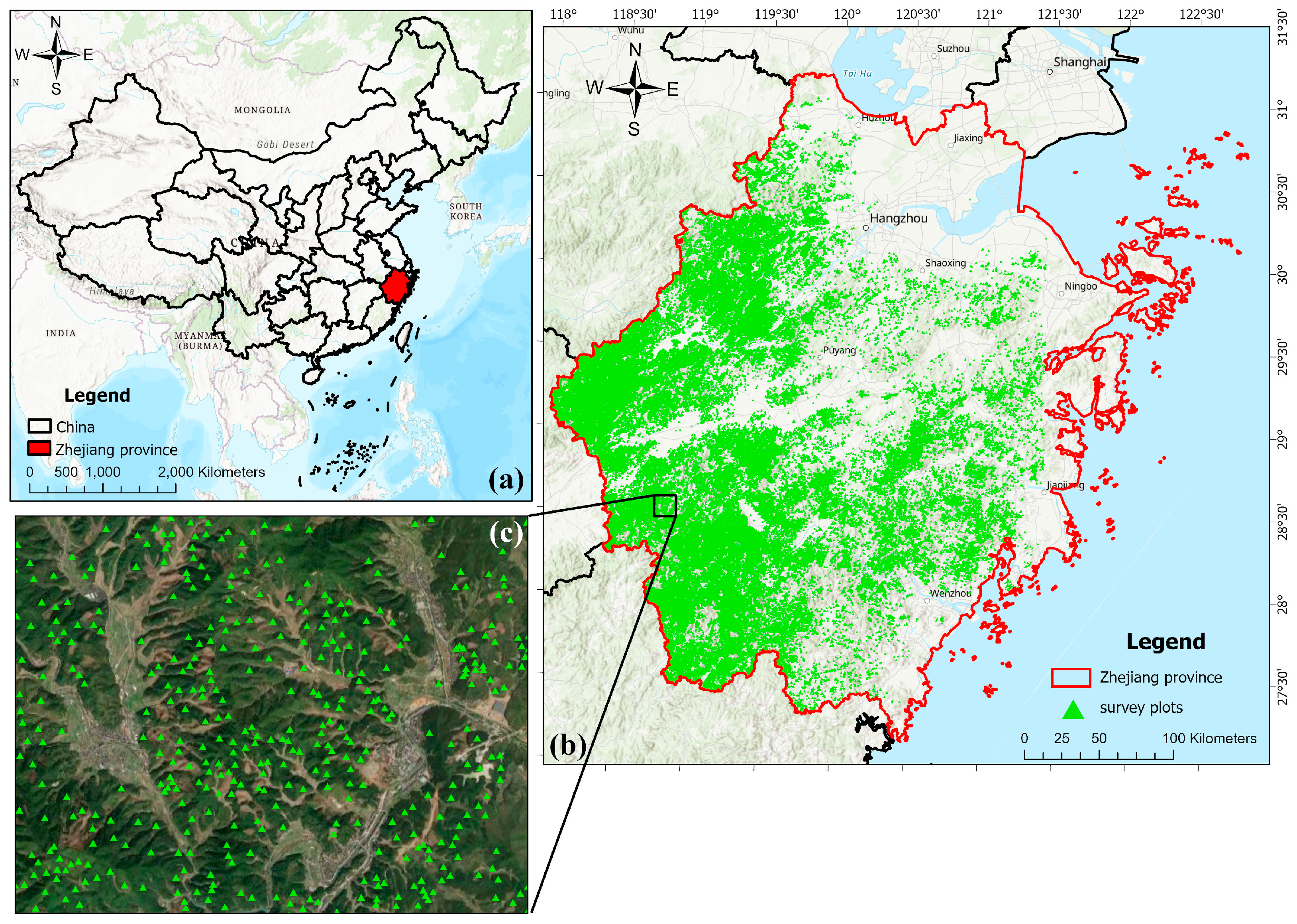
2.1. Study Area

Zhejiang Province is located on the southern wing of the Yangtze River Delta along the southeast coast of China, spanning latitudes from 27°02′ N to 31°11′ N and longitudes from 118°01′ E to 123°10′ E. The straight-line distances from east to west and from north to south in Zhejiang are both about 450 km, with a land area of 105,500 square kilometers. Situated in the central part of the subtropical zone, Zhejiang has a monsoon–humid climate characterized by moderate temperatures, distinct seasons, ample sunlight, and abundant rainfall. The average annual temperature ranges from 15 °C to 18 °C, the annual sunshine duration is between 1100 and 2200 h, and the average annual precipitation is between 1100 and 2000 mm. The map of Zhejiang Province is illustrated in Figure 1.

2.2. Forest Survey Data

The Forest Resource Planning and Design Survey Data were collected as the main FMI data. The primary objectives of this survey are to identify forest types and forest resource characteristics, forest quantities, qualities, and forest distribution and to clarify the status of forest land categories and the management characteristics of all forest land. The in-situ survey was carried out by the Zhejiang Provincial Forestry Department in 2020.

This systematic survey uses the sub-compartments as the basic unit. A sub-compartment is defined as a geographical unit that is internally consistent in its characteristics and significantly different from neighboring areas. Sub-compartments are divided by different forest categories, forest ownership, species composition, origins, age, and terrain boundaries, including ridgelines, valleys, roads, etc. Consequently, the FMI data include a comprehensive vector map of the area, composed of numerous sub-compartments. The attributes of each sub-compartment record various survey factors, including elevation, aspect, slope, soil layer thickness (SLT), humus layer thickness, forest protection grade, understory species, understory height (UH), forest structure, origin, tree species composition, average age, average tree height (TH), and other forest variables.

In our study, the sub-compartments where Chinese fir is the dominant tree species were selected first. Chinese fir (Cunninghamia lanceolata) is a primary afforestation tree species in the subtropical regions of China, accounting for approximately 25% of the area covered by man-made forests [32]. The dominant tree species is considered the principal tree species in a single sub-compartment. According to the Technical Operation Rules for FMI, a tree species is considered dominant if it constitutes a proportion greater than 65% of the growing stock volume (GSV) within a plot [33]. Some ground-based measurement variables, including elevation, slope, SLT, and humus layer thickness, were collected. The average tree height (TH) and age were determined based on the dominant tree species within a sub-compartment. Then, the data with zero or null values in tree height were removed. Consequently, 191,954 valid samples were retained for modeling.

Table 1. The FMI variables collected in this study.

No.	FMI Variables	Description
1	elevation	average elevation within sub-compartments, recorded in meters, extracted from Digital Elevation Models (DEM)
2	aspect	categorical variable with nine aspects: east, south, west, north, northeast, southeast, northwest, southwest, and no aspect
3	slope position	categorical variable with ridge, upper, middle, lower, valley, flat, and full slope
4	slope	average slope within sub-compartments, recorded in degree of angle, extracted from Digital Elevation Models (DEM)
5	SLT	average soil layer thickness within sub-compartments, recorded in centimeters
6	humus layer thickness	categorical variable, divided into thick, medium, and thin three grades, less than 2 cm is defined as thin grade, higher than 5 cm is defined as thick grade
7	site quality class	categorical variable, according to the terrain characteristics, soil, and other natural environmental factors at the location of the plot, the forest land quality was evaluated into 5 levels
8	forest protection grade	categorical variable, divided into 3 levels according to county-level forest protection planning
9	understory species	according to the vegetation type of shrub layer and herbaceous layer under the tree layer, the understory species are divided into 8 categories, including non-vegetation, grass, straw, etc.
10	UH	average height of the understory, recorded in meters
11	forest structure	categorical variable, forest structure is divided into complete structure, relatively complete structure, and simple structure according to whether it includes tree layer, underwood layer, and ground cover layer
12	origin	According to the development pattern of the stand, it is divided into two major categories and 7 subclasses
13	tree species composition	When there is only one tree species (group) in sub-compartments, only the tree name is recorded. When multiple tree species are mixed, use the ten-point method to record and write the dominant tree species first. This study took Chinese fir as the research object, so this variable was divided into two categories: pure forest and mixed forest.
14	average age	average age of dominant tree species
15	TH	average tree height of dominant species, recorded in meters

summarizes all the forest survey variables collected and utilized in this study. These variables will subsequently undergo feature selection prior to model training.

2.3. Research Framework

The workflow of this study encompasses the following steps (Figure 2): Initially, the dataset, comprising nearly 200,000 records, was randomly partitioned into a training set (80%) and a test set (20%). Subsequently, feature selection was performed using the Recursive Feature Elimination (RFE) algorithm. The refined training set was fed into both the local-based GWR model and the global-based models for training: the RF model and the OLS regression. The average tree height (TH) was designated as the dependent variable, with the remaining features serving as independent variables. Accuracy assessment and model comparison were conducted using the test dataset across the three models. Finally, a visual analysis was conducted of each feature’s parameter estimates derived from the GWR model.

2.4. Recursive Feature Elimination

Recursive Feature Elimination (RFE) is a wrapper method employed for feature selection, operating in a stepwise fashion to construct a model and discard the least significant features. The operational principle is as follows: Initially, the model is trained on all features, and the corresponding weights or coefficients for each feature are determined. Subsequently, the features are ranked according to their weights, and the one with the least weight is eliminated. These two aforementioned steps are iteratively repeated until the feature set is reduced to the desired size.

In this step, an RF regressor was adopted as the estimator, reducing the initial 14 features to the 5 most important ones. This approach allowed us to identify and retain only the most influential predictors for the model. All models utilized the same input independent variables for comparative purposes.

2.5. RF Algorithm

In our study, RF was used as a benchmark. The RF is an ensemble of multiple decision trees that incorporate random sampling, combining Breiman’s “bagging” method with random feature selection [34]. Bootstrap samples are drawn to build decision trees initially; at each split, a random subset of features determines the best division. Subsequently, trees continue to branch until they meet the stopping criteria. Finally, predictions aggregate via voting for classification or averaging for regression.

RF model includes three hyperparameters: the number of trees, the number of features randomly sampled at each split, and the maximum depth. These hyperparameters were tuned by grid search (Grid SearchCV) with Mean Squared Error evaluation through ten-fold cross-validation [35] in this study. The RF model was built using Python 3.11.7 and Scikit-Learn library.

2.6. Ordinary Least Squares

The OLS method is a fundamental approach for determining the nature of relationships among variables through linear regression modeling. In this approach, the relations between the dependent variable $y_i$ and the independent variables $x_{i1},x_{i2},x_{i3},\dots ,x_{ip}$ can be expressed as:

$$y_i={\beta }_0+\sum _{k=1}^p{\beta }_k{x}_{ik}+{ϵ}_i,i=\mathrm{1,2},\dots ,n$$

(1)

where ${\beta }_0$ is the constant coefficient of the regression, ${\beta }_1, { \beta }_2, \dots , {\beta }_p$ are the regression coefficients of the corresponding independent variables, and ${ϵ}_i$ is the error of sample $i$.

The estimates of the OLS model in matrix form are as follows:

$$\widehat{\beta }={\left(X^{T}X\right)}^{-1}{X}^{T}y$$

(2)

2.7. The Geographically Weighted Regression

The primary concern with the GWR model is its initial inability to capture the nuanced spatial variations that a global model’s coefficient estimates may fail to represent. Consequently, GWR extends the global model by allowing the regression coefficients to vary spatially, facilitating local estimations that can more accurately reflect the underlying spatial processes and variations that a single set of global coefficients might overlook. GWR can be mathematically formulated as

$$y_i={\beta }_0(u_i,v_i)+\sum _{k=1}^p{\beta }_k(u_i,v_i)x_{ik}+{ϵ}_i, i=\mathrm{1,2},\dots ,n$$

(3)

Here $(u_i,v_i)$ represents the coordinates of point $i$ in space and ${\beta }_0(u_i,v_i)$ is the intercept value of each point. $x_{ik}$ is the $kth$ independent variable at location i. ${\beta }_k(u_i,v_i)$ is the coefficient for the $kth$ independent variable at location $i$. The estimation of the coefficient values ${\beta }_k\left(u_i,v_i\right)$ can be expressed as

$$\widehat{\beta }\left(u_i,v_i\right)={\left(X^{T}W\left(u_i,v_i\right)X\right)}^{-1}{X}^{T}W\left(u_i,v_i\right)y$$

(4)

Here $W\left(u_i,v_i\right)$ is an $\mathrm{n}\times \mathrm{n}$ geographical weighting matrix. The diagonal elements of the $W\left(u_i,v_i\right)$ denote the geographical weights.

In the GWR model, a critical parameter is utilized, which involves using a specific weight kernel to compute the weights matrix for each geographical location. The weight kernels usually adopted are the Gaussian, bi-square, tri-cube, and exponential functions, and they can be either fixed or adaptive. Adaptive kernels, which use adaptive bandwidths, are commonly constructed to ensure adequate local calibration, whether the samples are dense or sparse. In other words, the model is calibrated based on data from neighboring observations, with the number of neighbors determined adaptively. The bandwidth parameter defines the size of the local neighborhoods: the extent of nearby observation points considered when estimating the regression coefficients at a specific location. A smaller bandwidth means that only the close neighbors will influence the estimation, while a larger bandwidth implies that more distant neighbors will also have an impact.

In our study, the adaptive nearest-neighbor bi-square kernel with Euclidian distances projected coordinates was adopted, which is expressed as follows:

$${\mathrm{w}}_{ij}=\left\{\begin{array}{c}{\left[1-{\left(d_{ij}/b_i\right)}^2\right]}^2, d_{ij}<b_i\\ 0, otherwise\end{array}\right.$$

(5)

$d_{ij}$ is the Euclidean distance between observations i (denoting the center of the spatial window) and j (denoting any other observation within the spatial window), $b_i$ represents the bandwidth or the Euclidean distance between observations i and its $qth$ nearest neighbor (where this adaptive window encompasses the $q$ nearest neighbors of observation i) [25].

In our study, the GWR model was built using the “mgwr” library of the Python Spatial Analysis Library (PySAL) [36,37]. A golden section search optimization routine and a corrected Akaike information criterion (AICc) were adopted as the model fit criterion.

2.8. Accuracy Assessment

This study used 4 statistics to evaluate the effect of model fitting: mean absolute error (MAE), root mean square error (RMSE), correlation coefficient (R²), and adjusted correlation coefficient (${\mathrm{R}}_{\mathrm{a}}^2$).

MAE measures the average of the absolute differences between the predicted and actual values. Thus, a lower MAE indicates a better fit for the model. The formula for MAE is as follows:

$$\mathrm{M}\mathrm{A}\mathrm{E}={\displaystyle \frac{{\sum }_{i=1}^n\left|y_i-\widehat{y_i}\right|}{n}}$$

(6)

RMSE serves as a widely utilized metric for assessing the discrepancy between the observed and predicted values. A lower RMSE indicates a superior model fit. The formula for RMSE is given by:

$$\mathrm{R}\mathrm{M}\mathrm{S}\mathrm{E}=\sqrt{{\displaystyle \frac{{\sum }_{i=1}^n{\left(y_i-\widehat{y_i}\right)}^2}{n}}}$$

(7)

In Equations (6) and (7), the $y_i$ and $\widehat{y_i}$ are the observed and predicted values of the dependent variable and $n$ is the sample size.

The coefficient of determination R² is a measure of a model’s goodness of fit, indicating the proportion of the variance in the observed data that is explained by the model. A higher R² value indicates a better fit of the model. The R² value can overstate the model fit as it does not decrease when additional predictors are included [31]. The adjusted R² (${\mathrm{R}}_{\mathrm{a}}^2$) addresses this issue by adjusting for the number of predictors in the model. The formula for ${\mathrm{R}}_{\mathrm{a}}^2$ is as follows:

$${\mathrm{R}}^2=1-{\displaystyle \frac{\mathrm{R}\mathrm{S}\mathrm{S}}{\mathrm{S}\mathrm{S}\mathrm{T}}}$$

(8)

$${\mathrm{R}}_{\mathrm{a}}^2=1-(1-{\mathrm{R}}^2)\times {\displaystyle \frac{n-1}{n-k-1}}$$

(9)

where RSS is the residual sum of squares, SST is the total sum of squares, $n$ is the number of samples, $k$ is the number of parameters in the fitted model. It was worth noting that this study calculated all model accuracy metrics using the test dataset.

3. Results

3.1. Feature Selection Result

This study employed the RFE algorithm to identify the five independent variables with the most significant impact on modeling. These variables included elevation, slope, SLT, UH, and average age. This study calculated the Variance Inflation Factors (VIFs) to assess potential collinearity among these variables. The results of the VIF analysis for these features are presented in

Table 2. The VIFs of selected variables after RFE selection.

Selected Variables	VIFs
elevation	2.2023
slope	2.3225
SLT	5.1114
UH	4.3566
average age	5.0030

.

As a general rule, independent variables associated with VIF values larger than 7.5 should be removed one by one from the model. The results showed that the VIF values for all five selected independent variables were below 7.5. To compare all three models under the same conditions, the same input independent variables should be utilized. Therefore, all five variables were selected for the subsequent model development phase.

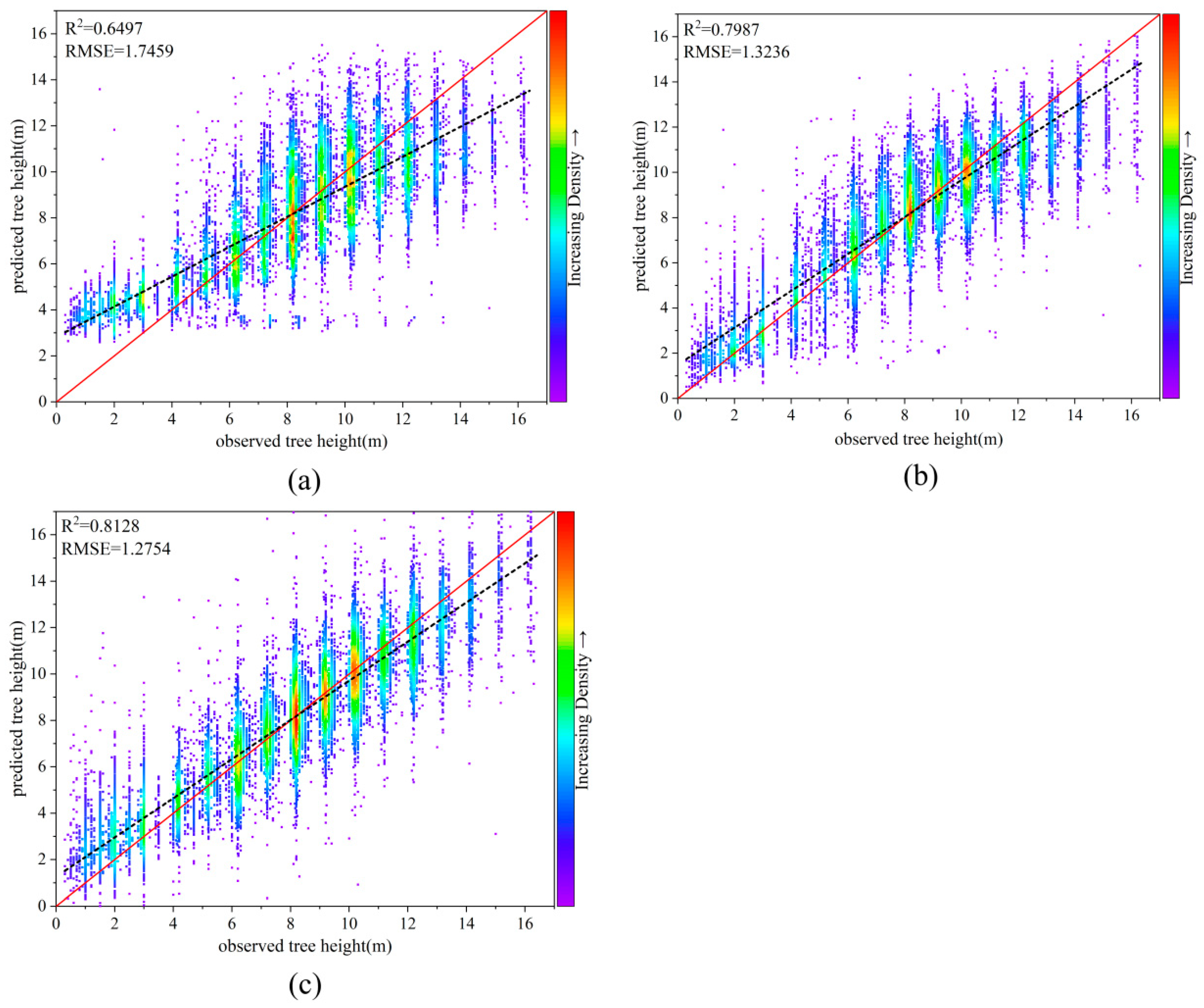
3.2. Comparison of Model Results

The accuracy assessment results for all models based on the test dataset are presented in

Table 3. The model results comparison of the OLS, RF, and GWR.

Model	MAE	RMSE	R2	${\mathbf{R}}_{\mathbf{a}}^2$
OLS	1.3785	1.7459	0.6497	0.6496
RF	0.9524	1.3236	0.7987	0.7986
GWR	0.9305	1.2754	0.8129	0.8128

. Observations indicate that the OLS regression model had the lowest accuracy, with R² and adjusted R² values of only 0.65. Additionally, the OLS model had the highest MAE and RMSE values among the three models, indicating larger prediction errors, averaging 1.3785 m per plot. The RF algorithm achieved a moderate level of accuracy, with R² and adjusted R² slightly below 0.8. Compared to the OLS regression model, there was a significant reduction in both MAE and RMSE. The GWR model performed the best among these three, with R² and adjusted R² above 0.8, and the lowest errors for MAE and RMSE. This indicated that the local-based GWR model had a high level of accuracy and retained an advantage over global models like RF.

Figure 3 describes scatterplots of observed versus estimated values for three models from the test dataset. Consistent conclusions with Table 3 can be drawn from Figure 3: the GWR model demonstrated the highest degree of consistency between predicted and measured tree heights, being closest to the 1:1 line in the figure, and its fitted line (the black dashed line) having the smallest angle with the 1:1 line. The RF model also exhibited moderate accuracy, with its fitted line closely aligning with the 1:1 line. However, the GWR model’s scatter plot distribution conformed more closely to the 1:1 line. Conversely, the OLS model exhibited the poorest predictive accuracy, characterized by the largest angle with the 1:1 line and the most divergent scatter plot distribution. In the lower value range of TH, there was a significant overestimation in the OLS model. In the higher range, there was a significant underestimation. The RF model partially mitigated the overestimation in the lower range of TH; however, underestimation remained evident in the higher range.

3.3. Parameter Estimates with the GWR

After establishing the GWR model, parameter estimates for each feature can be obtained, varying due to differences in geographic location. Therefore, the tree height estimation model established by the GWR model could be considered a model that adjusts according to geographic location. We first performed a statistical analysis of the parameters for each feature to understand their primary distribution (

Table 4. The summary statistics for parameter estimates.

Parameter Estimates	Mean	STD	Median
Intercept	−0.1243	29.0739	0.05119
parameter of elevation	−0.1830	31.1533	−0.0117
parameter of slope	−0.0268	2.2402	−0.0033
parameter of SLT	0.0406	1.3076	0.0278
parameter of UH	0.0098	5.6540	0.0168
parameter of average age	0.8707	0.3085	0.8626

).

Average age showed a clear positive correlation with tree height, while other features exhibited only weak correlations. It should be noted that these statistical results considered all spatial points collectively. However, in some local areas, the correlation between features might be significantly positive or negative.

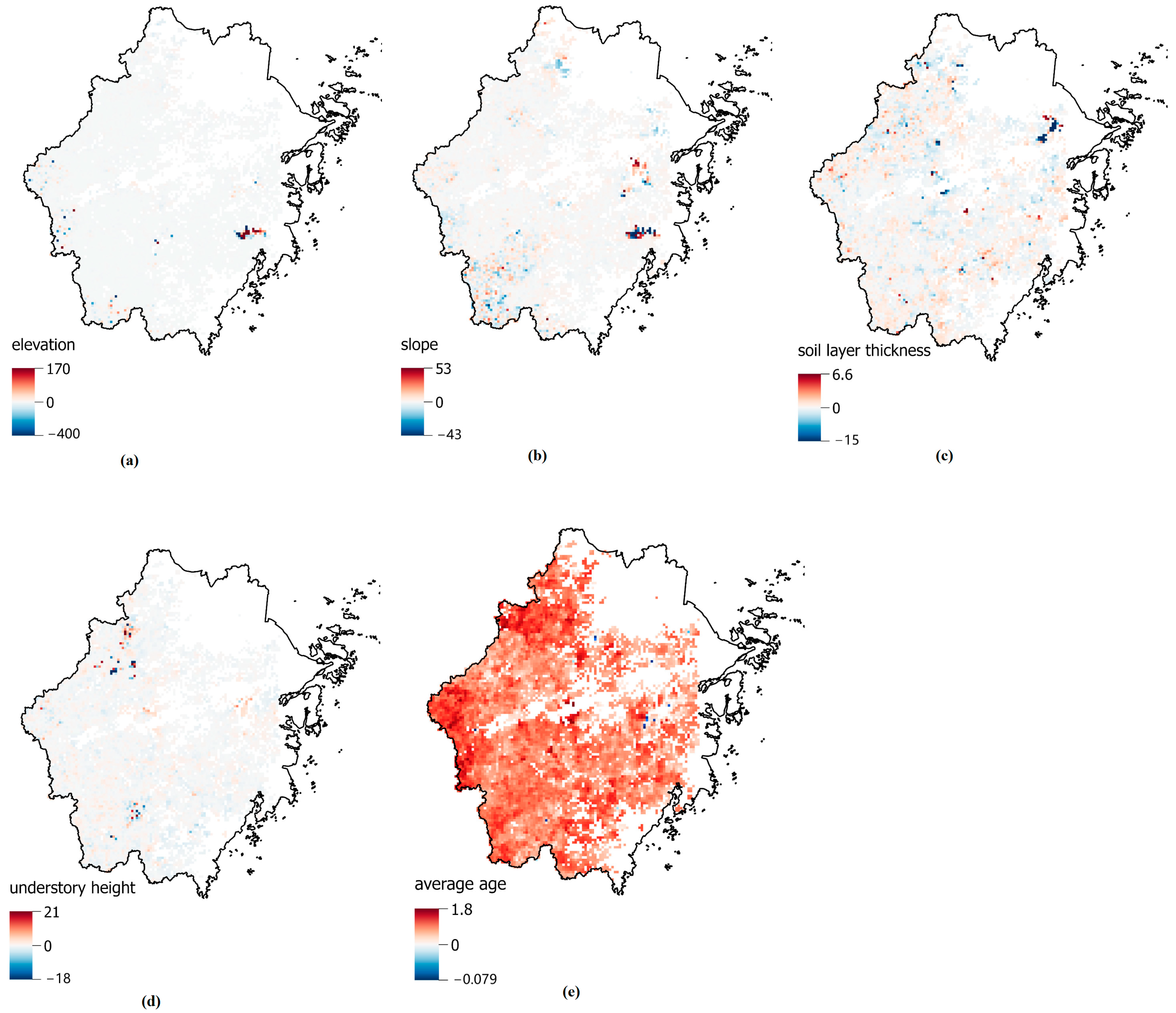
3.4. Spatial Variation of Parameter Estimates

This study visualized and analyzed the spatial variation of parameter estimates at each location within the GWR model. Given the large number of sample points, the study area was initially divided into a grid system to ensure effective visualization. Subsequently, the parameters for the sample points within each grid were averaged. For the analysis conducted at the provincial scale of Zhejiang (Figure 4), a grid size of 3 kilometers was utilized. For displaying the spatial variation of parameter estimates at a smaller scale in detail (Figure 5), a grid size of 1 kilometer was employed.

(a) The parameter related to elevation revealed no distinct correlation with tree height across the province, except for some locations in the Yandang Mountain range. The GWR model’s parameter estimates highlighted spatial heterogeneity in this region.

(b) The parameter for slope paralleled those for elevation, revealing no significant correlation between slope and tree height across most of the province. However, the distribution map captured more detailed information. Observations revealed that the southwestern part of Zhejiang Province exhibited a spatially alternating pattern of positive and negative correlations, whereas the Yandang Mountain range demonstrated a negative correlation, and the Tiantai Mountain in central Zhejiang showed a positive correlation. This suggested that the effects on tree height in mountainous and complex terrain regions exhibited spatial non-stationarity.

(c) The parameter for SLT showed a low correlation with TH. Meanwhile, the spatial non-stationarity was reflected in their relationship in the distribution map, with weak negative and weak positive correlations scattered in different areas. Notably, a substantial negative parameter estimate was identified in the mountainous region to the west of Ningbo City.

(d) The parameter of UH generally indicated a low correlation. However, an elevated positive correlation was observed in the mountainous region of Yuqian town, west of Hangzhou. In contrast, a significant negative correlation was identified in the mountainous areas surrounding Tonglu City and the Thousand Islands Lake region.

(e) The parameter of average age demonstrated a significant positive correlation with tree height across the province. In terms of spatial distribution, a negative correlation was observed in a limited number of mountainous sample points. The spatial distribution map revealed more detailed information, with the magnitude of parameter estimates varying non-uniformly across different spatial locations. Some areas, particularly those around urban centers, had lower parameter estimates, while in the western mountainous region of Hangzhou, Quzhou City in western Zhejiang, and Lishui City had significantly higher parameter estimates. This study focused on the aforementioned areas for a more detailed representation (Figure 5).

4. Discussion

4.1. Tree Height Modeling and Estimation

Forest tree height is an important indicator reflecting the growth and health of forests, and it is also a crucial parameter for estimating forest biomass and carbon storage. It serves as a vital reference for forest management decisions from the national to the regional level. Numerous studies have focused on the estimation of forest tree height, with the majority combining multi-source remote sensing data with ground-survey data [18,20,24]. However, due to the complexity of the study area and the difficulty of data acquisition, large-scale forest tree height estimation studies struggle to achieve fine-scale mapping. Meanwhile, fine-scale local estimation models are challenging to generalize to medium and large regional scales, such as provincial scales. In this study, we utilized nearly 200,000 FMI records to model the tree height of Chinese fir forests, developing a refined estimation model covering Zhejiang Province. We conducted detailed mapping of parameter estimates for each feature and analyzed the spatial variability of their correlations. These research outcomes can enhance our understanding of forest growth conditions and their influencing factors.

This study established a refined tree height estimation model at the provincial scale, facilitated primarily by an extensive collection of ground-survey data. Many studies have utilized data from continuous forest inventories and have achieved good results [29,38]. Owing to variations in sampling methodologies, the FMI data offers comprehensive census data, which have also showcased significant application value in this study.

The height of China’s forests was mapped with R² = 0.6 when evaluated by over 59,000 field plot measurements [24]. The R² and RMSE of another vegetation height product were 0.89 and 4.73 meters, validated by ~400 field measurements [23]. Although our study was on a smaller scale and used different data, the GWR model produced more accurate estimates.

Subsequently, this study conducted a comparison of various estimation models, including the global-based OLS and RF, as well as the local-based GWR model. Our analysis indicated that the GWR model could uncover a more nuanced set of spatial heterogeneity characteristics and portray the spatial variability of different features with greater precision (Figure 5).

Due to data acquisition limitations, only one tree species was considered in this study, and more tree species could be considered to establish models for more systematic research in subsequent studies.

4.2. Global-Based Models and Local-Based Models

OLS and RF are global-based models, meaning that all data collectively contribute to establishing a single model for estimation. During the tree height estimation phase, every data point in space uses the same model parameters for prediction. The spatial characteristics and spatial heterogeneity have been neglected in the model development and estimation phases.

Spatial non-stationarity, which refers to the heterogeneity of spatial characteristics and processes, indicates that the data generation mechanisms differ across various spatial locations. This is manifested by the form or parameters of the corresponding models changing with spatial position [39]. Spatial non-stationarity and heterogeneity are common phenomena in environmental and social science modeling. Forest characteristics and their influencing factors inherently possess spatial heterogeneity, and there is also heterogeneity in the spatial processes among them. This spatial non-stationarity objectively exists, and it should be taken into consideration when modeling. It can be concluded from previous studies that models trained at one study site had higher uncertainty when applied to other sites [19].

Allowing the parameters in spatial models to vary with spatial location can reveal the potentially heterogeneous spatial processes behind the data [25,40]. GWR is one method to achieve this. The spatial variation in GWR parameter estimates, which reflects the relationships between variables, indicates spatial process heterogeneity. For example, although forest average age is directly related to tree height, its parameter estimates may change with different spaces. In this study, we observed spatial heterogeneity in the tree age parameter; in some areas, the correlation between age and tree height was stronger, while in others, it was weaker. Therefore, this non-stationarity of influencing factors in space indicates that global models are not effectively applicable to different spatial locations.

4.3. The Local-Based Geographically Weighted Regression

The GWR estimates regression coefficients for each spatial unit separately using a weighted least squares method, where the weights for each sample decrease with increasing distance [25]. This method can detect differences in the scale of each independent variable’s impact on the dependent variable. It has become one of the most widely used methods for detecting spatial non-stationarity [41]. In GWR, local linear models are calibrated using spatial surrounding data. The result is a series of spatially continuous surfaces showing the location-specific parameter estimates for each independent variable [37]. Additionally, each spatial location has different model parameters. As a result, the tree height estimation model established by the GWR can be considered a series of models that adjust with geographic location. The variation in parameter estimates for each feature reflects the differences in geographic location (Figure 4).

GWR offers two types of spatial kernels: a fixed kernel and an adaptive kernel. A fixed kernel, by definition, uses a consistent bandwidth to delineate a region surrounding each point. The extent of the kernel is uniformly determined by the distance to each spatial point, keeping the size consistent across the space. An adaptive kernel employs a variable bandwidth to define the region surrounding each point. The kernel’s extent is dictated by the number of nearest neighbors around each regression point. Larger bandwidths are applied where data are sparse. Using a fixed kernel means that local regressions for smaller spatial units may incorporate a wider variety of areas. In contrast, local regressions for larger areas might be based on fewer data points, which could lead to estimates with higher standard errors [42]. In our case, the spatial distribution of forest plots in Zhejiang Province is uneven. In the western and southwestern regions of Zhejiang, where the forest coverage is relatively high, the distribution of plots is also denser. In contrast, in the eastern coastal and plain areas of Zhejiang, where the forest coverage is lower, the distribution of plots is sparser. Under these circumstances, this study should use an adaptive kernel to establish the model. These characteristics make the GWR model particularly effective for modeling spatial heterogeneity. In this study, GWR has also demonstrated the effectiveness of the tree-height prediction model.

Nonetheless, the GWR model also possesses certain limitations. With ground-survey data, the collinearity and local collinearity are challenging to mitigate, potentially introducing uncertainty during model development. Investigating methods to enhance the GWR model for multimodal data modeling represents a promising avenue for future research. Concurrently, our findings indicate that GWR, akin to other linear models, is prone to overfitting, for example, when the model exhibits higher training accuracy than testing accuracy. This rationale underpins using a test set in this study to assess and compare the accuracy across different models. Integrating the GWR model with nonlinear models is an emerging research direction. For instance, research has explored integrating GWR with neural networks [26]. In addition, the GWR lacks transfer learning ability. In other words, it is theoretically unreasonable to establish a GWR model by only one region and test it on another region. Instead of building a unified global model, the GWR models establish different models in different spaces. This is the most essential feature of GWR. However, for the global model, transfer learning is easy to achieve if the model accuracy is not taken into account. How to make the local model have better transfer ability is a topic worth studying in the future.

4.4. Spatial Heterogeneity of Feature Impact Effects

In forestry, spatial heterogeneity represents spatial complexity, ecosystem characteristics variability, and heterogeneity in forest vegetation distribution [43]. Recognizing spatial heterogeneity can help us understand the growth changes in forest vegetation and the evolutionary processes of forest ecosystems more effectively [28].

In this study, we visualized and analyzed the spatial variation of the parameter estimates for five characteristics. The spatial distribution maps revealed more detailed information, indicating that the impact of elevation, slope, SLT, UH, and average age on tree height exhibit spatial non-stationarity. For instance, Figure 4d shows the relationship between UH and the height of dominant tree species, demonstrating a positive correlation in some areas and a negative one in others. Forest vegetation growth is influenced by various factors, such as competition from other species and forest disturbances. These interactions among tree species create spatial effects [44,45].

This study primarily revealed the spatial effects of the parameter estimates between age and tree height. We found that the strength of the parameter between the two varies significantly across space. In some areas, such as those around urban regions, the parameter was lower, while in the western mountainous region of Hangzhou, Quzhou City in western Zhejiang, and the Lishui City area, the parameter was noticeably higher. These results reflected the heterogeneity of spatial processes in forests.

5. Conclusions

This study utilized nearly 200,000 ground-survey data points from Zhejiang Province to predict the average tree height of Chinese fir forests. The local-based GWR model was compared with two global-based models, the OLS and RF algorithm. The results showed that the GWR model achieved higher predictive accuracy than OLS and the RF algorithm, with R² and adjusted R² of 0.81 and MAE and RMSE of 0.93 and 1.28, respectively. This suggests that the local GWR model holds advantages over global models, particularly for uncovering spatial non-stationarity in forests.

Through visualization analysis of the parameter estimates across different independent variables, the impact effects of elevation, slope, soil layer thickness, understory height, and average age on tree height exhibit spatial non-stationarity. The spatial distribution maps revealed more detailed information. In mountainous areas with high forest coverage, parameters for average age were notably higher, whereas the parameters were comparatively lower in forests proximate to urban areas.

This study demonstrates the effectiveness of large forest survey datasets and GWR in tree height estimation modeling at a provincial scale. Future research could focus on how to improve the GWR model for its application to multimodal data, as well as how to integrate a variety of algorithms into GWR.

References

1. Lausch, A.; Erasmi, S.; King, D.; Magdon, P.; Heurich, M. Understanding Forest Health with Remote Sensing-Part II—A Review of Approaches and Data Models. Remote Sens. 2017, 9, 129. [Google Scholar] [CrossRef]
2. Guimarães, N.; Pádua, L.; Marques, P.; Silva, N.; Peres, E.; Sousa, J.J. Forestry Remote Sensing from Unmanned Aerial Vehicles: A Review Focusing on the Data, Processing and Potentialities. Remote Sens. 2020, 12, 1046. [Google Scholar] [CrossRef]
3. Asner, G.P. Tropical Forest Carbon Assessment: Integrating Satellite and Airborne Mapping Approaches. Environ. Res. Lett. 2009, 4, 034009. [Google Scholar] [CrossRef]
4. Wang, R.; Gamon, J.A. Remote Sensing of Terrestrial Plant Biodiversity. Remote Sens. Environ. 2019, 231, 111218. [Google Scholar] [CrossRef]
5. Turner, W.; Spector, S.; Gardiner, N.; Fladeland, M.; Sterling, E.; Steininger, M. Remote Sensing for Biodiversity Science and Conservation. Trends Ecol. Evol. 2003, 18, 306–314. [Google Scholar] [CrossRef]
6. Torresani, M.; Rocchini, D.; Sonnenschein, R.; Zebisch, M.; Hauffe, H.C.; Heym, M.; Pretzsch, H.; Tonon, G. Height Variation Hypothesis: A New Approach for Estimating Forest Species Diversity with CHM LiDAR Data. Ecol. Indic. 2020, 117, 106520. [Google Scholar] [CrossRef]
7. Yu, Z.; Liu, S.; Li, H.; Liang, J.; Liu, W.; Piao, S.; Tian, H.; Zhou, G.; Lu, C.; You, W.; et al. Maximizing Carbon Sequestration Potential in Chinese Forests through Optimal Management. Nat. Commun. 2024, 15, 3154. [Google Scholar] [CrossRef] [PubMed]
8. Huang, Y.; Sun, W.; Qin, Z.; Zhang, W.; Yu, Y.; Li, T.; Zhang, Q.; Wang, G.; Yu, L.; Wang, Y.; et al. The Role of China’s Terrestrial Carbon Sequestration 2010–2060 in Offsetting Energy-Related CO2 Emissions. Natl. Sci. Rev. 2022, 9, nwac057. [Google Scholar] [CrossRef]
9. Tang, X.; Zhao, X.; Bai, Y.; Tang, Z.; Wang, W.; Zhao, Y.; Wan, H.; Xie, Z.; Shi, X.; Wu, B.; et al. Carbon Pools in China’s Terrestrial Ecosystems: New Estimates Based on an Intensive Field Survey. Proc. Natl. Acad. Sci. USA 2018, 115, 4021–4026. [Google Scholar] [CrossRef]
10. Shang, R.; Chen, J.M.; Xu, M.; Lin, X.; Li, P.; Yu, G.; He, N.; Xu, L.; Gong, P.; Liu, L.; et al. China’s Current Forest Age Structure Will Lead to Weakened Carbon Sinks in the near Future. Innovation 2023, 4, 100515. [Google Scholar] [CrossRef]
11. Xie, X.; Wang, Q.; Dai, L.; Su, D.; Wang, X.; Qi, G.; Ye, Y. Application of China’s National Forest Continuous Inventory Database. Environ. Manag. 2011, 48, 1095–1106. [Google Scholar] [CrossRef] [PubMed]
12. Zeng, W.; Tomppo, E.; Healey, S.P.; Gadow, K.V. The National Forest Inventory in China: History-Results-International Context. For. Ecosyst. 2015, 2, 23. [Google Scholar] [CrossRef]
13. Fang, N.; Yao, L.; Wu, D.; Zheng, X.; Luo, S. Assessment of Forest Ecological Function Levels Based on Multi-Source Data and Machine Learning. Forests 2023, 14, 1630. [Google Scholar] [CrossRef]
14. Fang, G.; Xu, H.; Yang, S.-I.; Lou, X.; Fang, L. Synergistic Use of Sentinel-1, Sentinel-2, and Landsat 8 in Predicting Forest Variables. Ecol. Indic. 2023, 151, 110296. [Google Scholar] [CrossRef]
15. Huang, H.; Wu, D.; Fang, L.; Zheng, X. Comparison of Multiple Machine Learning Models for Estimating the Forest Growing Stock in Large-Scale Forests Using Multi-Source Data. Forests 2022, 13, 1471. [Google Scholar] [CrossRef]
16. McCombs, J.W.; Roberts, S.D.; Evans, D.L. Influence of Fusing Lidar and Multispectral Imagery on Remotely Sensed Estimates of Stand Density and Mean Tree Height in a Managed Loblolly Pine Plantation. For. Sci. 2003, 49, 457–466. [Google Scholar] [CrossRef]
17. Wilkes, P.; Jones, S.; Suarez, L.; Mellor, A.; Woodgate, W.; Soto-Berelov, M.; Haywood, A.; Skidmore, A. Mapping Forest Canopy Height Across Large Areas by Upscaling ALS Estimates with Freely Available Satellite Data. Remote Sens. 2015, 7, 12563–12587. [Google Scholar] [CrossRef]
18. Su, Y.; Ma, Q.; Guo, Q. Fine-Resolution Forest Tree Height Estimation across the Sierra Nevada through the Integration of Spaceborne LiDAR, Airborne LiDAR, and Optical Imagery. Int. J. Digit. Earth 2017, 10, 307–323. [Google Scholar] [CrossRef]
19. García, M.; Saatchi, S.; Ustin, S.; Balzter, H. Modelling Forest Canopy Height by Integrating Airborne LiDAR Samples with Satellite Radar and Multispectral Imagery. Int. J. Appl. Earth Obs. Geoinf. 2018, 66, 159–173. [Google Scholar] [CrossRef]
20. Lin, X.; Shang, R.; Chen, J.M.; Zhao, G.; Zhang, X.; Huang, Y.; Yu, G.; He, N.; Xu, L.; Jiao, W. High-Resolution Forest Age Mapping Based on Forest Height Maps Derived from GEDI and ICESat-2 Space-Borne Lidar Data. Agric. For. Meteorol. 2023, 339, 109592. [Google Scholar] [CrossRef]
21. Lefsky, M.A. A Global Forest Canopy Height Map from the Moderate Resolution Imaging Spectroradiometer and the Geoscience Laser Altimeter System. Geophys. Res. Lett. 2010, 37, 2010GL043622. [Google Scholar] [CrossRef]
22. Costa, E.A.; Hess, A.F.; Finger, C.A.G.; Schons, C.T.; Klein, D.R.; Barbosa, L.O.; Borsoi, G.A.; Liesenberg, V.; Bispo, P.D.C. Enhancing Height Predictions of Brazilian Pine for Mixed, Uneven-Aged Forests Using Artificial Neural Networks. Forests 2022, 13, 1284. [Google Scholar] [CrossRef]
23. Huang, H.; Liu, C.; Wang, X.; Biging, G.S.; Chen, Y.; Yang, J.; Gong, P. Mapping Vegetation Heights in China Using Slope Correction ICESat Data, SRTM, MODIS-Derived and Climate Data. ISPRS J. Photogramm. Remote Sens. 2017, 129, 189–199. [Google Scholar] [CrossRef]
24. Liu, X.; Su, Y.; Hu, T.; Yang, Q.; Liu, B.; Deng, Y.; Tang, H.; Tang, Z.; Fang, J.; Guo, Q. Neural Network Guided Interpolation for Mapping Canopy Height of China’s Forests by Integrating GEDI and ICESat-2 Data. Remote Sens. Environ. 2022, 269, 112844. [Google Scholar] [CrossRef]
25. Brunsdon, C.; Fotheringham, A.S.; Charlton, M.E. Geographically Weighted Regression: A Method for Exploring Spatial Nonstationarity. Geogr. Anal. 1996, 28, 281–298. [Google Scholar] [CrossRef]
26. Du, Z.; Wang, Z.; Wu, S.; Zhang, F.; Liu, R. Geographically Neural Network Weighted Regression for the Accurate Estimation of Spatial Non-Stationarity. Int. J. Geogr. Inf. Sci. 2020, 34, 1353–1377. [Google Scholar] [CrossRef]
27. Tu, J. Spatially Varying Relationships between Land Use and Water Quality across an Urbanization Gradient Explored by Geographically Weighted Regression. Appl. Geogr. 2011, 31, 376–392. [Google Scholar] [CrossRef]
28. Wang, Q.; Ni, J.; Tenhunen, J. Application of a Geographically-weighted Regression Analysis to Estimate Net Primary Production of Chinese Forest Ecosystems. Glob. Ecol. Biogeogr. 2005, 14, 379–393. [Google Scholar] [CrossRef]
29. Liu, H.; Fu, Y.; Pan, J.; Wang, G.; Hu, K. Biomass Spatial Pattern and Driving Factors of Different Vegetation Types of Public Welfare Forests in Hunan Province. Forests 2023, 14, 1061. [Google Scholar] [CrossRef]
30. Chen, L.; Ren, C.; Zhang, B.; Wang, Z.; Xi, Y. Estimation of Forest Above-Ground Biomass by Geographically Weighted Regression and Machine Learning with Sentinel Imagery. Forests 2018, 9, 582. [Google Scholar] [CrossRef]
31. Zhang, X.; Sun, Y.; Jia, W.; Wang, F.; Guo, H.; Ao, Z. Research on the Temporal and Spatial Distributions of Standing Wood Carbon Storage Based on Remote Sensing Images and Local Models. Forests 2022, 13, 346. [Google Scholar] [CrossRef]
32. Chen, F.-S.; Niklas, K.J.; Liu, Y.; Fang, X.-M.; Wan, S.-Z.; Wang, H. Nitrogen and Phosphorus Additions Alter Nutrient Dynamics but Not Resorption Efficiencies of Chinese Fir Leaves and Twigs Differing in Age. Tree Physiol. 2015, 35, 1106–1117. [Google Scholar] [CrossRef] [PubMed]
33. Zhejiang Provincial Forestry Department. Technical Regulations of Forest Resources Planning and Design Survey in Zhejiang Province (in Chinese); Zhejiang Provincial Forestry Department: Hangzhou, China, 2014. [Google Scholar]
34. Breiman, L. Random Forests. Mach. Learn. 2001, 45, 5–32. [Google Scholar] [CrossRef]
35. George, C.S.; Sumathi, B. Grid Search Tuning of Hyperparameters in Random Forest Classifier for Customer Feedback Sentiment Prediction. IJACSA 2020, 11. [Google Scholar] [CrossRef]
36. Rey, S.J.; Anselin, L. PySAL: A Python Library of Spatial Analytical Methods. In Handbook of Applied Spatial Analysis; Fischer, M.M., Getis, A., Eds.; Springer Berlin Heidelberg: Berlin/Heidelberg, Germany, 2010; pp. 175–193. ISBN 978-3-642-03646-0. [Google Scholar]
37. Oshan, T.; Li, Z.; Kang, W.; Wolf, L.; Fotheringham, A. Mgwr: A Python Implementation of Multiscale Geographically Weighted Regression for Investigating Process Spatial Heterogeneity and Scale. IJGI 2019, 8, 269. [Google Scholar] [CrossRef]
38. Wu, S.; Sun, Y.; Jia, W.; Wang, F.; Lu, S.; Zhao, H. Estimation of Above-Ground Carbon Storage and Light Saturation Value in Northeastern China’s Natural Forests Using Different Spatial Regression Models. Forests 2023, 14, 1970. [Google Scholar] [CrossRef]
39. Liu, Y.; Wang, K.; Xing, X.; Guo, H.; Zhang, W. On Spatial Effects in Geographical Analysis. Acta Geogr. Sin. 2023, 78, 517–531. [Google Scholar]
40. Fotheringham, A.S.; Brunsdon, C. Local Forms of Spatial Analysis. Geogr. Anal. 1999, 31, 340–358. [Google Scholar] [CrossRef]
41. Fotheringham, A.S.; Yang, W.; Kang, W. Multiscale Geographically Weighted Regression (MGWR). Ann. Am. Assoc. Geogr. 2017, 107, 1247–1265. [Google Scholar] [CrossRef]
42. Suryowati, K.; Ranggo, M.O.; Bekti, R.D.; Sutanta, E.; Riswanto, E. Geographically Weighted Regression Using Fixed and Adaptive Gaussian Kernel Weighting for Maternal Mortality Rate Analysis. In Proceedings of the 2021 3rd International Conference on Electronics Representation and Algorithm (ICERA), Yogyakarta, Indonesia, 29 July 2021; pp. 115–120. [Google Scholar]
43. Haining, R.; Zhang, J. Spatial Data Analysis: Theory and Practice; Cambridge University Press: Cambridge, UK, 2003. [Google Scholar]
44. Junttila, V.; Laine, M. Bayesian Principal Component Regression Model with Spatial Effects for Forest Inventory Variables under Small Field Sample Size. Remote Sens. Environ. 2017, 192, 45–57. [Google Scholar] [CrossRef]
45. Han, N.; Du, H.; Zhou, G.; Xu, X.; Cui, R.; Gu, C. Spatiotemporal Heterogeneity of Moso Bamboo Aboveground Carbon Storage with Landsat Thematic Mapper Images: A Case Study from Anji County, China. Int. J. Remote Sens. 2013, 34, 4917–4932. [Google Scholar] [CrossRef]
Figure 1. The location of the study area and the spatial distribution of FMI plots. (a) The study area is located in Zhejiang Province, China. (b) The FMI plots of the Chinese fir forest in Zhejiang Province, to clearly represent the spatial distribution of survey points and for the convenience of subsequent data processing, the vector data of the sub-compartments in this study were converted into centroid point data of the plots. (b) shows that the samples basically cover all forest areas in Zhejiang Province, excluding the islands. The FMI plots exhibit a fairly high spatial density, especially in areas with dense forest cover. (c) Sample of FMI plots after zooming in.
Forests 15 01315 g001
Figure 2. The flowchart of this study.
Forests 15 01315 g002
Figure 3. Scatterplots based on density color of observed versus predicted TH for three models, The OLS, RF, and GWR models are depicted in (a), (b), and (c), respectively. The red line in the figures represents the 1:1 line, and the black dashed line represents the fitted line between the predicted and observed TH.
Forests 15 01315 g003
Figure 4. The spatial distribution of parameter estimates for (a) elevation, (b) slope, (c) soil layer thickness, (d) understory height, and (e) average age. To compare the variation in these parameter estimates consistently, red in the figure represents positive parameter estimates, and blue represents negative parameter estimates, and the deeper the color, the higher the parameter estimates. White represents parameter estimates close to zero, indicating a weak correlation.
Forests 15 01315 g004
Figure 5. Local magnification of the parameter estimates for average age: (a) the western mountainous region of Hangzhou, (b) the western Zhejiang (Quzhou city), and (c) the southwestern Zhejiang (Lishui City).
Forests 15 01315 g005