Article

Projecting the Impacts of Climate Change, Soil, and Landscape on the Geographic Distribution of Ma Bamboo (Dendrocalamus latiflorus Munro) in China

1
College of Landscape Architecture and Art, Fujian Agriculture and Forestry University, Fuzhou 350002, China
2
College of Forestry, Fujian Agriculture and Forestry University, Fuzhou 350002, China
*
Author to whom correspondence should be addressed.
Forests 2024, 15(8), 1321; https://doi.org/10.3390/f15081321 (registering DOI)
Submission received: 5 July 2024 / Revised: 25 July 2024 / Accepted: 25 July 2024 / Published: 29 July 2024
(This article belongs to the Section Forest Ecology and Management)

Abstract

:
Ma bamboo (Dendrocalamus latiflorus Munro) is a fast-growing woody grass that offers significant economic benefits, including materials for construction, furniture, biofuel, food, and handicrafts. It also provides ecological benefits like soil conservation, wildlife habitats, and carbon sequestration. However, its species distribution patterns are influenced by various factors, including climate (mainly temperature and precipitation), soil attributes, and landscape characteristics such as topography, land use, and vegetation. Understanding these impacts is essential for the sustainable management of D. latiflorus resources and fostering related economic activities. To address these challenges, we developed a comprehensive habitat suitability (CHS) model that integrates climate, soil, and landscape variables to simulate the distribution dynamics of D. latiflorus under different shared socio-economic pathway (SSP) scenarios. An ensemble model (EM) strategy was applied to each variable set to ensure robust predictions. The results show that the current potential distribution of D. latiflorus spans 28.95 × 10⁴ km2, primarily located in South China and the Sichuan Basin. Its distribution is most influenced by the annual mean temperature (Bio1), the cation exchange capacity of soil clay particles in the 20–40 cm soil layer (CECc 20–40 cm), vegetation, and elevation. Under future climate scenarios, these habitats are projected to initially expand slightly and then contract, with a northward shift in latitude and migration to higher elevations. Additionally, the Sichuan Basin (Sichuan–Chongqing border) is identified as a climatically stable area suitable for germplasm development and conservation. To conclude, our findings shed light on how climate change impacts the geographic distribution of D. latiflorus, providing key theoretical foundations for its sustainable cultivation and conservation strategies.

1. Introduction

In the face of climate change’s escalating effects, the demand for sustainable materials has become paramount. Bamboo, with its unique characteristics such as rapid growth, swift forest formation, prolonged usability, brief production cycles, high yield, and strong carbon absorption capacity, represents a viable alternative to environmentally detrimental and resource-intensive materials, offering a glimmer of hope amidst this global crisis [1]. Moreover, bamboo forests offer considerable carbon sink potential [2]. For example, Moso bamboo (Phyllostachys edulis (Carrière) J. Houzeau) forests can capture 4.91–5.45 t C ha 1 yr 1 , which is 1.41–1.57 times greater than the capture rate of fast-growing Chinese fir (Cunninghamia lanceolata (Lamb.) Hook.) plantations [3]. In China, the bamboo industry creates 8 million jobs and generates USD 28 billion in output annually, aiding poverty reduction, enhancing human livelihoods, promoting sustainable economic growth, and addressing climate change [4]. Despite the diversity of bamboo species, only a few, including Moso bamboo (P. edulis), Ma bamboo (Dendrocalamus latiflorus Munro), and Lei bamboo (Phyllostachys violascens ‘Prevernalis’ S.Y.Chen et C.Y.Yao) meet the criteria for industrial utilization [5]. Accurate spatial distribution data inform government policies, optimize industrial layout, and ensure efficient resource allocation, thereby supporting sustainable cultivation practices, maximizing productivity, and balancing economic growth with ecological sustainability. Therefore, predicting their potential spatial distribution is crucial for the sustainable management of eco-friendly and economically significant bamboo resources.
Bamboo is highly susceptible to climate change due to its rapid growth rate, which is dependent on high rates of photosynthesis and water uptake, making it sensitive to variations in temperature and precipitation [6,7]. Moreover, bamboo species exhibit unusual sexual reproduction intervals ranging from 10 to 120 years [8], coupled with limited seed dispersal capabilities [9]. The vegetative dispersal ability of bamboo also varies significantly; for instance, many understory species have restricted spread, such as Bashania fargesii (E. G. Camus) Keng f. et Yi, which disperses only about 0.2–0.35 m yr 1 [10]. These constraints collectively hinder bamboo’s capacity to adjust its geographical distribution in response to the rapid climate changes projected for this century. In China, climate change is expected to lead to global warming, more heatwaves, uneven rainfall distribution, and monsoon variability, causing bamboo forests to potentially migrate northward in Southeastern China and southward in Southwestern China for refuge [4,11]. Despite favorable climatic conditions, bamboo growth can be significantly restricted without appropriate soil and landscape conditions, including topography, land use, and vegetation. To address the impact of complex environmental filtering on bamboo resources, species distribution models (SDMs) are frequently employed [12]. These models help predict the potential distribution of bamboo species under varying environmental conditions, providing valuable insights for conservation and sustainable management.
SDMs, also known as ecological niche models (ENMs), are widely employed to predict the potential spatial and temporal distribution of species on a large scale [12,13,14,15]. By linking species occurrence data to environmental variables and employing statistical techniques, SDMs are able to map and predict species distributions across various spatial and temporal dimensions [13,16]. The emergence of new statistical algorithms and software applications has made the description and prediction of distribution patterns more reliable [17,18,19,20]. Popular algorithms include artificial neural networks (ANNs) [21], classification tree analysis (CTA) [22], flexible discriminant analysis (FDA) [23], generalized additive models (GAMs) [24], generalized boosting models (GBMs) [25], generalized linear models (GLMs) [26], multiple adaptive regression splines (MARS) [27], maximum entropy (MaxEnt) [28], MaxEnt over glmnet (MaxNet) [29], random forest (RF) [30], surface range envelope (SRE, i.e., BIOCLIM) [31], and extreme gradient boosting training (XGBOOST) [32]. However, the selection of optimal algorithms for particular species under designated spatio-temporal contexts varies due to niche properties, habitat complexity, and data resolution and precision [14,33]. Therefore, ensemble models (EMs), which combine the relative importance of individual models built with different algorithms, have been proposed to address this issue [34,35]. The EM strategy avoids the model bias that arises from the selection of a single optimal algorithm, thereby providing more robust and accurate predictions [36,37].
Ma bamboo (Dendrocalamus latiflorus Munro) is a fast-growing, evergreen, giant, semitropical clumping bamboo species native to Southeast China, known for its widespread distribution across the region. It holds high biological, ecological, industrial, culinary, and medicinal value [5,6,38,39,40,41,42]. D. latiflorus significantly contributes to carbon sequestration, with its aboveground carbon storage (48.94 ± 41.06 M g ha 1 ) exceeding that of Moso bamboo and Makino bamboo [39]. Its complex rhizome–root system prevents soil erosion and promotes water percolation, outperforming both broad-leaved and coniferous forests [38]. Understorey D. latiflorus forest are an essential component in many forest ecosystems [43], enhancing species composition and structural complexity, and providing vital resources for wildlife [6]. Additionally, bamboo is used in paper making, tool crafting, rafts, handicrafts, and building materials. Bamboo shoots are edible, its leaves are used for wrapping zongzi and making wine, and both the flowers and shoots can treat coughs [44]. Our field investigations reveal that, beyond the influences of temperature and precipitation, as demonstrated by previous studies [4,45], the growth of D. latiflorus is significantly constrained by the absence of suitable soil and landscape conditions, including topography, land use, and vegetation. Specifically, D. latiflorus thrives in regions with a subtropical or temperate climate, characterized by annual average temperatures of 8–26 °C and annual precipitation of 800–3300 mm. It flourishes on gentle slopes up to 1000 m in shrubland and woodland environments, where the soil consists of reddish and brownish loams. The soil moisture content in these habitats typically ranges between 20% and 40%. To address the cumulative environmental impacts on the species, previous studies [14,15,16,46,47] have developed a comprehensive habitat suitability (CHS) model to more precisely evaluate a species’ suitable habitat, incorporating climate variables along with soil, topography, vegetation, and land-cover factors.
Previous studies on D. latiflorus have primarily focused on its sequence, purification and structural identification, cultivation, biomass and carbon storage, and industrialization [48,49,50,51,52,53,54]. Nonetheless, the projected current and future distribution of D. latiflorus, as well as the effects of environmental factors on its range, have rarely been investigated within the framework of climate change. Although previous studies [4,55,56] have examined the potential distribution of Chinese bamboo forests, detailed information on individual bamboo species remains scarce. Accordingly, we applied the CHS model, combining climate, soil, and landscape attributes, to project the potential distribution of D. latiflorus across different climate change scenarios. Species distribution data were obtained from both field surveys and online databases. The aims of this research are threefold: (1) to assess how climatic, soil, and landscape variables influence the geographic distribution of D. latiflorus and to identify the primary constraints on its distribution; (2) to build a CHS model that predicts the potential distribution of D. latiflorus, incorporating the cumulative effects of climate, soil, and landscape conditions; and (3) to quantify and compare the spatial pattern differences under current and future climate change scenarios, specifically across three periods (2021–2040, 2041–2060, and 2061–2080) with four CMIP6 shared socio-economic pathways (SSPs: SSP1-RCP2.6, SSP2-RCP4.5, SSP3-RCP7.0, and SSP5-RCP8.5).

2. Materials and Methods

Figure 1 illustrates the workflow for the habitat suitability assessment. The specific steps are as follows:

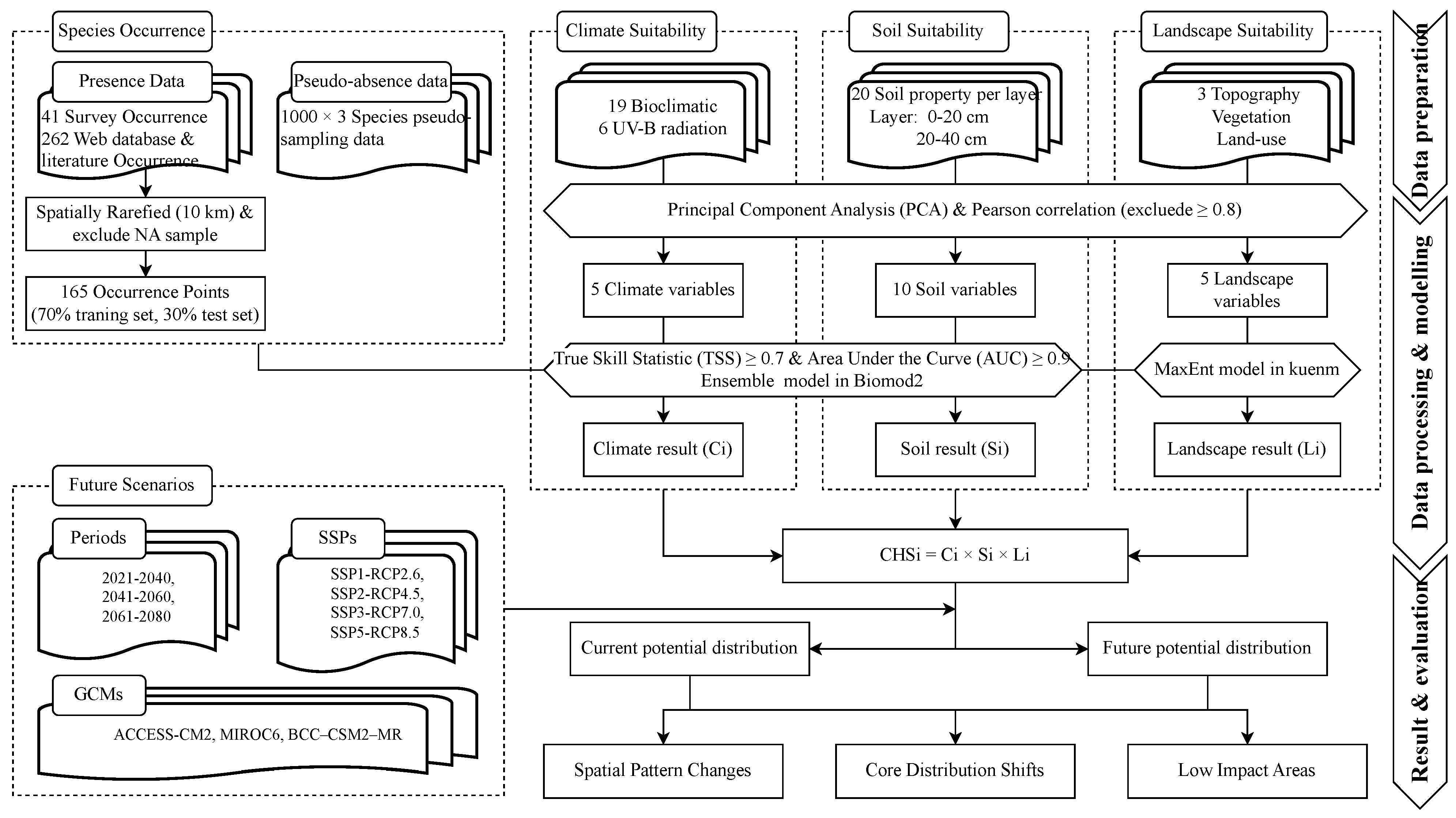
2.1. Data Preparation and Processing

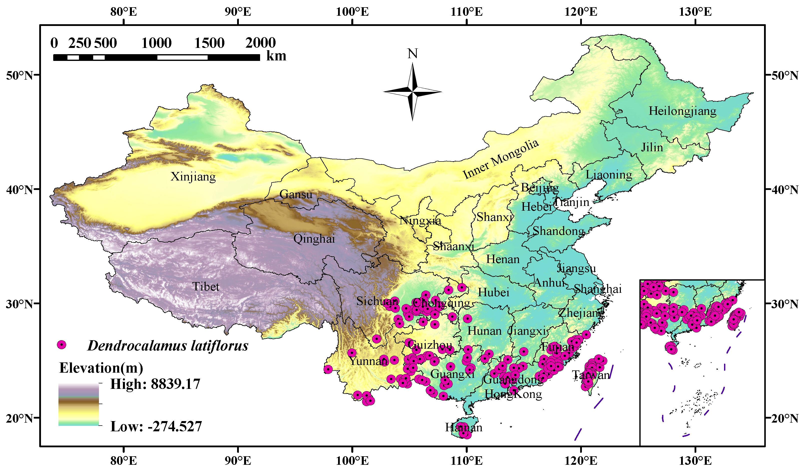
2.1.1. Species Occurrence and Pseudo-Absence Data

Over the last five years, from March 2018 to October 2023, extensive field surveys were conducted in the provinces of Fujian, Jiangxi, Guangdong, Guangxi, Sichuan, Chongqing, Guizhou, and Yunnan. These regions encompass the most recorded distributions according to the Flora of China (http://www.efloras.org, accessed on 3 September 2023). By designating the center of each investigated D. latiflorus forest as a distribution point, we identified 41 occurrence points. Additionally, 262 valid, non-replicate occurrence points were sourced from various web databases and previously published literature, including the Global Biodiversity Information Facility (GBIF, https://www.gbif.org, accessed on 12 March 2024), Chinese National Science and Technology Infrastructure (NSII, http://www.nsii.org.cn, accessed on 12 March 2024), Plant Photo Bank of China (PPBC, https://ppbc.iplant.cn, accessed on 12 March 2024), Chinese Virtual Herbarium (CVH, https://www.cvh.ac.cn, accessed on 12 March 2024), China National Knowledge Infrastructure (CNKI, https://www.cnki.net, accessed on 12 March 2024), and Google Scholar. To minimize spatial auto-correlation, a 10 × 10 km grid cell was used to exclude any occurrence points within 10 km of another point using the Spatially Rarefy Occurrence Data tool in SDMtoolbox v2.6 [57,58]. We also excluded 18 occurrences where environmental variables were missing. As a result, 165 occurrence points were finalized for use in the modeling process (Figure 2; Table S1).
Predictions from SDMs that rely on presence-only data are significantly influenced by the quality and quantity of pseudo-absence data [16,59]. To enhance the accuracy of SDMs, this study generated three sets of 1000 pseudo-absence points each by randomly sampling the background area [14,16].

2.1.2. Climatic, Soil, and Landscape Variables

The relevance and completeness of predictors are critical components in constructing SDMs [14,60,61]. Numerous biotic and abiotic factors, including climate, topography, soil, vegetation, land use, and other environmental parameters, influence plant lifecycle processes, thereby shaping their distribution. Therefore, we categorized the environmental datasets into three types: climate, soil, and landscape variables, encompassing a total of 72 environmental variables (Table S2).
The climate variables included 19 bioclimatic layers obtained from the WorldClim dataset (https://www.worldclim.org, accessed on 4 April 2024) for both current and future periods, with a spatial resolution of 30″ (approximately 1 km2) [62]. The current climate data represent the average conditions from 1970 to 2000. Future climate data for the 2030s (2021–2040), 2050s (2041–2060), and 2070s (2061–2080) were obtained from four SSPs (SSP1-RCP2.6, SSP2-RCP4.5, SSP3-RCP7.0, and SSP5-RCP8.5) and averaged from three global climate models (GCMs) commonly used in China and Asia: ACCESS-CM2, MIROC6, and BCC-CSM2-MR [63,64,65]. Additionally, the Global UV-B radiation dataset was obtained from the gIUV database (https://www.ufz.de/gluv/, accessed on 4 April 2024) [66].
The soil data were obtained from the China soil property raster dataset available at the National Cryosphere Desert Data Center (https://www.ncdc.ac.cn, accessed on 4 April 2024) [67]. This dataset is derived from the global-scale soil properties database WISE30sec, produced by the International Soil Reference and Information Centre (ISRIC) [68]. It contains 20 soil properties across seven depth layers (Table S2). Given that 80%–90% of bamboo roots are located within the 0–40 cm depth range [69,70], the data for the 0–20 cm and 20–40 cm layers were selected for this study, resulting in a total of 40 soil variables.
The landscape variables included topography, vegetation, and land use. The topographic variables, such as elevation, slope, and aspect, were sourced from MERIT DEM (http://hydro.iis.u-tokyo.ac.jp/~yamadai/MERIT_DEM/, accessed on 16 January 2024) [71], with slope and aspect generated using the ArcGIS spatial analysis function based on the elevation data. Vegetation data were obtained from the 1:1 million vegetation dataset in China [72], and land-use data were acquired from the 1:1 million comprehensive land cover dataset of China [73]. Both the vegetation and land-use datasets were accessed from the National Cryosphere Desert Data Center (https://www.ncdc.ac.cn, accessed on 4 April 2024).

2.1.3. Data Processing and Variable Screening

The present study resampled all variable layers to a 30″ spatial resolution, clipped to the China boundary range and projected using the WGS_1984_Albers coordinate system. To prevent overfitting and address multicollinearity within the three variable sets, we implemented a two-step procedure [15,74].
First, Principal Component Analysis (PCA) was conducted to identify subsets of climatic, soil, and landscape variables [14,37]. The number of principal components was determined based on cumulative variance, and a subset of variables was chosen according to their contributions to these components. Next, Pearson correlation coefficients were calculated for each pairwise comparison of the filtered variables. Only the most significant variables were retained when strong correlations ( r 0.8 ) were detected, based on their contribution values and ecological significance (Figure S1).
Following these analyses, five climate variables were identified: annual mean temperature (Bio1), mean temperature of warmest quarter (Bio10), annual precipitation (Bio12), precipitation of driest quarter (Bio17), and annual mean UV-B (UVB1). Additionally, ten soil variables were determined (TOTN 20–40 cm, PHAQ 0–20 cm, CECs 20–40 cm, ECEC 0–20 cm, CECc 20–40 cm, TAWC 0–20 cm, STPC 20–40 cm, ALSA 20–40 cm, ELCO 0–20 cm, and CNrt 20–40 cm), along with three topographic variables, one vegetation variable, and one land-use variable. In total, 20 environmental variables were retained to model the distribution of D. latiflorus (Table S2).

2.2. Development of Comprehensive Habitat Suitability Model

Following previous studies [14,15,16], we developed a CHS model to evaluate the potential distribution of D. latiflorus, incorporating climatic, soil, and landscape limitations (Figure 1). Initially, we constructed three individual sub-models: the climatic EM, the soil EM, and the landscape MaxEnt model. These sub-models were then integrated to form the CHS model, which accounts for the cumulative effects of each category. Each sub-model is equally important, and the species is considered suitable for growth only when the cumulative criteria are met.

2.2.1. Ensemble Model for Climate and Soil Suitability

The EM strategy was employed to separately analyze climate and soil suitability. Twelve algorithms were selected for this purpose: ANN, CTA, FDA, GAM, GBM, GLM, MARS, MaxEnt, MaxNet, RF, SRE, and XGBOOST. All model-building processes were conducted using the BIOMOD2 package [20] in R software (version 4.3.2) [75].
First, we filtered algorithms for building the EM. The 165 occurrence points were divided into 70% for model calibration and 30% for model validation. We constructed a total of 360 single models, including three pseudo-absence sampling models, twelve algorithms, and ten cross-validation runs for each of climate and soil suitability. Only algorithms with a mean true skill statistic (TSS) of ≥0.7 and an area under the curve (AUC) of ≥0.9 in both the calibration and validation steps were retained for the ensemble forecast. For the climate EM, nine algorithms (ANN, FDA, GAM, GBM, GLM, MARS, MaxEnt, MaxNet, and XGBOOST) met the criteria and exhibited high evaluation scores. For the soil EM, only GBM met the standard (Figure S2).
Second, we generated the EM. To create the EM, we applied the weighted average method to combine all single models that had TSS values of ≥0.7 and AUC ≥ 0.9. The weights of each single model were determined using the TSS values, as shown in Equation (1):
w j = r j j = 1 h r j
where w j is the weight of model result j; r j is the TSS value of model result j; and h is the number of model results. The normalized results of a single model were then multiplied by the corresponding weight to obtain the summation.
Third, we calculated the suitability index for both climate and soil EMs as described in Equation (2):
y i = j = 1 n w j × x i j
where y i is the potential habitat suitability index of the first grid i; w j is the weight of SDM j; x i j is the value of grid i in SDM j; and y i (range 0 , 1 ) is the evaluation index for the distribution of potentially suitable D. latiflorus habitats.

2.2.2. MaxEnt Model for Landscape Suitability

Among the twelve algorithms, only the MaxEnt model can use categorical data as environmental variable inputs [14]. Therefore, we employed the MaxEnt model with the 165 occurrence data (70% for training and 30% for testing) to determine the landscape constraints of D. latiflorus. The kuenm package [19] was utilized to optimize the feature class (FC) and regularization multiplier (RM) of the MaxEnt model. Initially, the RM was set to range from 0.1 to 10 with intervals of 0.1, resulting in a total of 100 RM values. Subsequently, the five FCs (linear (l), quadratic (q), product (p), threshold (t), and hinge (h)) in the MaxEnt model were combined to form 31 FC combinations (e.g., l, q, p, t, h, lq, lp, lt, lh, qp, qt, qh, pt, ph, th, lqp, lqt, lqh, lpt, lph, lth, qpt, qph, qth, pth, lqpt, lqph, lqth, lpth, qpth, and lqpth). Thus, a total of 3100 parameter combinations were tested by multiplying the FCs and RMs.
For optimal model determination, the model with a significant omission rate (OR) of ≤0.05 and a delta AICc ( Δ AICc ) of ≤2 was selected [76]. The optimal parameters indicated that the FC and RM were pth and 1.8, respectively (Figure S3).

2.2.3. Comprehensive Habitat Suitability Model

Based on the climatic and soil EMs, as well as the landscape MaxEnt model, we constructed a CHS model to evaluate the suitability index of D. latiflorus habitats. The suitability index of the CHS model for each evaluation grid is described by Equation (3):
C H S i = C i × S i × L i
where C H S i is the comprehensive habitat suitability index in each evaluation grid; C i is the occurrence probability of the climatic EM based on 4 bioclimatic variables and one UV-B radiation variable; S i is the occurrence probability of the soil EM based on 10 soil variables; and L i is the occurrence probability of the landscape MaxEnt model based on three topographic, vegetation, and land-use variables. The cumulative occurrence probability of C H S i ranges from 0 to 1.
Following previous studies [14,15,16], C H S i was classified into three categories for potential suitability evaluation: unsuitable habitats ( C H S i < 0.3 ), moderately suitable habitats ( 0.3 C H S i < 0.5 ), and highly suitable habitats ( C H S i 0.5 ).

2.3. Analysis of Species’ Spatial Pattern Changes

Spatial pattern changes refer to identifying and comparing the potential distribution of species from the current period to future SSP scenarios [76,77,78]. This includes spatial distribution shifts, area changes, core shifts, and Low-Impact Areas (LIAs).

2.3.1. Spatial Distribution Shifts and Area Changes

According to the modeled CHS raster, we identified suitable regions under four SSPs for the current period and three future periods, resulting in a total of 13 spatial distribution predictions. During the modeling process, only bioclimatic variables were changed under future SSP scenarios due to data availability, while the the other variables remained unchanged.

2.3.2. Core Shifts of Species Distributions

The core refers to the central points of species distributions, simplifying suitable regions to a vector particle [76,77,79]. Changes in the centroid position were used to reflect the overall directional shift of the suitable region. The Centroid Changes tool in SDMToolbox V2.6 [57] was applied to track the centroid of the distribution of D. latiflorus.

2.3.3. Low-Impact Areas under Different SSPs

To identify the Low-Impact Areas (LIAs), we first overlaid the binary suitability regions under each SSP for different periods [63,68]. The completely overlapping parts within each SSP were identified as SSP-specific Low-Impact Areas (SSP-LIAs). Next, we overlaid the SSP-LIAs from each SSP to determine the final LIAs. Higher overlaps indicated areas with less impact, while lower overlaps indicated areas with greater exposure to climate change impacts [76,80,81].

3. Results

3.1. Model Assessment

In this study, the climate EM achieved TSS and AUC values of 0.874 and 0.967, respectively, indicating strong performance. The soil EM also showed high accuracy, with TSS and AUC values of 0.761 and 0.917. For the landscape Maxent model, the average training AUC across 10 replicate runs was 0.944 ± 0.004. These metrics collectively demonstrate the models’ robust predictive accuracy.

3.2. Responses of D. latiflorus Distribution to Climate, Soil, and Landscape Variables

The climate EM of variable importance showed that among five climate variables, annual mean temperature (Bio1) was the primary factor determining the suitable habitats of D. latiflorus (Figure 3a). To clarify the climate characteristics influencing the suitable habitats of D. latiflorus, we established the optimal and threshold values for these variables using response curves. When the response curves, adapted from the Evaluation Strip method by Elith et al. [82], reached their maximum, the environmental variable values were considered optimal. If the response curve is greater than 0.5, the environmental variable range is within the threshold. According to our climate EM result, the suitable range for Bio1 is approximately 16.3–25.7 °C, with an optimal value around 20.1 °C (Figure 3b, Table 1, Figure S4). Bivariate response curves showed that the species had the highest probability of occurrence when Bio1 was higher than 18.5 °C and Bio12 was greater than 1053 mm (Figure 3c and Figure S5).
In the soil EM, among the ten soil variables, cation exchange capacity in the 20–40 cm soil layer (CECc 20–40 cm) was identified as the primary factor determining suitable habitats for D. latiflorus, followed by soil pH in the 0–20 cm soil layer (PHAQ 0–20 cm) (Figure 3d). The suitable range of CECc 20–40 cm was found to be 7.4 to 40.8 cmolc/kg, with an optimal value of approximately 12.4 cmolc/kg (Figure 3e, Table 1, Figure S6). The bivariate response curves showed that the highest probability of occurrence for the species was when CECc 20–40 cm was below 40 cmolc/kg and the effective cation exchange capacity in the 0–20 cm soil layer (ECEC 0–20 cm) was under 10 cmolc/kg (Figure 3f).
Regarding the landscape suitability requirements, vegetation (70.74 ± 9.67%) and elevation (21.87 ± 9.02%) were the most influential factors, cumulatively accounting for 92.61% of the variation. The response curves revealed that the optimal vegetation types for D. latiflorus included tri-annual food crop fields, evergreen fruit orchards, and economic forests. Other vegetation types that were also deemed suitable comprised biannual or ternary food crop fields, evergreen fruit tree orchards, subtropical economic forests, subtropical coniferous forest, and subtropical broad-leaved evergreen forest (Figure 4a, Table 1). Elevation suitability ranged from approximately 20 to 625 m, with the optimal elevation being around 198 m (Figure 4b, Table 1).

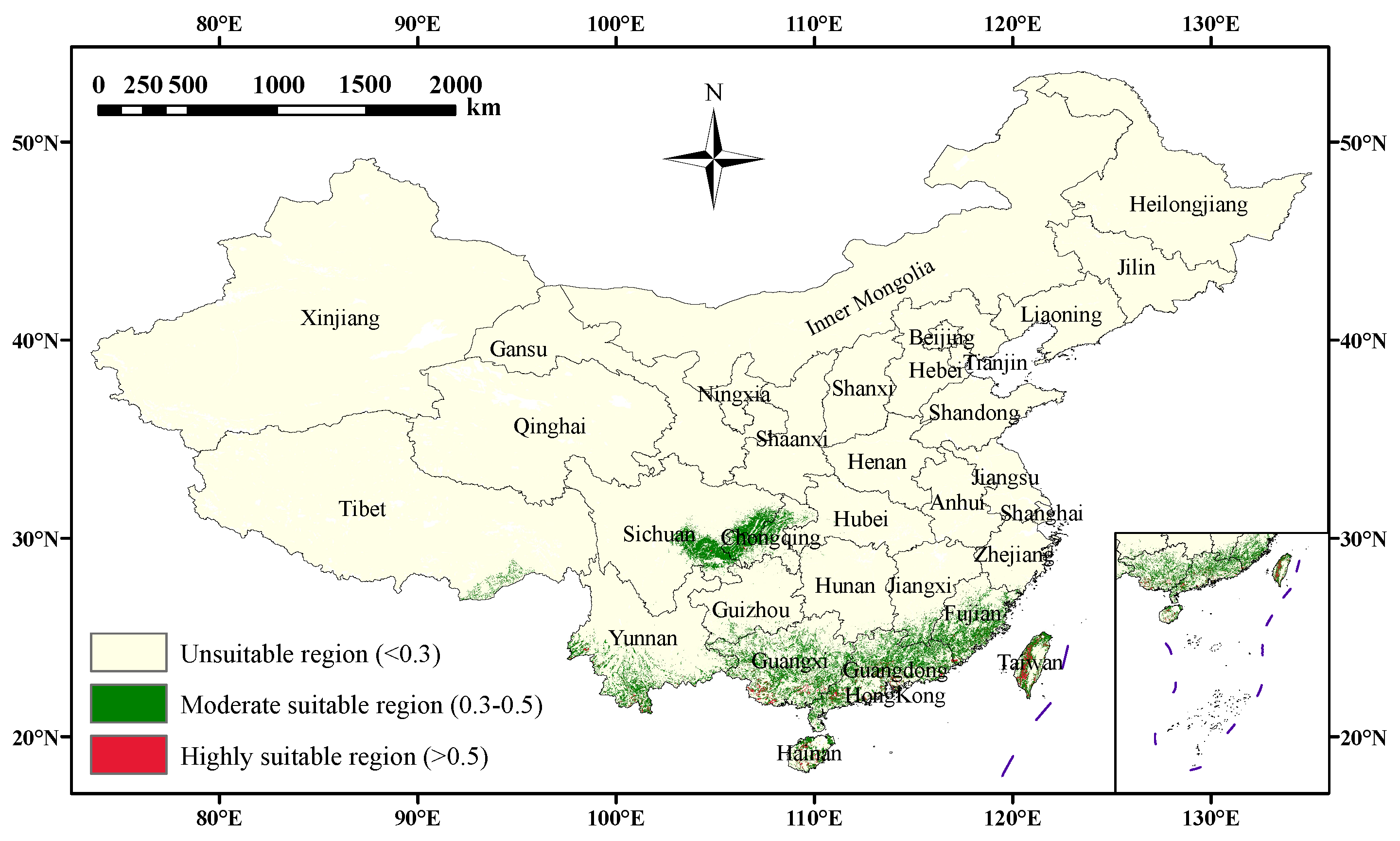
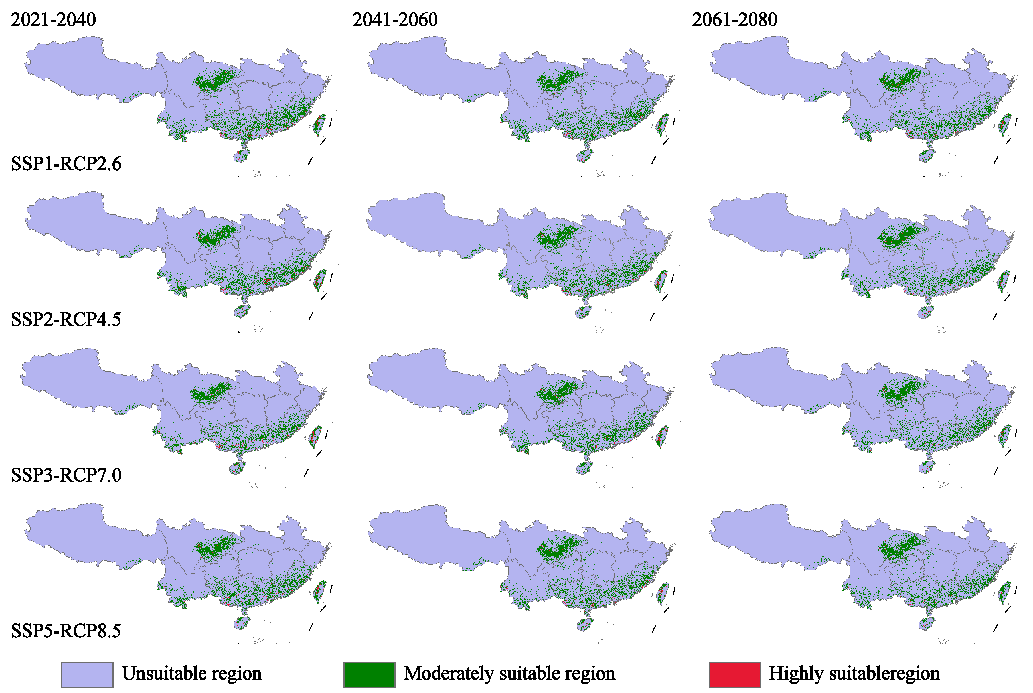
3.3. Current and Future Potential Suitable Habitats under Climate Change Scenarios

The CHS model revealed that the current suitable habitats for D. latiflorus cover a total area of 28.95 × 10⁴ km2, primarily located in two regions: Southeast China (Guangdong 21.53%, Fujian 11.66%) and Southwestern China (Guangxi 20.09%, Sichuan 13.24%, Yunnan 11.13%, Chongqing 7.90%). Additionally, significant populations are found on China’s two largest islands, Taiwan (5.55%) and Hainan (3.13%) (Figure 5, Table 2, Table S3). The habitats classified as moderately and highly suitable are 26.71 × 10⁴ km2 and 2.24 × 10⁴ km2, respectively. Moderately suitable habitats are found predominantly in Guangdong (21.16%), Guangxi (19.88%), Sichuan (14.19%), Fujian (12.08%), and Yunnan (11.28%). Highly suitable habitats are concentrated in Guangdong (26.00%), Guangxi (22.61%), and Taiwan’s Central Mountain Range (22.17%) (Table S3). Notably, the suitable habitats of D. latiflorus are fragmented into numerous small, non-contiguous patches. This fragmentation results from the incorporation of high-precision landscape and soil data into the CHS model.
Under future scenarios, the projected suitable habitats for D. latiflorus are 29.21 × 10⁴ km2 in the 2030s, 29.21 × 10⁴ km2 in the 2050s, and 28.76 × 10⁴ km2 in the 2070s, based on the average of four SSP scenarios (Table 2). Moderately suitable habitats remain stable, while highly suitable habitats decrease significantly (Figure 6 and Figure 7a, Table 2). A northward habitat expansion is observed, extending to Guizhou and Hunan by the 2050s and 2070s. Concurrently, habitat contraction in Fujian, Guangdong, and Guangxi increases from the current period to the 2070s (Figure 7b and Figure 8). In summary, suitable habitats increase by the 2050s and then decrease by the 2070s, with a northward expansion and a concurrent contraction in the southern regions.
Climate change exerts a more significant impact on suitable habitats than temporal factors (Figure 7c,d, Table 2). As climate change intensifies, a significant portion of highly suitable habitats will shift to moderately suitable or even unsuitable regions. Low-emission scenarios (SSP1-RCP2.6 and SSP2-RCP4.5) show a general trend of habitat expansion. Conversely, high-emission scenarios (SSP3-RCP7.0 and SSP5-RCP8.5) result in habitat contraction. By the 2070s, Guangdong and Guangxi will experience the most substantial reductions, exceeding 50%, under high emission scenarios.

3.4. Core Shift and Low-Impact Areas under Climate Change Scenarios

The current suitable habitat centroid for D. latiflorus, as indicated by a black dot in Figure 9, was predicted to be in northern Guangxi (25.0601° N, 108.9484° E). Under future scenarios, the centroid shifts northeastward to the border of Guangxi, Hunan, and Guizhou. Although the predicted centroid locations for the 2070s are similar, the paths show diverse movement patterns influenced by different climate scenarios and environmental factors. Under low-emission scenarios, the elevation of the centroid show an upward trend, with the SSP2-RCP4.5 scenario projecting an increase up to 1000 m. Conversely, under high-emission scenarios, the elevation peaks in the 2050s before declining. Overall, the centroid of suitable habitats for D. latiflorus shifts northeastward and upward in future scenarios (Figure 9, Table S4).
The projected SSP-specific Low-Impact Areas (SSP-LIAs) varied across the four SSPs. Under the SSP1-RCP2.6 scenario, there was a slight increase in SSP-LIAs. However, as climatic severity increased (from SSP1-RCP2.6 to SSP5-RCP8.5), the SSP-LIAs consistently decreased from 29.28 × 10⁴ km2 to 25.02 × 10⁴ km2 (Table 3). The LIAs, derived from the overlapping SSP-LIAs, indicated that the Sichuan Basin and the western side of Taiwan’s Central Mountain Range will be less impacted by climate change, serving as continuous refuges for D. latiflorus growth (Figure 10a,c). Additionally, climate change exacerbated the fragmentation of LIAs, causing the LIAs in Guangxi, Guangdong, Fujian, and Yunnan to retreat and concentrate at higher elevations (Figure 10b,c).

4. Discussion

4.1. Key Climate, Soil, and Landscape Factors Shaping Suitable Habitats

Species distribution is influenced by a combination of abiotic factors such as climate, topography, soil properties, and human activities, as well as biotic factors [15]. Among these abiotic factors, the hydro-thermal environment is critical in determining spatial distribution [65,83]. The present study identified annual mean temperature (Bio1) as the primary climatic variable influencing species spatial distribution (Figure 3b). The joint effect of annual precipitation (Bio12) with Bio1 has the greatest impact on the spatial distribution of Ma bamboo (Figure 3c).
Temperature regulates bamboo shoot germination and emergence [4,84]. Elevated temperatures, specifically those surpassing a potential warming threshold of 3 °C above present-day conditions, may substantially decrease the survival rates of bamboo [85]. This reduction is likely due to the adverse impact on shoot bud differentiation [86]. Our findings indicate that the moderately and highly suitable habitats for D. latiflorus are mainly concentrated in the southern subtropical zone (20–25° N) under current climate conditions (Figure 5), at a lower latitude than previously reported [4]. This discrepancy is attributed to the optimal mean annual temperature for D. latiflorus, which is 20–25 °C, higher than that for other bamboo species (Figure 3c). Furthermore, the high mean annual temperature in the Sichuan Basin supports dense and continuous bamboo forests despite its higher latitude.
Likewise, precipitation is essential for bamboo forest growth, particularly considering its joint effect with temperature constraints [4,87]. The amount of rainfall during the sprouting period of bamboo shoots in autumn directly impacts the number of shoots that will emerge in the following year. Once germination occurs in the spring, significant water is required to support the meristematic growth of internode tissues. Our study found that annual precipitation exceeding 1053 mm greatly enhances the survival probability of D. latiflorus, given that the temperature conditions are suitable for growth. The precipitation gradient from the subtropical monsoon climate results in a gradual decline in the moderately and highly suitable habitats from the southeast coast to the southwest. The rainfall brought by the southwest monsoon designates the Sichuan Basin as a primary distribution area for D. latiflorus.
Soil provides essential space and nutrients for plants’ survival while also imposing constraints on their distribution [46]. Our soil EM analysis identified the cation exchange capacity in the 20–40 cm soil layer (CECc 20–40 cm) as the key factor influencing the distribution of D. latiflorus (Figure 3a). The optimal CECc 20–40 cm, less than 40 cmolc/kg (Figure 3b), is relatively high and aligns with field observations that D. latiflorus thrives in soils with high cation exchange capacity. This high CEC indicates a soil’s ability to retain essential nutrients, providing a stable supply crucial for D. latiflorus growth. Therefore, high CEC is a key determinant of the optimal growth and distribution of D. latiflorus, highlighting the importance of soil nutrient retention capacity in supporting its physiological needs.
Landscape factors, including topography (e.g., elevation, slope, aspect) and surface texture (e.g., vegetation and land use), significantly influence plant species distributions by affecting the redistribution of hydro-thermal environments [15,16,88]. The response curve for vegetation indicated four suitable vegetation types for D. latiflorus. The optimal vegetation types were tri-annual crop fields, evergreen fruit orchards, and economic forests. The response curve for elevation showed that D. latiflorus thrives at elevations between 20 and 625 m, with the highest probability of presence at around 198 m (Figure 4, Table 1). However, the contribution of slope and aspect to the model was minimal, at only 2.4% and 1.9%, respectively. This aligns with field observations, where D. latiflorus grows without significant limitations from slope and aspect exposure.

4.2. Climate Change Driving Species Migration Trends

The spatial distribution of species is influenced by various biotic and abiotic factors, with climate change being a major determinant of large-scale distribution patterns [89]. Our analysis revealed that over three future periods, the suitable habitats of D. latiflorus showed a pattern of expansion followed by contraction compared to the current situation (Figure 7d). The contraction in suitable habitats for D. latiflorus is attributed to hydro-thermal variations due to climate change. These changes enhance drought stress and reduce soil moisture, thereby inhibiting plant survival, growth, and reproduction [65].
In response to climate change, species may adapt through phenological changes (timing-related, such as changes in flowering or breeding times) and/or physiological changes (acclimation, such as altering photosynthetic rates or water retention) [15,90], or migrate to higher latitudes or elevations to avoid warming temperatures and reduced precipitation [91]. By extracting the latitude and elevation information of each grid in the projected suitable habitats, the mean of each future scenario indicates that climate change will cause a shift in the suitable habitats for D. latiflorus in both latitude and elevation. This migration to higher latitudes and elevations becomes more pronounced with increased emissions across three future periods (Figure 11). This aligns with the findings of Li et al. [4], who projected that global warming would drive the northward migration of potential distribution areas for bamboo forests in China.
Increasing temperatures and decreasing precipitation tend to drive species to higher elevations rather than higher latitudes due to habitat fragmentation, which limits lateral migration [65]. Additionally, high elevations and high altitudes are predicted to experience the most rapid climate change, posing further threats to species’ suitable habitats [92]. As elevation increases, the available habitats for species migration decrease sharply, eventually leading to large-scale habitat contraction [93,94]. Consequently, populations in these habitats may become isolated to scattered stands. This isolation reduces gene flow between populations, resulting in genetic bottlenecks and decreased genetic diversity. Such genetic isolation compromises the adaptive potential of species to changing environmental conditions, elevating the risk of regional extinction as populations become less resilient to climatic and other environmental stresses. However, isolated small populations may also evolve rapidly and independently, potentially increasing genetic diversity through different selective pressures and genetic drift, which can lead to unique adaptations.
Fortunately, the significant impact of human activities on ecosystems has facilitated the widespread practice of human-mediated species migration. This phenomenon is especially prevalent among plants with high ornamental and economic value. Such interventions play a crucial role in overcoming the challenges associated with lateral migration [95]. By intentionally relocating these species to more favorable environments, humans can mitigate the adverse effects of climate change and habitat fragmentation. This proactive approach not only aids in the conservation of biodiversity but also ensures the continued ecological and economic benefits provided by these valuable plant species.

4.3. Development and Conservation Management of Germplasm Resources

D. latiflorus, a fast-growing woody grass with significant ecological and economic value, is suitable for cultivation in southern China [45,51]. Our study predicts that regions such as eastern Sichuan, western Chongqing, Fujian, Guangdong, Guangxi, western Taiwan, Hainan, and southern Yunnan will be less impacted by climate change (Figure 5 and Figure 7), making them ideal for increased D. latiflorus planting. Future planting efforts should focus on northern Sichuan and Chongqing to mitigate the effects of climate change (Figure 10).
To address climate change challenges, conservation strategies should include establishing botanical gardens and core germplasm through seedling transplantation and cultivation to preserve genetic diversity and ensure resource availability. These botanical gardens can serve as refuges for endangered species, providing controlled environments that mimic natural habitats and supporting ongoing research and education efforts.
Identifying suitable areas for these conservation efforts is crucial for effective management. This involves comprehensive site assessments to determine the optimal conditions for growth and survival, considering factors such as climate stability, soil quality, and accessibility. Collaboration with local communities and stakeholders is essential to ensure the sustainability and success of development and conservation initiatives. Furthermore, integrating advanced technologies such as Geographic Information Systems (GIS) and remote sensing can enhance the precision of habitat mapping and monitoring, allowing for adaptive management practices that respond to changing environmental conditions. This proactive approach not only aids in the conservation of D. latiflorus, but also contributes to the broader goal of preserving biodiversity and ecosystem services.
This comprehensive strategy ensures the long-term viability and ecological contributions of D. latiflorus, securing its benefits for future generations. Through these efforts, we can safeguard the ecological integrity of D. latiflorus forests and the diverse species they support, maintaining their critical role in global carbon sequestration and environmental health.

4.4. Model Rationality and Limitations

Species’ suitable habitats are shaped by a variety of biotic and abiotic factors [65]. To enhance the realism of our predictions, we built a CHS model by integrating climate, soil, and landscape variables, following established methodologies [14,15,16,46,47]. Additionally, to minimize model selection bias, we applied an ensemble model (EM) strategy for each variable category. After filtering for algorithmic and single-model performance (TSS ≥ 0.7, AUC ≥ 0.9), our EMs demonstrated excellent performance. Therefore, the species distribution models (SDMs) and CHS model results are considered adequate for predicting potential suitable habitats for D. latiflorus.
This study focused solely on the influence of abiotic factors such as climate, soil, topography, vegetation, and land use on species distribution. However, in reality, species distribution is also influenced by biotic factors like competition, parasitism, and predation [96]. Addressing these factors requires more complex and integrated SDMs, highlighting a critical direction for future model development [97]. Moreover, variables such as UV-B radiation, soil, vegetation, and land use were assumed to be constant in all future scenarios due to data limitations. These variables may not remain unchanged over the extended period from the present to the 2070s.
Another limitation of this study is that it did not account for migration rates, assuming instead that species have unlimited dispersal capabilities to move to any projected suitable habitats. This assumption introduces a degree of uncertainty in our predictions. Future research should aim to determine the migration rates of D. latiflorus to enhance prediction accuracy [98,99]. Despite these limitations, our study can provide a valuable insight into how climate, soil, and landscape factors influence the suitable habitats of D. latiflorus in China and the future changes in distribution patterns under climate change.

5. Conclusions

The present study developed a comprehensive habitat suitability (CHS) model integrating bioclimatic, UV-B radiation, soil attribute, topographical, vegetation, and land-use factors to project the suitable habitats and distribution dynamics of D. latiflorus in response to climate change. The projected current suitable habitats of D. latiflorus cover 28.95 × 10⁴ km2, primarily located in South China and the Sichuan Basin, including Sichuan, Chongqing, Fujian, Guangdong, Guangxi, Taiwan, Hainan, and Yunnan. The most influential factors were the joint effect of annual mean temperature (Bio1) and annual precipitation (Bio12), cation exchange capacity in the 20–40 cm soil layer (CECc 20–40 cm), vegetation type, and elevation.
Future scenarios show an initial slight expansion of suitable habitats followed by a contraction trend, along with a northward shift in latitude and migration to higher elevations compared to the current distribution. The Sichuan Basin (Sichuan–Chongqing border) was identified as a climatically stable area that could serve as a focal point for germplasm development and conservation.
Our findings underscore the critical impact of climate change on D. latiflorus distribution, highlighting the need for proactive development and conservation strategies. The stability of the Sichuan Basin offers a key opportunity for germplasm development and conservation, ensuring the species’ long-term survival and its ecological and economic contributions. Decision makers should prioritize these stable regions and consider habitat shifts to mitigate climate change effects, thereby preserving the biodiversity, ecological benefits, and industrial uses of D. latiflorus forests.

Supplementary Materials

The following supporting information can be downloaded at: https://www.mdpi.com/article/10.3390/f15081321/s1, Figure S1: Variable selection using PCA and Pearson correlation; Figure S2: Evaluation scores of climate and soil ensemble models Using TSS and AUC metrics; Figure S3: Distribution of models, non-statistically significant models, and selected models based on AICc and omission rate values; Figure S4: Single response curves of climate EM; Figure S5: Bivariate response curves of climate EM; Figure S6: Single response curves of soil EM; Table S1: Filtered species presence data and environmental variables for SDM modeling; Table S2: Description and selection of environmental variables; Table S3: Areas and percentages of habitat suitability distributions by province for D. latiflorus under different scenarios; Table S4: Elevation, latitude, and longitude of core potential suitable areas for D. latiflorus from current to future climate scenarios.

Author Contributions

Conceptualization, L.-J.C.; methodology, L.-J.C.; software, Y.-Q.X.; validation, L.-J.C. and Y.-Q.X.; formal analysis, Y.-Q.X.; investigation, L.-J.C., Y.-Q.X., T.-Y.H., L.-Y.C., J.-D.R. and L.-G.C.; resources, L.-J.C., Y.-Q.X., T.-Y.H., L.-Y.C., J.-D.R. and L.-G.C.; data curation, Y.-Q.X.; writing—original draft preparation, L.-J.C. and Y.-Q.X.; writing—review and editing, L.-J.C., Y.-Q.X., T.-Y.H., L.-Y.C., J.-D.R., L.-G.C. and Y.-S.Z.; visualization, Y.-Q.X.; supervision, Y.-S.Z.; project administration, Y.-S.Z.; funding acquisition, Y.-S.Z. All authors have read and agreed to the published version of the manuscript.

Funding

This research was funded by the National Key R&D Program of China (Grant No. 2023YFD2201201).

Data Availability Statement

The original contributions presented in this study are included in the Supplementary Materials. Further inquiries can be directed to the corresponding author.

Acknowledgments

We would like to express our deepest gratitude to all the members who participated in this research. We extend our sincere thanks to Hui Huang for providing expert technical support in data processing and analysis, which was instrumental in the successful completion of this article.

Conflicts of Interest

The authors declare no conflicts of interest.

References

  1. Zhou, G.; Meng, C.; Jiang, P.; Xu, Q. Review of Carbon Fixation in Bamboo Forests in China. Bot. Rev. 2011, 77, 262–270. [Google Scholar] [CrossRef]
  2. Chen, Y.; Jiang, H.; Zhou, G.; Yang, S.; Chen, J. Estimation of CO2 Fluxes and Its Seasonal Variations from the Effective Management Lei Bamboo (Phyllostachys violascens). Acta Ecol. Sin. 2013, 33, 3434–3444. [Google Scholar] [CrossRef]
  3. Liu, Y.; Zhou, G.; Du, H.; Berninger, F.; Mao, F.; Li, X.; Chen, L.; Cui, L.; Li, Y.; Zhu, D.; et al. Response of Carbon Uptake to Abiotic and Biotic Drivers in an Intensively Managed Lei Bamboo Forest. J. Environ. Manag. 2018, 223, 713–722. [Google Scholar] [CrossRef] [PubMed]
  4. Li, X.; Mao, F.; Du, H.; Zhou, G.; Xing, L.; Liu, T.; Han, N.; Liu, Y.; Zhu, D.; Zheng, J.; et al. Spatiotemporal Evolution and Impacts of Climate Change on Bamboo Distribution in China. J. Environ. Manag. 2019, 248, 109265. [Google Scholar] [CrossRef] [PubMed]
  5. China Bamboo Industry Association. National Bamboo Industry Development Plan (2021–2030); Technical Report; China Bamboo Industry Association: Beijing, China, 2022. [Google Scholar]
  6. Tuanmu, M.N.; Viña, A.; Winkler, J.A.; Li, Y.; Xu, W.; Ouyang, Z.; Liu, J. Climate-Change Impacts on Understorey Bamboo Species and Giant Pandas in China’s Qinling Mountains. Nat. Clim. Chang. 2013, 3, 249–253. [Google Scholar] [CrossRef]
  7. Zhou, W. An Analysis of the influence of precipitation on the growth of bamboo forest. J. Bamboo Res. 1991, 9, 33–39. [Google Scholar]
  8. Janzen, D.H. Why Bamboos Wait so Long to Flower. Annu. Rev. Ecol. Syst. 1976, 7, 347–391. [Google Scholar] [CrossRef]
  9. Taylor, A.H.; Reid, D.G.; Zisheng, Q.; Jinchu, H. Spatial Patterns and Environmental Associates of Bamboo (Bashania fangiana Yi) after Mass-Flowering in Southwestern China. Bull. Torrey Bot. Club 1991, 118, 247. [Google Scholar] [CrossRef]
  10. Taylor, A.H.; Zisheng, Q. Structure and Dynamics of Bamboos in the Wolong Natural Reserve, China. Am. J. Bot. 1993, 80, 375–384. [Google Scholar] [CrossRef]
  11. Cai, B.; Jin, H. Biological characteristics of bamboo and it application in scenic gardening. World Bamboo Ratt. 2010, 8, 39–43. [Google Scholar]
  12. Anderson, R.P. A Framework for Using Niche Models to Estimate Impacts of Climate Change on Species Distributions. Ann. N. Y. Acad. Sci. 2013, 1297, 8–28. [Google Scholar] [CrossRef]
  13. Elith, J.; Graham, C.H.; Anderson, R.P.; Dudík, M.; Ferrier, S.; Guisan, A.; Hijmans, R.J.; Huettmann, F.; Leathwick, J.R.; Lehmann, A.; et al. Novel Methods Improve Prediction of Species’ Distributions from Occurrence Data. Ecography 2006, 29, 129–151. [Google Scholar] [CrossRef]
  14. Guo, Y.; Li, X.; Zhao, Z.; Nawaz, Z. Predicting the Impacts of Climate Change, Soils and Vegetation Types on the Geographic Distribution of Polyporus umbellatus in China. Sci. Total Environ. 2019, 648, 1–11. [Google Scholar] [CrossRef] [PubMed]
  15. Wu, Y.M.; Shen, X.L.; Tong, L.; Lei, F.W.; Mu, X.Y.; Zhang, Z.X. Impact of Past and Future Climate Change on the Potential Distribution of an Endangered Montane Shrub Lonicera oblata and Its Conservation Implications. Forests 2021, 12, 125. [Google Scholar] [CrossRef]
  16. Zhao, Z.; Guo, Y.; Wei, H.; Ran, Q.; Liu, J.; Zhang, Q.; Gu, W. Potential Distribution of Notopterygium incisum Ting Ex H. T. Chang and Its Predicted Responses to Climate Change Based on a Comprehensive Habitat Suitability Model. Ecol. Evol. 2020, 10, 3004–3016. [Google Scholar] [CrossRef]
  17. Marmion, M.; Luoto, M.; Heikkinen, R.K.; Thuiller, W. The Performance of State-of-the-Art Modelling Techniques Depends on Geographical Distribution of Species. Ecol. Model. 2009, 220, 3512–3520. [Google Scholar] [CrossRef]
  18. Naimi, B.; Araújo, M.B. Sdm: A Reproducible and Extensible R Platform for Species Distribution Modelling. Ecography 2016, 39, 368–375. [Google Scholar] [CrossRef]
  19. Cobos, M.E.; Peterson, A.T.; Barve, N.; Osorio-Olvera, L. Kuenm: An R Package for Detailed Development of Ecological Niche Models Using Maxent. PeerJ 2019, 7, e6281. [Google Scholar] [CrossRef]
  20. Thuiller, W.; Georges, D.; Gueguen, M.; Engler, R.; Breiner, F.; Lafourcade, B.; Patin, R.; Blancheteau, H. Biomod2: Ensemble Platform for Species Distribution Modeling; R Core Team: Vienna, Austria, 2024. [Google Scholar]
  21. Segurado, P.; Araújo, M.B. An Evaluation of Methods for Modelling Species Distributions. J. Biogeogr. 2004, 31, 1555–1568. [Google Scholar] [CrossRef]
  22. Thuiller, W.; Araújo, M.B.; Lavorel, S. Generalized Models vs. Classification Tree Analysis: Predicting Spatial Distributions of Plant Species at Different Scales. J. Veg. Sci. 2003, 14, 669–680. [Google Scholar] [CrossRef]
  23. Basile, M.; Valerio, F.; Balestrieri, R.; Posillico, M.; Bucci, R.; Altea, T.; Cinti, B.D.; Matteucci, G. Patchiness of Forest Landscape Can Predict Species Distribution Better than Abundance: The Case of a Forest-Dwelling Passerine, the Short-Toed Treecreeper, in Central Italy. PeerJ 2016, 4, e2398. [Google Scholar] [CrossRef] [PubMed]
  24. Muñoz-Mas, R.; Papadaki, C.; Martínez-Capel, F.; Zogaris, S.; Ntoanidis, L.; Dimitriou, E. Generalized Additive and Fuzzy Models in Environmental Flow Assessment: A Comparison Employing the West Balkan Trout (Salmo farioides; Karaman, 1938). Ecol. Eng. 2016, 91, 365–377. [Google Scholar] [CrossRef]
  25. Moisen, G.G.; Freeman, E.A.; Blackard, J.A.; Frescino, T.S.; Zimmermann, N.E.; Edwards, T.C. Predicting Tree Species Presence and Basal Area in Utah: A Comparison of Stochastic Gradient Boosting, Generalized Additive Models, and Tree-Based Methods. Ecol. Model. 2006, 199, 176–187. [Google Scholar] [CrossRef]
  26. Lopatin, J.; Dolos, K.; Hernández, H.J.; Galleguillos, M.; Fassnacht, F.E. Comparing Generalized Linear Models and Random Forest to Model Vascular Plant Species Richness Using LiDAR Data in a Natural Forest in Central Chile. Remote Sens. Environ. 2016, 173, 200–210. [Google Scholar] [CrossRef]
  27. Friedman, J.H. Multivariate Adaptive Regression Splines. Ann. Stat. 1991, 19, 1–67. [Google Scholar] [CrossRef]
  28. Phillips, S.J.; Anderson, R.P.; Schapire, R.E. Maximum Entropy Modeling of Species Geographic Distributions. Ecol. Model. 2006, 190, 231–259. [Google Scholar] [CrossRef]
  29. Phillips, S.J.; Anderson, R.P.; Dudík, M.; Schapire, R.E.; Blair, M.E. Opening the Black Box: An Open-source Release of Maxent. Ecography 2017, 40, 887–893. [Google Scholar] [CrossRef]
  30. Mi, C.; Huettmann, F.; Guo, Y.; Han, X.; Wen, L. Why Choose Random Forest to Predict Rare Species Distribution with Few Samples in Large Undersampled Areas? Three Asian Crane Species Models Provide Supporting Evidence. PeerJ 2017, 5, e2849. [Google Scholar] [CrossRef]
  31. Booth, T.H.; Nix, H.A.; Busby, J.R.; Hutchinson, M.F. Bioclim: The First Species Distribution Modelling Package, Its Early Applications and Relevance to Most Current MaxEnt Studies. Divers. Distrib. 2014, 20, 1–9. [Google Scholar] [CrossRef]
  32. Chen, T.; Guestrin, C. XGBoost: A Scalable Tree Boosting System. In Proceedings of the 22nd ACM SIGKDD International Conference on Knowledge Discovery and Data Mining, San Francisco, CA, USA, 13–17 August 2016; pp. 785–794. [Google Scholar] [CrossRef]
  33. Zhang, L.; Liu, S.; Sun, P.; Wang, T.; Wang, G.; Zhang, X.; Wang, L. Consensus Forecasting of Species Distributions: The Effects of Niche Model Performance and Niche Properties. PLoS ONE 2015, 10, e0120056. [Google Scholar] [CrossRef]
  34. Strubbe, D.; Jackson, H.; Groombridge, J.; Matthysen, E. Invasion Success of a Global Avian Invader Is Explained by Within-Taxon Niche Structure and Association with Humans in the Native Range. Divers. Distrib. 2015, 21, 675–685. [Google Scholar] [CrossRef]
  35. Thuiller, W.; Lafourcade, B.; Engler, R.; Araújo, M.B. BIOMOD—A Platform for Ensemble Forecasting of Species Distributions. Ecography 2009, 32, 369–373. [Google Scholar] [CrossRef]
  36. Burnham, K.P.; Anderson, D.R.; Anderson, D.R. Model Selection and Multimodel Inference: A Practical Information-Theoretic Approach, 2nd ed.; Springer: New York, NY, USA, 2010. [Google Scholar]
  37. Guisan, A.; Thuiller, W.; Zimmermann, N.E. Habitat Suitability and Distribution Models: With Applications in R, 1st ed.; Cambridge University Press: Cambridge, UK, 2017. [Google Scholar] [CrossRef]
  38. Shinohara, Y.; Misumi, Y.; Kubota, T.; Nanko, K. Characteristics of Soil Erosion in a Moso-Bamboo Forest of Western Japan: Comparison with a Broadleaved Forest and a Coniferous Forest. CATENA 2019, 172, 451–460. [Google Scholar] [CrossRef]
  39. Liu, Y.H.; Yen, T.M. Assessing Aboveground Carbon Storage Capacity in Bamboo Plantations with Various Species Related to Its Affecting Factors across Taiwan. For. Ecol. Manag. 2021, 481, 118745. [Google Scholar] [CrossRef]
  40. Ramakrishnan, M.; Yrjälä, K.; Vinod, K.K.; Sharma, A.; Cho, J.; Satheesh, V.; Zhou, M. Genetics and Genomics of Moso Bamboo (Phyllostachys edulis): Current Status, Future Challenges, and Biotechnological Opportunities toward a Sustainable Bamboo Industry. Food Energy Secur. 2020, 9, e229. [Google Scholar] [CrossRef]
  41. Choudhury, D.; Sahu, J.K.; Sharma, G.D. Value Addition to Bamboo Shoots: A Review. J. Food Sci. Technol. 2012, 49, 407–414. [Google Scholar] [CrossRef] [PubMed]
  42. Noremylia, M.B.; Aufa, A.N.; Ismail, Z.; Hassan, M.Z. An Overview of the Potential Usage of Bamboo Plants in Medical Field. In Bamboo Science and Technology; Palombini, F.L., Nogueira, F.M., Eds.; Springer Nature: Singapore, 2023; pp. 55–66. [Google Scholar] [CrossRef]
  43. Taylor, A.H.; Jinyan, H.; ShiQiang, Z. Canopy Tree Development and Undergrowth Bamboo Dynamics in Old-Growth Abies–Betula Forests in Southwestern China: A 12-Year Study. For. Ecol. Manag. 2004, 200, 347–360. [Google Scholar] [CrossRef]
  44. Fan, L.; Zhao, T.; Tarin, M.W.K.; Han, Y.; Hu, W.; Rong, J.; He, T.; Zheng, Y. Effect of Various Mulch Materials on Chemical Properties of Soil, Leaves and Shoot Characteristics in Dendrocalamus latiflorus Munro Forests. Plants 2021, 10, 2302. [Google Scholar] [CrossRef]
  45. Deng, C.; Li, K.J.; Xiang, P.Z. Study on the Distribution Pattern of Dendrocalamus latiflorus in China Based on the Maximum Entropy Model (MaxEnt) and Geographic Information System (GIS). Environ. Ecol. 2023, 5, 69–74. [Google Scholar]
  46. Liu, J.; Yang, Y.; Wei, H.; Zhang, Q.; Zhang, X.; Zhang, X.; Gu, W. Assessing Habitat Suitability of Parasitic Plant Cistanche deserticola in Northwest China under Future Climate Scenarios. Forests 2019, 10, 823. [Google Scholar] [CrossRef]
  47. Guo, Y.; Li, X.; Zhao, Z.; Wei, H.; Gao, B.; Gu, W. Prediction of the Potential Geographic Distribution of the Ectomycorrhizal Mushroom Tricholoma matsutake under Multiple Climate Change Scenarios. Sci. Rep. 2017, 7, 46221. [Google Scholar] [CrossRef]
  48. Zhang, X.M.; Zhao, L.; Larson-Rabin, Z.; Li, D.Z.; Guo, Z.H. De Novo Sequencing and Characterization of the Floral Transcriptome of Dendrocalamus latiflorus (Poaceae: Bambusoideae). PLoS ONE 2012, 7, e42082. [Google Scholar] [CrossRef]
  49. Wu, J.; Zheng, J.; Xia, X.; Kan, J. Purification and Structural Identification of Polysaccharides from Bamboo Shoots (Dendrocalamus latiflorus). Int. J. Mol. Sci. 2015, 16, 15560–15577. [Google Scholar] [CrossRef]
  50. Wu, F.H.; Kan, D.P.; Lee, S.B.; Daniell, H.; Lee, Y.W.; Lin, C.C.; Lin, N.S.; Lin, C.S. Complete Nucleotide Sequence of Dendrocalamus latiflorus and Bambusa oldhamii Chloroplast Genomes. Tree Physiol. 2009, 29, 847–856. [Google Scholar] [CrossRef] [PubMed]
  51. Zheng, Y.; Yang, D.; Rong, J.; Chen, L.; Zhu, Q.; He, T.; Chen, L.; Ye, J.; Fan, L.; Gao, Y.; et al. Allele-Aware Chromosome-Scale Assembly of the Allopolyploid Genome of Hexaploid Ma Bamboo (Dendrocalamus latiflorus Munro). J. Integr. Plant Biol. 2022, 64, 649–670. [Google Scholar] [CrossRef]
  52. Ye, S.; Cai, C.; Ren, H.; Wang, W.; Xiang, M.; Tang, X.; Zhu, C.; Yin, T.; Zhang, L.; Zhu, Q. An Efficient Plant Regeneration and Transformation System of Ma Bamboo (Dendrocalamus latiflorus Munro) Started from Young Shoot as Explant. Front. Plant Sci. 2017, 8, 1298. [Google Scholar] [CrossRef]
  53. Yen, T.M.; Sun, P.K.; Li, L.E. Predicting Aboveground Biomass and Carbon Storage for Ma Bamboo (Dendrocalamus latiflorus Munro) Plantations. Forests 2023, 14, 854. [Google Scholar] [CrossRef]
  54. Sampaio, U.M.; da Silva, M.F.; Goldbeck, R.; Clerici, M.T.P.S. Technological and Prebiotic Aspects of Young Bamboo Culm Flour (Dendrocalamus latiflorus) Combined with Rice Flour to Produce Healthy Extruded Products. Food Res. Int. 2023, 165, 112482. [Google Scholar] [CrossRef]
  55. Cui, L.; Du, H.; Zhou, G.; Li, X.; Mao, F.; Xu, X.; Fan, W.; Li, Y.; Zhu, D.; Liu, T.; et al. Combination of Decision Tree and Mixed Pixel Decomposition for Extracting Bamboo Forest Information in China. Natl. Remote. Sens. Bull. 2021, 23, 166–176. [Google Scholar] [CrossRef]
  56. Li, Y.; Han, N.; Li, X.; Du, H.; Mao, F.; Cui, L.; Liu, T.; Xing, L. Spatiotemporal Estimation of Bamboo Forest Aboveground Carbon Storage Based on Landsat Data in Zhejiang, China. Remote Sens. 2018, 10, 898. [Google Scholar] [CrossRef]
  57. Brown, J.L.; Bennett, J.R.; French, C.M. SDMtoolbox 2.0: The next Generation Python-Based GIS Toolkit for Landscape Genetic, Biogeographic and Species Distribution Model Analyses. PeerJ 2017, 5, e4095. [Google Scholar] [CrossRef] [PubMed]
  58. Almasieh, K.; Mirghazanfari, S.M.; Mahmoodi, S. Biodiversity Hotspots for Modeled Habitat Patches and Corridors of Species Richness and Threatened Species of Reptiles in Central Iran. Eur. J. Wildl. Res. 2019, 65, 92. [Google Scholar] [CrossRef]
  59. Zhang, L.; Liu, S.; Sun, P.; Wang, T.; Wang, G.; Wang, L.; Zhang, X. Using DEM to Predict Abies faxoniana and Quercus aquifolioides Distributions in the Upstream Catchment Basin of the Min River in Southwest China. Ecol. Indic. 2016, 69, 91–99. [Google Scholar] [CrossRef]
  60. Elith, J.; Leathwick, J.R. Species Distribution Models: Ecological Explanation and Prediction across Space and Time. Annu. Rev. Ecol. Evol. Syst. 2009, 40, 677–697. [Google Scholar] [CrossRef]
  61. Zimmermann, N.E.; Edwards, T.C.; Graham, C.H.; Pearman, P.B.; Svenning, J.C. New Trends in Species Distribution Modelling. Ecography 2010, 33, 985–989. [Google Scholar] [CrossRef]
  62. Fick, S.E.; Hijmans, R.J. WorldClim 2: New 1-km Spatial Resolution Climate Surfaces for Global Land Areas. Int. J. Climatol. 2017, 37, 4302–4315. [Google Scholar] [CrossRef]
  63. Mu, C.; Guo, X.; Chen, Y. Impact of Global Climate Change on the Distribution Range and Niche Dynamics of Eleutherodactylus Planirostrish in China. Biology 2022, 11, 588. [Google Scholar] [CrossRef]
  64. Lv, Z.; Li, D. The Potential Distribution of Juniperus rigida Sieb. et Zucc. Vary Diversely in China under the Stringent and High GHG Emission Scenarios Combined Bioclimatic, Soil, and Topographic Factors. Forests 2021, 12, 1140. [Google Scholar] [CrossRef]
  65. Sun, S.; Zhang, Y.; Huang, D.; Wang, H.; Cao, Q.; Fan, P.; Yang, N.; Zheng, P.; Wang, R. The Effect of Climate Change on the Richness Distribution Pattern of Oaks (Quercus L.) in China. Sci. Total Environ. 2020, 744, 140786. [Google Scholar] [CrossRef]
  66. Beckmann, M.; Václavík, T.; Manceur, A.M.; Šprtová, L.; Von Wehrden, H.; Welk, E.; Cord, A.F. glUV: A Global UV-B Radiation Data Set for Macroecological Studies. Methods Ecol. Evol. 2014, 5, 372–383. [Google Scholar] [CrossRef]
  67. Zhu, M.; Zhang, C.; Zhang, J.; Feng, Q. The Grid Data of Soil Properties Based on WISE30sec; Northwest Institute of Eco-Environment and Resources: Lanzhou, China, 2023. [Google Scholar] [CrossRef]
  68. Batjes, N. Harmonized Soil Property Values for Broad-Scale Modelling (WISE30sec) with Estimates of Global Soil Carbon Stocks. Geoderma 2016, 269, 61–68. [Google Scholar] [CrossRef]
  69. An, Y.; Zhou, B. Research on structure and biomechanics of bamboos underground system: A review. Chin. Agric. Sci. Bull. 2009, 25, 83–88. [Google Scholar]
  70. Tong, R.; Chen, Q.; Zhou, B.; Tang, Y.; An, Y.; Ge, X.; Cao, Y.; Yang, Z. Structure and Biomechanical Properties of Underground System of Moso Bamboo and Lei Bamboo. Acta Ecol. Sin. 2018, 40, 2242–2251. [Google Scholar] [CrossRef]
  71. Yamazaki, D.; Ikeshima, D.; Tawatari, R.; Yamaguchi, T.; O’Loughlin, F.; Neal, J.C.; Sampson, C.C.; Kanae, S.; Bates, P.D. A High-accuracy Map of Global Terrain Elevations. Geophys. Res. Lett. 2017, 44, 5844–5853. [Google Scholar] [CrossRef]
  72. Editorial Committee of Chinese Vegetation Map. 1:1 Million Vegetation Data Set in China; Northwest Institute of Eco-Environment and Resources: Lanzhou, China, 2023. [Google Scholar] [CrossRef]
  73. Youhua, R. Comprehensive Land Cover Dataset of China; Northwest Institute of Eco-Environment and Resources: Lanzhou, China, 2020. [Google Scholar] [CrossRef]
  74. Graham, M.H. Confronting Multicollinearity in Ecological Multiple Regression. Ecology 2003, 84, 2809–2815. [Google Scholar] [CrossRef]
  75. R Core Team. R: A Language and Environment for Statistical Computing; R Core Team: Vienna, Austria, 2022. [Google Scholar]
  76. Zhao, Q.; Mi, Z.Y.; Lu, C.; Zhang, X.F.; Chen, L.J.; Wang, S.Q.; Niu, J.F.; Wang, Z.Z. Predicting Potential Distribution of Ziziphus spinosa (Bunge) H.H. Hu Ex F.H. Chen in China under Climate Change Scenarios. Ecol. Evol. 2022, 12, e8629. [Google Scholar] [CrossRef] [PubMed]
  77. Zurell, D.; Franklin, J.; König, C.; Bouchet, P.J.; Dormann, C.F.; Elith, J.; Fandos, G.; Feng, X.; Guillera-Arroita, G.; Guisan, A.; et al. A Standard Protocol for Reporting Species Distribution Models. Ecography 2020, 43, 1261–1277. [Google Scholar] [CrossRef]
  78. Santos-Hernández, A.F.; Monterroso-Rivas, A.I.; Granados-Sánchez, D.; Villanueva-Morales, A.; Santacruz-Carrillo, M. Projections for Mexico’s Tropical Rainforests Considering Ecological Niche and Climate Change. Forests 2021, 12, 119. [Google Scholar] [CrossRef]
  79. Smith, A.B.; Godsoe, W.; Rodríguez-Sánchez, F.; Wang, H.H.; Warren, D. Niche Estimation above and below the Species Level. Trends Ecol. Evol. 2019, 34, 260–273. [Google Scholar] [CrossRef]
  80. Pan, J.; Fan, X.; Luo, S.; Zhang, Y.; Yao, S.; Guo, Q.; Qian, Z. Predicting the Potential Distribution of Two Varieties of Litsea coreana (Leopard-Skin Camphor) in China under Climate Change. Forests 2020, 11, 1159. [Google Scholar] [CrossRef]
  81. Zhao, Q.; Zhang, Y.; Li, W.N.; Hu, B.W.; Zou, J.B.; Wang, S.Q.; Niu, J.F.; Wang, Z.Z. Predicting the Potential Distribution of Perennial Plant Coptis chinensis Franch. in China under Multiple Climate Change Scenarios. Forests 2021, 12, 1464. [Google Scholar] [CrossRef]
  82. Elith, J.; Ferrier, S.; Huettmann, F.; Leathwick, J. The Evaluation Strip: A New and Robust Method for Plotting Predicted Responses from Species Distribution Models. Ecol. Model. 2005, 186, 280–289. [Google Scholar] [CrossRef]
  83. Punyasena, S.W.; Eshel, G.; McElwain, J.C. The Influence of Climate on the Spatial Patterning of Neotropical Plant Families. J. Biogeogr. 2008, 35, 117–130. [Google Scholar] [CrossRef]
  84. Zhang, Y. A Study of the Effects of Climatic Fluctuation on Chinese Fir and Bamboo Ecological Environment in Subtropical Regions in China. Q. J. Appl. Meteorol. 1995, 6, 75–82. [Google Scholar]
  85. Yang, H.; Zhang, D.; Winkler, J.A.; Huang, Q.; Zhang, Y.; Wu, P.; Liu, J.; Ouyang, Z.; Xu, W.; Chen, X.; et al. Field Experiment Reveals Complex Warming Impacts on Giant Pandas’ Bamboo Diet. Biol. Conserv. 2024, 294, 110635. [Google Scholar] [CrossRef]
  86. Ying-chun, L.; Qing-ping, Y.; Zi-wu, G.; Shuang-lin, C.; Jun-jing, H. Damage Characteristics of Phyllostachys edulis Stands under Continuous High Temperature and Drought. For. Res. 2015, 28, 646–653. [Google Scholar]
  87. Shi, P.; Preisler, H.K.; Quinn, B.K.; Zhao, J.; Huang, W.; Röll, A.; Cheng, X.; Li, H.; Hölscher, D. Precipitation Is the Most Crucial Factor Determining the Distribution of Moso Bamboo in Mainland China. Glob. Ecol. Conserv. 2020, 22, e00924. [Google Scholar] [CrossRef]
  88. Wang, J.; Wang, Y.; Feng, J.; Chen, C.; Chen, J.; Long, T.; Li, J.; Zang, R.; Li, J. Differential Responses to Climate and Land-Use Changes in Threatened Chinese Taxus Species. Forests 2019, 10, 766. [Google Scholar] [CrossRef]
  89. Pearson, R.G.; Dawson, T.P. Predicting the Impacts of Climate Change on the Distribution of Species: Are Bioclimate Envelope Models Useful? Glob. Ecol. Biogeogr. 2003, 12, 361–371. [Google Scholar] [CrossRef]
  90. Bertrand, R.; Lenoir, J.; Piedallu, C.; Riofrío-Dillon, G.; De Ruffray, P.; Vidal, C.; Pierrat, J.C.; Gégout, J.C. Changes in Plant Community Composition Lag behind Climate Warming in Lowland Forests. Nature 2011, 479, 517–520. [Google Scholar] [CrossRef]
  91. Root, T.L.; Price, J.T.; Hall, K.R.; Schneider, S.H.; Rosenzweig, C.; Pounds, J.A. Fingerprints of Global Warming on Wild Animals and Plants. Nature 2003, 421, 57–60. [Google Scholar] [CrossRef] [PubMed]
  92. Loarie, S.R.; Duffy, P.B.; Hamilton, H.; Asner, G.P.; Field, C.B.; Ackerly, D.D. The Velocity of Climate Change. Nature 2009, 462, 1052–1055. [Google Scholar] [CrossRef]
  93. Nogués-Bravo, D.; Araújo, M.; Errea, M.; Martínez-Rica, J. Exposure of Global Mountain Systems to Climate Warming during the 21st Century. Glob. Environ. Chang. 2007, 17, 420–428. [Google Scholar] [CrossRef]
  94. Dawson, T.P.; Jackson, S.T.; House, J.I.; Prentice, I.C.; Mace, G.M. Beyond Predictions: Biodiversity Conservation in a Changing Climate. Science 2011, 332, 53–58. [Google Scholar] [CrossRef] [PubMed]
  95. Bellard, C.; Bertelsmeier, C.; Leadley, P.; Thuiller, W.; Courchamp, F. Impacts of Climate Change on the Future of Biodiversity. Ecol. Lett. 2012, 15, 365–377. [Google Scholar] [CrossRef]
  96. Boulangeat, I.; Gravel, D.; Thuiller, W. Accounting for Dispersal and Biotic Interactions to Disentangle the Drivers of Species Distributions and Their Abundances. Ecol. Lett. 2012, 15, 584–593. [Google Scholar] [CrossRef]
  97. Kearney, M.; Porter, W. Mechanistic Niche Modelling: Combining Physiological and Spatial Data to Predict Species’ Ranges. Ecol. Lett. 2009, 12, 334–350. [Google Scholar] [CrossRef] [PubMed]
  98. Meier, E.S.; Lischke, H.; Schmatz, D.R.; Zimmermann, N.E. Climate, Competition and Connectivity Affect Future Migration and Ranges of European Trees. Glob. Ecol. Biogeogr. 2012, 21, 164–178. [Google Scholar] [CrossRef]
  99. Ohlemüller, R.; Gritti, E.S.; Sykes, M.T.; Thomas, C.D. Quantifying Components of Risk for European Woody Species under Climate Change. Glob. Chang. Biol. 2006, 12, 1788–1799. [Google Scholar] [CrossRef]
Figure 1. Methodological approaches for comprehensive habitat suitability evaluation.
Forests 15 01321 g001
Figure 2. Occurrence data (165 points) of D. latiflorus in China.
Forests 15 01321 g002
Figure 3. Variable importance and response curves of key climate and soil variables in the modeled distribution of D. latiflorus based on ensemble models. (a) Single variable importance of climate EM; (b) response curve of Bio1; (c) bivariate response curves of Bio1 and Bio12; (d) single variable importance of soil EM; (e) response curve of CECc 20–40 cm; (f) bivariate response curves of CECc 20–40 cm and ECEC 0–20 cm.
Forests 15 01321 g003
Figure 4. Response curves of key environmental variables for the modeled distribution of D. latiflorus using the MaxEnt algorithm. (a) Vegetation; (b) elevation.
Forests 15 01321 g004
Figure 5. Comprehensive habitat suitability area of D. latiflorus in the current period.
Forests 15 01321 g005
Figure 6. Areas of unsuitable, moderately suitable, and highly suitable regions for D. latiflorus under different scenarios.
Forests 15 01321 g006
Figure 7. Changes in areas and patterns of D. latiflorus from current to future scenarios. (a) Percentage of habitats with different suitability under future scenarios; (b) percentage of pattern changes under future scenarios; (c) area changes under different GHG emission scenarios; (d) area changes across different periods.
Forests 15 01321 g007
Figure 8. Areas of expansion and contraction and unchanged regions for D. latiflorus under different scenarios.
Forests 15 01321 g008
Figure 9. Core shift of potential suitable habitats for D. latiflorus from current to future scenarios.
Forests 15 01321 g009
Figure 10. Low-Impact Areas of D. latiflorus from current to future scenarios. (a) Primary Low-Impact Areas in the Sichuan basin (Sichuan and Chongqing); (b) Primary Low-Impact Areas in southwestern and southern China (Yunnan, Guizhou, Guangxi, and Hainan); (c) Primary Low-Impact Areas in southeastern China (Guangdong, Fujian, and Taiwan).
Forests 15 01321 g010
Figure 11. Latitude and elevation variations of suitable habitats for D. latiflorus under different scenarios compared to current condition.
Forests 15 01321 g011
Table 1. Range, units, and optimal and threshold values for key environmental variables.
CategoryEnvironmental
Variables
RangeOptimal ValueSuitable Ranges
ClimateBio18.5–25.720.116.3–25.7
Bio12814–330725161053–2732
SoilCECc 20–40 cm6–6912.47.4–40.8
LandscapeVegetation12 vegetation groups,
54 vegetation types
Tri-annual food crop fields,
evergreen fruit orchards, and
economic forests
1. Tri-annual food crop fields, evergreen fruit orchards, and economic forests;
2. Biannual or ternary food crop fields and evergreen fruit tree orchards, and subtropical economic forests;
3. Subtropical coniferous forest;
4. Subtropical broad-leaved evergreen forest
Elevation5–216119820–625
Table 2. Areas and percentages of suitable habitats for D. latiflorus under climate change scenarios.
ScenariosAreas and Percentages of Suitable Habitats
Moderate
Suitable
%Highly
Suitable
%Total
Suitable
%
Current26.71-2.24-28.95-
SSP1-RCP2.6 (2030s)30.32113.511.8180.6632.13110.97
SSP1-RCP2.6 (2050s)28.26105.821.1952.9729.45101.73
SSP1-RCP2.6 (2070s)28.47106.611.1350.3629.60102.25
SSP2-RCP4.5 (2030s)27.64103.491.3058.0428.9499.98
SSP2-RCP4.5 (2050s)29.07108.861.1149.7330.19104.28
SSP2-RCP4.5 (2070s)28.61107.100.9642.8429.57102.12
SSP3-RCP7.0 (2030s)26.0597.551.2354.9427.2994.25
SSP3-RCP7.0 (2050s)27.12101.551.0245.6728.1597.23
SSP3-RCP7.0 (2070s)27.37102.480.7533.6728.1397.15
SSP5-RCP8.5 (2030s)28.02104.921.2555.9429.28101.13
SSP5-RCP8.5 (2050s)28.13105.310.9341.7129.06100.39
SSP5-RCP8.5 (2070s)27.10101.460.6227.5127.7295.73
Table 3. Low-Impact Areas of D. latiflorus under four shared socio-economic pathways.
Shared
Socio-Economic
Pathways
Low-Impact Areas
Geographic Area
(×104 km2)
Percentage of Current
Suitable Area (%)
Percentage of
SSP1-RCP2.6 Area (%)
SSP1-RCP2.629.28101.14100
SSP2-RCP4.527.3694.5193.40
SSP3-RCP7.024.7085.3284.40
SSP5-RCP8.525.0286.4285.50
Disclaimer/Publisher’s Note: The statements, opinions and data contained in all publications are solely those of the individual author(s) and contributor(s) and not of MDPI and/or the editor(s). MDPI and/or the editor(s) disclaim responsibility for any injury to people or property resulting from any ideas, methods, instructions or products referred to in the content.

