Comparison of Algorithms and Optimal Feature Combinations for Identifying Forest Type in Subtropical Forests Using GF-2 and UAV Multispectral Images

Abstract

The composition and spatial distribution of tree species are pivotal for biodiversity conservation, ecosystem productivity, and carbon sequestration. However, the accurate classification of tree species in subtropical forests remains a formidable challenge due to their complex canopy structures and dense vegetation. This study addresses these challenges within the Jiangxi Lushan National Nature Reserve by leveraging high-resolution GF-2 remote sensing imagery and UAV multispectral images collected in 2018 and 2022. We extracted spectral, texture, vegetation indices, geometric, and topographic features to devise 12 classification schemes. Utilizing an object-oriented approach, we employed three machine learning algorithms—Random Forest (RF), k-Nearest Neighbor (KNN), and Classification and Regression Tree (CART)—to identify 12 forest types in these regions. Our findings indicate that all three algorithms were effective in identifying forest type in subtropical forests, and the optimal overall accuracy (OA) was more than 72%; RF outperformed KNN and CART; S12 based on feature selection was the optimal feature combination scheme; and the combination of RF and Scheme S12 (S12) yielded the highest classification accuracy, with OA and Kappa coefficients for 2018-RF-S12 of 90.33% and 0.82 and OA and Kappa coefficients for 2022-RF-S12 of 89.59% and 0.81. This study underscores the utility of combining multiple feature types and feature selection for enhanced forest type recognition, noting that topographic features significantly improved accuracy, whereas geometric features detracted from it. Altitude emerged as the most influential characteristic, alongside significant variables such as the Normalized Difference Greenness Index (NDVI) and the mean value of reflectance in the blue band of the GF-2 image (Mean_B). Species such as Masson pine, shrub, and moso bamboo were accurately classified, with the optimal F1-Scores surpassing 89.50%. Notably, a shift from single-species to mixed-species stands was observed over the study period, enhancing ecological diversity and stability. These results highlight the effectiveness of GF-2 imagery for refined, large-scale forest-type identification and dynamic diversity monitoring in complex subtropical forests.

1. Introduction

Forests cover one-third of the Earth’s surface and constitute the most crucial terrestrial ecosystem, playing a key role in maintaining soil and water functions and regulating the climate [1]. Understanding their species composition and spatial distribution is essential as they are pillars of forest ecosystems, crucial for conserving biodiversity, enhancing productivity, and formulating effective forest management policies [2,3]. Traditionally, acquiring this information has relied heavily on labor-intensive field surveys, which are not only costly and time-consuming but are also often compromised by complex terrain and forest structures, thus diminishing accuracy [4,5]. In contrast, remote sensing technology offers significant advantages, such as wide monitoring coverage, rapid data acquisition, short processing cycles, and cost-efficiency [6,7,8], establishing it as a fundamental tool in forest biodiversity monitoring [9,10]. Therefore, leveraging remote sensing to efficiently, extensively, and continuously monitor forest types while overcoming the limitations of traditional methods remains a pivotal challenge in ongoing forest biodiversity conservation efforts. Addressing this challenge is vital for advancing sustainable forest management and ecological conservation [11], thereby deepening our understanding and enabling more effective management of forest ecosystems.

With advancements in remote sensing technology, utilizing remote sensing data has revolutionized the precise identification of forest types [12]. Bolyn et al. [13] used Sentinel-2 images to identify nine tree species classes in a mixed forest stand in the Walloon region of southern Belgium, and the mean score (MS) of classification was 0.89. Unmanned Aerial Vehicle (UAV) multispectral and Light Detection and Ranging (LiDAR) data, renowned for their high spatial resolution, enable the extraction of intricate forest canopy texture information and facilitate the identification of individual trees. For example, Mäyrä et al. [14] combined UAV hyperspectral and LiDAR data and used three-dimensional convolutional neural network (3D-CNNs) to classify tree species, which improved the accuracy of tree species classification, with a maximum overall accuracy (OA) of 87%. Nonetheless, existing UAVs face limited payloads, short flight durations, and susceptibility to adverse weather conditions, thereby confining their applicability to smaller areas [15]. In contrast, satellite remote sensing data offer greater accessibility and processing ease, rendering them more suitable for large-scale forest-type classification endeavors. Recently, there has been a shift towards integrating high-resolution satellite data with UAV multispectral data to enhance the accurate identification of forest types, owing to the superior capability of high-resolution satellite data in capturing the spatial and textural information of targets [16]. Chen et al. [17] obtained high-resolution images from fixed-wing UAVs and multispectral imagery from the SuperView-1 satellite to identify the dominant tree species in the subtropical natural forests of northwest Yunnan province, whereby the optimal overall accuracy reached 94.44%. The classification of remote sensing data predominantly relies on pixel-based or object-oriented approaches, with the latter emerging as a widely adopted method for high-spatial-resolution remote sensing imagery [18,19,20]. Object-oriented classification methods have demonstrated superiority over pixel-based methods [21], leveraging objects’ spatial context and structural characteristics to improve classification accuracy. Deur et al. [22] used a Random Forest (RF) algorithm to apply pixel-based and object-based classification to three pansharpened imageries, and object-based classification exceeded the pixel-based approach (OA increased by 4%).

Over the past few decades, machine learning algorithms have gained widespread adoption in forest-type classification using remote sensing data, owing to their exceptional performance and transparent logic [23]. Integrating remote sensing data with machine learning algorithms has emerged as a focal point in forest-type classification research. For instance, Zeferino et al. [24] assessed the efficacy of the RF algorithm in classifying Landsat-8 optical images of the Lontra River Basin in the eastern Amazon of Brazil. Their findings highlighted RF as a robust tool for delineating geographical patterns of land use and land cover categories, achieving an impressive overall accuracy of 94%. Similarly, Oreti et al. [25] utilized the KNN algorithm alongside multispectral images acquired by ADS 40, an airborne digital sensor, to identify mixed forests in the Sila plateau, yielding an overall accuracy of 85%. Moreover, Wang et al. [26] employed the classification and regression Tree CART algorithm to classify sugarcane within complex terrain using Sentinel-2 images, achieving a commendable overall accuracy of 91.10%. These previous studies underscore the efficacy of machine learning algorithms such as RF, KNN, and CART in achieving enhanced forest-type classification accuracy.

China’s subtropical region, which is among the world’s most economically developed and densely populated areas, is a major global hub for evergreen broad-leaved forests. Renowned for its high biodiversity and vital ecological service functions, this region [27,28] stands out as a critical area of interest for ecological research. Due to the complexity of its forest stands, dense canopy, and the diversity of mixed forest species, it presents substantial challenges for remote sensing identification [29]. While previous remote sensing efforts have primarily focused on temperate forest tree species or forest types [30,31], there has been comparatively less attention given to the identification of evergreen forest types in subtropical regions [32]. Despite some studies achieving high-precision classification results, they often relied on aviation data with limited coverage [33,34]. Furthermore, there remains an ongoing need to explore the performance of various machine learning algorithms in recognizing subtropical forest types to determine the most effective method and feature combination for such tasks.

Lushan National Nature Reserve is situated at the convergence of middle subtropical evergreen broad-leaved forests and northern subtropical evergreen deciduous broad-leaved mixed forests, with a relatively complete vegetation altitudinal distribution. Lushan possesses dual natural and cultural attributes, profoundly influenced by long-standing tourism and other human activities. The vegetation types within the reserve are affected accordingly. Therefore, investigating and discussing the composition and spatiotemporal variability of forest stands in Lushan National Nature Reserve holds significant practical importance for conservation and sustainable utilization.

This study utilizes high-resolution remote sensing images from the GF-2 satellite from 2018 and 2022, alongside UAV multispectral images collected in 2022, to identify forest type in the subtropical forests of the Jiangxi Lushan National Nature Reserve by extracting spectral features, texture features, vegetation indices, geometric features, and topographic features. Multiple machine learning algorithms are employed to achieve this objective. The specific research goals are threefold: (1) evaluate the effectiveness of various feature combination schemes and algorithms in identifying subtropical forest type, determine the optimal feature combinations and machine learning algorithms, and analyze the significance of different feature variables on classification accuracy; (2) estimate the areas covered by different forest types based on the most accurate classification results from both time periods and map the spatial distribution of these species to monitor the dynamics of dominant forest types in the study area from 2018 to 2022; and (3) assess the capability of GF-2 imagery for large-scale and refined identification of forest types in complex subtropical forest environments.

2. Materials and Methods

2.1. Study Area

Jiangxi Lushan National Nature Reserve is located southeast of Jiujiang City, Jiangxi Province, with the Yangtze River in the north and Poyang Lake in the south (Figure 1). The reserve is generally bounded by the mountain highway at the foot of Mount Lushan and spans across three counties in Jiujiang City, Lianxi District, Chaisang District, and Lushan City (29°25′18″ N~29°39′57″ N, 115°52′38″ E~116°05′25″ E). Mount Lushan is not only a World Heritage Site of Cultural Landscape and a World Geopark but also holds the distinction of being China’s oldest and most renowned tourist mountain, with a history of tourism development dating back centuries. The forest vegetation of Mount Lushan plays a crucial role in preserving the core values of its World Heritage Site status, serving as a verdant barrier that fosters and enriches humanities and culture. Additionally, it forms a central element for tourism activities. The area’s unique and spectacular landscapes possess significant scientific and tourism value, attracting numerous domestic and international tourists and enjoying high visibility in society. Belonging to the subtropical monsoon climate zone, the climate is mild and humid, with an average annual temperature of 11.4 °C, an average annual precipitation of 1917 mm, an average annual relative humidity of 78%, an average annual fog days of 191 d, and significant mountainous microclimate characteristics. Mt. Lushan is majestic, has many craggy cliffs extending about 25 km from northeast to southwest, is about 15 km wide, has a relative height of the mountains of 20–1474 m, is rich in biological resources, has a forest coverage rate of 76.6%, and has a protected area that is rich in biodiversity. In its subtropical evergreen forest area, most of the existing vegetation in Mt. Lushan is artificial forest, with the main dominant species of cypress (Cupressus funebris), yellow mountain pine (Pinus huangshanensis), Masson pine (Pinus massoniana), Japanese cedar (Cryptomeria japonica), Chinese fir (Cunninghamia lanceolata), oak (Quercus), camphor tree (Cinnamomum camphora), moso bamboo (Phyllostachys edulis), encompassing shrub, coniferous mixed, broad-leaved mixed, and coniferous broad-leaved mixed types.

2.2. Image Data and Pre-Processing

This study employs remote sensing data from the GF-2 satellite and UAV multispectral images. The GF-2 satellite features two panchromatic and multispectral (PMS) cameras, with resolutions of 1 m for the panchromatic band and 4 m for the four multispectral bands; detailed specifications are provided in Table S1 [35]. GF-2 images were acquired on 10 April 2018 and 12 October 2022 (Figure 2). The criteria for selecting images included high imaging quality with no cloud cover to ensure clarity and data availability. Image preprocessing was conducted in ENVI 5.3. Initially, the multispectral data underwent radiometric calibration using absolute radiometric calibration coefficients provided by the China Resource Satellite Application Centre (CRASAC). Subsequently, the radiance-brightness images resulting from multispectral radiometric calibration were atmospherically corrected using the FLAASH (Fast Line-of-sight Atmospheric Analysis of Hypercubes) module. The panchromatic data were calibrated to apparent reflectance. Next, ortho-correction was performed using the ZY-3 digital orthophoto map (DOM) with a spatial resolution of 2 m as a reference, employing parameters from both panchromatic and multispectral images. Topographic correction was then applied using DEM data and the SCS + C model. The calibrated multispectral and panchromatic images underwent fusion using the Gram–Schmidt PanSharpening algorithm. Finally, the fused images were cropped to the study area boundaries to obtain pre-processed study area images. In May 2023, twelve UAV monitoring plots within the study area were selected for data acquisition. A DJI Matrice 350 RTK UAV (DJI Technology Co., Ltd., Shenzhen, China), equipped with an airborne multispectral system, was used. The UAV flew at a height of 300–400 m above ground, with a scanning angle of 30 degrees, following an S-type single flight route across four flights, covering a total area of 322.95 ha (Figure S1). The data were processed using DJI Terra 2.3.3 software (DJI Technology Co., Ltd., Shenzhen, China) to produce an orthophoto image with a spatial resolution of 0.3 m.

2.3. Classification System and Sample Dataset

2.3.1. Classification System

We classified the land use/land cover types in the study area into two main types: forested land and non-forested land (mainly including cropland, bare land, construction land, and watersheds) based on the national standard classification system of “Land Use/Land Cover Status Classification”. Then, according to the classification system of the “Main Technical Regulations of Forest Resources Planning and Design Survey”, we classified the forest land into seven forest types: coniferous forest, broadleaf forest, bamboo forest, shrub, coniferous mixed, broad-leaved mixed, and coniferous broad-leaved mixed. At the same time, combined with the forest inventory data and field survey data of the study area, by taking into account the characteristics of the dominant species in the study area as well as the size of the area, the three forest types of coniferous forest, broad-leaved forest, and bamboo forest were further subdivided into eight dominant tree species, including cypress, yellow mountain pine, Masson pine, Japanese cedar, Chinese fir, oak, camphor tree, and moso bamboo (when the stock of a certain tree species accounts for 65% or more of the total stock, it is the dominant tree species). Eventually, the study area was divided into 13 categories for classification, including cypress, yellow mountain pine, Masson pine, Japanese cedar, Chinese fir, oak, camphor tree, moso bamboo, shrub, coniferous mixed, broad-leaved mixed, coniferous broad-leaved mixed, and non-forest land. The focus of this study was the identification of eight dominant tree species as well as four forest stand types, and the specific classification system is detailed in

Table 1. Classification system.

Land Use/Land Cover Types	Forest Types	Dominant Tree Species	Scientific Name
Forest land	Coniferous forest	Cypress	Cupressus funebris
		Yellow mountain pine	Pinus huangshanensis
		Masson pine	Pinus massoniana
		Japanese cedar	Cryptomeria japonica
		Chinese fir	Cunninghamia lanceolata
	Broad-leaved forest	Oak	Quercus
		Camphor tree	Cinnamomum camphora
	Bamboo forest	Moso bamboo	Phyllostachys edulis
	Shrub	-	-
	Coniferous mixed	-	-
	Broad-leaved mixed	-	-
	Coniferous broad-leaved mixed	-	-
Non-forest land	Including cropland, bare land, construction land, and waters

.

2.3.2. Sample Dataset

In this study, three types of data were selected to construct the sample dataset: (1) A field survey, conducted in July 2022, which involved pre-determined routes and locations based on traffic information and forest type distribution in the study area. Plant classification experts visually identified the forest type at each sample point and measured the geographic coordinates using GPS. A total of 1810 sample points were recorded, documenting their spatial locations and forest types. (2) Next, we conducted a visual interpretation of UAV multispectral images, in which sample points of each type were acquired, resulting in a total of 1300 sample points. Lastly, (3) we assessed forest inventory data. This dataset includes attributes such as land type, forest species, dominant tree species, and canopy density for each sub-compartment. Using the forest resource survey data, 1570 random sample points were generated with the “Create Random Points” tool in ArcGIS 10.6 software (Environment Systems Research Institute, Redlands, CA, USA).

The three types of samples were merged using ArcGIS 10.6 software to generate the final sample dataset, comprising a total of 4680 samples (

Table 2. Sample dataset.

Id	Type	Acronym	Scientific Name	Total	Training	Verification
1	Cypress	CY	Cupressus funebris	250	175	75
2	Yellow mountain pine	YMP	Pinus huangshanensis	290	203	87
3	Masson pine	MP	Pinus massoniana	620	434	186
4	Japanese cedar	JC	Cryptomeria japonica	350	245	105
5	Chinese fir	CF	Cunninghamia lanceolata	560	392	168
6	Oak	OAK	Quercus	230	161	69
7	Camphor tree	CT	Cinnamomum camphora	240	168	72
8	Moso bamboo	MB	Phyllostachys edulis	400	280	120
9	Shrub	SH	-	500	350	150
10	Coniferous mixed	CM	-	310	217	93
11	Broad-leaved mixed	BLM	-	360	252	108
12	Coniferous broad-leaved mixed	CBM	-	330	231	99
13	Non-forest-land	NF	-	240	168	72
Total				4680	3276	1404

). These samples were randomly divided into a training set and a validation set in a 7:3 ratio. This ensured representative sample distributions from each type in both sets, allowing for better model evaluation and performance estimation. The number of samples for each type is shown in Table 1. Although the field surveys and UAV multispectral imagery were collected after the GF-2 images, the selected plots had no human activities such as logging or natural disturbances such as fires, pests, or diseases between 2018 and 2022. The vegetation cover in the study area remained stable during this period. Therefore, we assumed that the forest type and their distributions at the sample points had not changed.

2.4. Methods

This study proposes a method based on object-oriented multi-feature combination combined with machine learning algorithms. GF-2 remote sensing imagery is utilized to identify the main forest type in the South Subtropical Forest Area of China, encompassing four main steps: (1) image segmentation; (2) the extraction of features and construction of 12 feature combination schemes; (3) the utilization of three machine learning algorithms (RF, KNN, and CART) for forest type classification; and (4) the evaluation of classification accuracy. Subsequently, based on the optimal accuracy classification results obtained over two years, forest-type areas were estimated, forest-type distribution maps were generated, and dynamic changes in forest type were monitored.

2.4.1. Image Segmentation

Image segmentation represents a pivotal step in object-oriented classification. This study employed the multi-scale segmentation algorithm within eCognition Developer 9.0 software (Trimble Germany GmbH, Munich, Germany) for segmentation, which operates as a bottom-up region-merging algorithm. This process starts with single-pixel objects and progressively merges smaller objects through iterative steps, ultimately generating larger objects [36]. The effectiveness of multi-scale segmentation hinges on parameter settings such as image layer weight, segmentation scale, color/shape, and compactness/smoothness to ensure that segmented objects distinctly represent specific land-use types [37]. To determine the optimal segmentation scale for delineating boundaries of different categories, we utilized the Estimation of Scale Parameter 2 (ESP2) tool, as introduced by Dragut et al. [38]. This tool calculates the local variance (LV) to assess the homogeneity of image objects across various segmentation scale parameters, with the rate of LV change (ROC-LV) serving as an indicator of the optimal segmentation scale parameter [39]. Specifically, the segmentation scale corresponding to the point where the maximum change rate of LV occurs represents the relatively optimal segmentation scale [38].

2.4.2. Feature Extraction

Different tree species have unique biochemical and physical properties, resulting in distinct spectral responses, making spectral features widely used in species classification [40]. Vegetation indices, derived from analytical operations on spectral data, indicate vegetation growth and health. Studies show that these indices effectively amplify spectral differences between species and aid in classification [41]. Textural features provide spatial information related to vegetation height and structure, enhancing species differentiation [42]. Geometric features describe the shape, location, size, and direction of objects in remote sensing images, further improving classification accuracy [43]. Topographic features influence temperature, precipitation, and light, indirectly affecting forest-type growth and distribution, and are crucial for distinguishing spatially distributed species [44]. The limited spectral bands of GF-2 multispectral imagery can cause confusion if relied upon alone. However, combining vegetation indices, texture, geometric, and topographic features leverages the high spatial resolution and rich texture information for more accurate species classification. In this study, we extracted five features, including spectral features (SPEC), the vegetation index (INDE), texture features (GLCM), geometric features (GEOM), and topographic features (TOPO), as shown in

Table 3. Description of features.

Type	Feature	Description	Number
SPEC	Mean_B, G, R, NIR; Standard_B, G, R, NIR; Brightness.	Mean and standard deviation of reflectance and overall brightness of the GF-2 image in four bands: blue, green, red, and near-infrared.	9
INDE	NDVI, GNDVI, NDWI, NDGI, SAVI, DVI, EVI, RVI, GRVI, OSAVI, IPVI	The formula is shown in Table S1.	11
GLCM	Homogeneity, Correlation, Dissimilarity, Entropy, Angular Second Moment, Mean, Standard Deviation, Contrast.	Extraction of texture features using grayscale covariance matrix (GLCM).	8
GEOM	Length/Width, Asymmetry, Border Index, Compactness, Density, Main Direction, Rectangular Fit, Roundness, Shape Index.	The shape of the main evaluation object, based on the shape of the image object, is calculated from the pixels that make up the image object.	9
TOPO	Altitude, Slope, Aspect.	Altitude, Slope, Aspect Extracted from DEM data using spatial analysis tools in Arcgis 10.6 software.	3

(the spatial distribution is shown in Figures S2–S41).

2.4.3. Feature Combination Scheme

To comprehend the impact of different features on classification outcomes, we constructed 12 classification schemes (

Table 4. Classification scheme.

ID of Scheme	Feature Combination	SPEC	INDE	GLCM	GEOM	TOPO	Total
S1	SPEC	9					9
S2	INDE		11				11
S3	GLCM			8			8
S4	GEOM				9		9
S5	TOPO					3	3
S6	SPEC + INDE + GLCM + GEOM	9	11	8	9		37
S7	SPEC + INDE + GLCM + TOPO	9	11	8		3	31
S8	SPEC + INDE + GEOM + TOPO	9	11		9	3	32
S9	SPEC + GLCM + GEOM + TOPO	9		8	9	3	29
S10	INDE + GLCM + GEOM + TOPO			8	9	3	20
S11	All	9	11	8	9	3	40
S12	2018_All_Wrapper	4	3	4		3	14
	2022_All_Wrapper	5	4	3	1	3	16

Note: All_Wrapper is composed of features optimized by the WrapperSubsetEval algorithm. 2018_All_Wrapper: Mean_B, Mean_G, Standard_B, Standard_NIR, GNDVI, NDGI, DVI, GLCM_Homogeneity, Correlation, Angular Second Moment, Mean, Altitude, Slope, Aspect. 2022_All_Wrapper: Mean_B, Mean_G, Standard_B, Standard_R, Standard_NIR, NDVI, NDGI, GNDVI, EVI, GLCM_Correlation, Angular Second Moment, Mean, Main Direction, Altitude, Slope, Aspect.

), including single-feature schemes (S1–S5), multi-feature combination schemes (S6–S10), an all-feature combination scheme (S11), and a preferred-feature subset scheme (S12). In this study, we extracted five features to augment the dataset and enhance data dimensionality for classification purposes. However, these extracted features may exhibit high correlation or redundancy, increasing overall computational complexity and potentially diminishing classifier performance [45]. To mitigate data redundancy and improve classifier efficiency and accuracy, we employed the WrapperSubsetEval algorithm for feature selection. This algorithm uses a classifier to evaluate attribute sets and employs cross-validation to estimate the learning scheme’s accuracy for each attribute subset. The RF classification algorithm was chosen as the classifier for this study, conducting ten attribute subset optimizations. Each optimization iteration selected an optimal subset, ultimately determining the final attribute subset—characterized by the highest classification accuracy and the fewest attributes—by tallying the frequency of attributes appearing in the ten optimal subsets alongside sample classification accuracy. The best subset search method employed the BestFirst approach, a search strategy leveraging greedy climbing and backtracking, which progressively eliminates attributes from the complete set until the optimal subset is identified [46].

2.4.4. Classification Algorithm

Based on an object-oriented and feature combination scheme, machine learning algorithms such as Random Forest (RF), k-Nearest Neighbor (KNN), and Classification and Regression Tree (CART) were used to classify subtropical forest types. RF is an ensemble algorithm that combines the results of numerous decision trees. By constructing a large number of decision trees during training, it outputs predicted classes for classification or averaged predicted values for regression [47]. KNN is a supervised machine learning technique for regression and classification tasks, which is simple to implement and has a low computational cost of training. It makes predictions based on the k-Nearest vectors of the training data [48]. CART is a decision tree algorithm that outputs a conditional probability distribution of a random variable given another random variable. The CART algorithm is highly stable when dealing with issues such as missing values and a large number of variables [49].

2.4.5. Accuracy Assessment

Classification accuracy is assessed using a confusion matrix, with selected accuracy metrics including producer accuracy (PA), user accuracy (UA), overall accuracy (OA), and the Kappa coefficient [50]. However, in practical classification scenarios, PA and UA, while serving as checks and balances, may not accurately discern the strengths and weaknesses of classification outcomes. Therefore, to provide a comprehensive evaluation of classification effectiveness, the F1-Score, representing the harmonic mean of PA and UA, is introduced [51]. OA represents the ratio of correctly categorized samples to the total number of samples, ranging between 0 and 1, with values closer to 1 indicating higher categorization accuracy. The Kappa coefficient measures the agreement between actual and predicted categories. It is calculated as the ratio between the actual category and the algorithm’s predicted category. A higher Kappa coefficient signifies greater consistency between the actual and predicted categories, thus indicating higher classification accuracy. The F1-Score, ranging from 0 to 1, provides a comprehensive measure of classification effectiveness, with larger values indicating superior classification outcomes [52].

The Shapley Additive Explanation (SHAP) method [53] was used to explore the importance of different features for forest type identification. This method is a method that interprets the predictions of machine learning models that quantifies the value of each feature’s contribution to the prediction result of each sample, i.e., the SHAP value, and improves the interpretability of the machine learning model. The main idea of the SHAP value is derived from the Shapley value. The Shapley value was first proposed by Lloyd Shapley, a professor at the University of California, Los Angeles, USA, in 1953, and it is used to calculate the contribution of each player in the process of cooperative games and distribute the benefits they create [54]. Lundberg and Lee first introduced SHAP to explain machine learning models in 2017 [53]. The SHAP method ranks the importance of each feature by calculating the average absolute value of its SHAP value, and the larger the value is, the higher the importance of its corresponding feature is [55]. Compared to the commonly used Gini Index (MDG) and Mean Decrease Accuracy (MDA), SHAP not only measures the global importance of each feature variable to the overall classification results but also obtains their local feature importance to various categories.

3. Result

3.1. Image Segmentation Results

Taking into account both topography and forest type distribution in the study area, we initialized the scale parameter to 150, the step size to 1, the shape factor to 0.1, and the compactness parameter to 0.5 in the ESP2 tool’s parameter settings. Subsequently, the image underwent segmentation, and both LV and ROC were computed. Following 100 iterations, a local variance curve of the segmentation scale was generated. The results of image scale estimation for the past two years are illustrated in Figure 3. The peaks in the rates of change in the variance from these iterations indicate the optimal segmentation scale for the corresponding levels. For 2018, peaks at 152, 171, 196, 220, and 240, and for 2022, peaks at 157, 171, 189, 221, and 242, were identified as substitute values for the optimal scale in the respective years. By meticulously comparing segmentation effects based on these scales, 2018-196 and 2022-171 were ultimately chosen as the optimal segmentation scales for the two-year images. Employing these parameters to segment the GF-2 images resulted in optimal visual segmentation effects. Each object encompassed either a complete crown or multiple crowns, with the boundary of the segmented object exhibiting the closest alignment with actual forest-type boundaries (Figure S42).

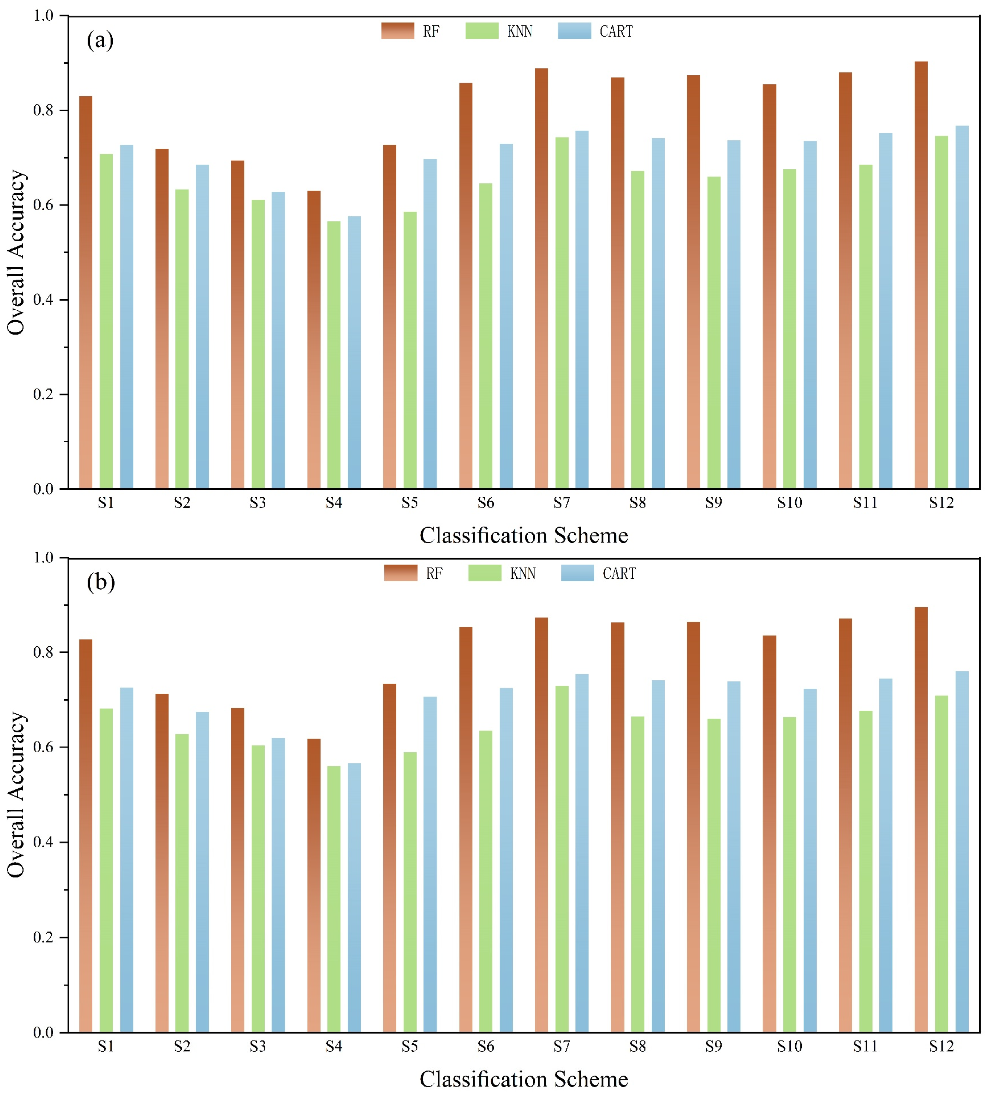
3.2. Classification Accuracy Assessment

The classification results depicted in Figure 4 indicate that RF consistently exhibits higher overall accuracy (OA) and Kappa coefficients than KNN and CART across all schemes in 2018 and 2022. In scheme S12, RF demonstrates an OA and Kappa coefficient of 90.33% and 0.82, respectively, for 2018, marking a 15.79% and 0.17 increase over KNN and CART. Similarly, in 2022, RF achieved an OA and Kappa coefficient of 89.59% and 0.81, respectively, surpassing KNN and CART by 16.71% and 0.18, respectively. Notably, RF-S12 exhibits the highest accuracy among all 12 schemes for both years. To compare the classification ability of each algorithm more intuitively, we analyzed their average highest accuracy results (Figure 5) and found that the descending order of OA and Kappa coefficients for each algorithm is RF > CART > KNN. Consequently, RF is identified as the best machine learning algorithm for forest-type recognition.

The comparison results of S1–S5, as illustrated in Figure 4, reveal that for single-feature forest type identification, the spectral feature (S1) consistently achieves the highest OA across RF, KNN, and CART for both years. In contrast, the geometric feature (S4) consistently yields the lowest OA. Consequently, S1 can be deemed the optimal single-feature scheme for forest-type identification. Conversely, when employing multi-feature combinations for forest type identification, S12 (WrapperSubsetEval preferred feature set) emerges with the highest OA across all algorithms in 2022 and all three algorithms in 2018. Although the KNN algorithm in 2022 exhibits slightly lower OA compared to S7 (spectral feature + vegetation index + texture feature + terrain feature) by 2%, the accuracy of the KNN algorithm across all schemes remains inferior to the other two algorithms. Thus, S12 can be regarded as the optimal feature combination scheme for forest-type identification.

Analyzing the changes in the accuracy of each algorithm, it can be found that different feature types have different impacts on the accuracy. By comparing S6–S10 and S11, respectively, it can be observed that in 2018, adding terrain features to S6 increased the OA by 2.23% to 3.88%; adding texture features to S8 increased the OA by 1.01% to 1.30%; adding vegetation indices to S9 increased the OA by 0.66% to 2.53%; adding spectral features to S10 increased the OA by 0.97% to 2.51%; and adding geometric features to S7 decreased the OA by 0.50% to 5.84%. In 2022, adding topographic features to S6 increased the OA by 1.77% to 4.16%; adding texture features to S8 increased the OA by 0.41% to 1.17%; adding vegetation indices to S9 increased the OA by 0.61% to 1.59%; adding spectral features to S10 increased the OA by 1.25% to 3.52%; and adding geometric features to S7 decreased the OA by 0.22% to 5.27%.

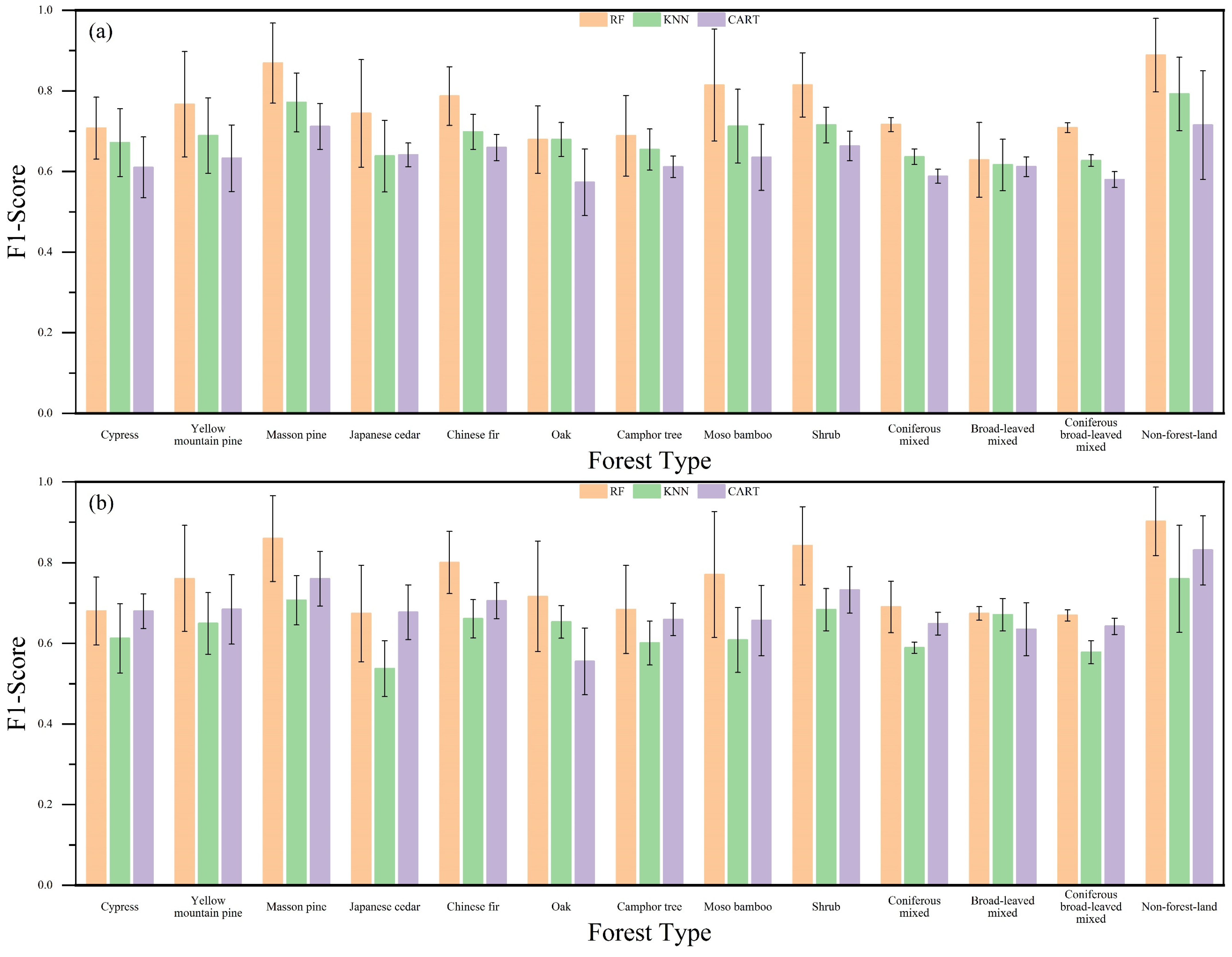
3.3. Tree Species Classification Results

From the F1-Score results for each forest type (Figure 6), Masson pine, shrub, and moso bamboo had higher F1-Scores than the other species, The F1-Scores for the three mixed forest species—coniferous mixed, broad-leaved mixed, and coniferous broad-leaved mixed—were relatively low and significantly lower than the results for other species. To further analyze the forest-type classification accuracy, we primarily compared the optimal feature combination schemes of each machine learning algorithm (Figure 7). Ultimately, six optimal combinations were identified: 2018-RF-S12, 2018-KNN-S12, 2018-CART-S12, 2022-RF-S12, 2022-KNN-S7, and 2022-CART-S12. The highest F1-Scores among the 2018 forest type were for Masson pine (RF-95.02%), shrub (RF-93.68%), and moso bamboo (RF-91.83%), with F1-Scores higher by 13.65% and 16.09%, 13.84% and 16.74%, and 17.81% and 18.50%, respectively, compared to the KNN and CART algorithms. In 2022, the highest F1-Scores among the forest type were for moso bamboo (RF-95.33%), Masson pine (RF-95.19%), and shrub (RF-89.50%), which were 16.97% and 17.31%, 12.59% and 16.12%, and 13.62% and 17.23% higher, respectively, compared to the KNN and CART algorithms. It can be seen that most forest types achieve optimal accuracy above 70%, indicating that all three machine learning algorithms can effectively distinguish subtropical forest types.

3.4. Feature Importance

The classification results revealed that the highest overall accuracy (OA) was achieved using the RF-S12 (the preferred feature subset) combination in both years. Consequently, we evaluated the importance of each feature in the RF model for forest-type identification globally and locally using the SHAP method based on the optimal accuracy scheme RF-S12 (Figure 8). The horizontal coordinate is the average absolute value of the SHAP values of all the features of the interpreted samples; the larger the value, the higher the importance of its corresponding feature, and the vertical coordinate represents the individual features, with each color representing the local feature importance of that feature for a forest type. By comparing the global importance of each feature, it was observed that altitude held the highest importance in 2018, followed by NDGI and Mean_B. Similarly, in 2022, altitude ranked the highest in importance, followed by Mean_B and NDGI. Figure 8 also illustrates the local importance of features in the identification of individual forest types, and it can be seen that altitude has the highest average SHAP value for distinguishing the majority of forest types. It can be seen that altitude has the highest SHAP value for most forest types, indicating that altitude plays an important role in the identification of subtropical forest types. However, altitude does not have the greatest contribution to the identification of every forest type. For example, in 2018, the most important influence on the identification of Japanese willow cedar was GNDVI, and in 2022, the most important influence on the identification of mosaic bamboo was the Angular Second Moment.

The combined results of evaluating the importance of variables in the two years indicate that Mean_B holds the highest importance among spectral features, NDGI ranks highest among the vegetation indices, Angular Second Moment is the most significant among texture features, and Main Direction holds the highest importance among geometric features. Additionally, altitude is identified as the most crucial variable among terrain features. Altitude, NDGI, and Mean_B consistently rank in the top three across both years, underscoring their pivotal role in forest type identification.

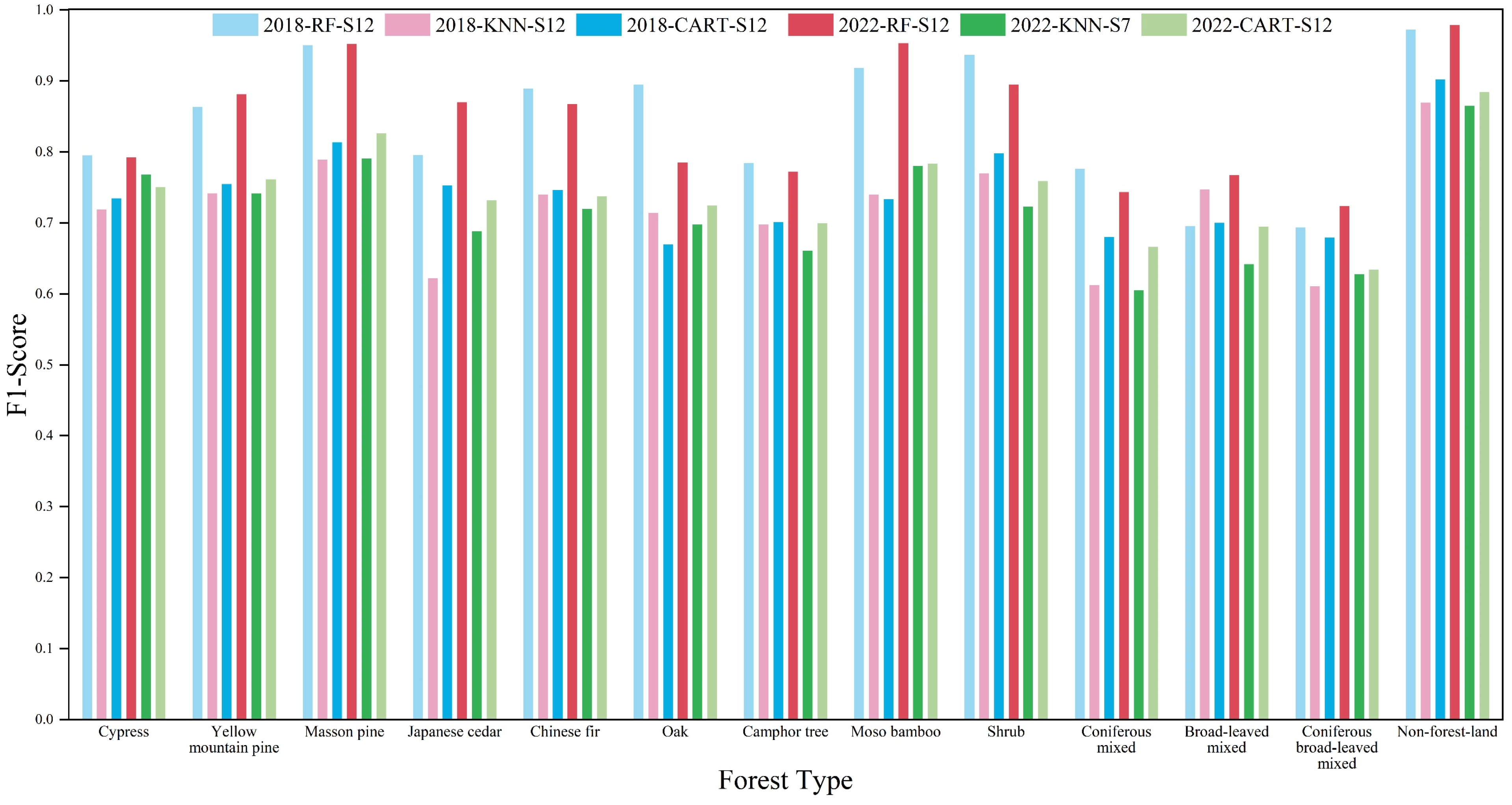
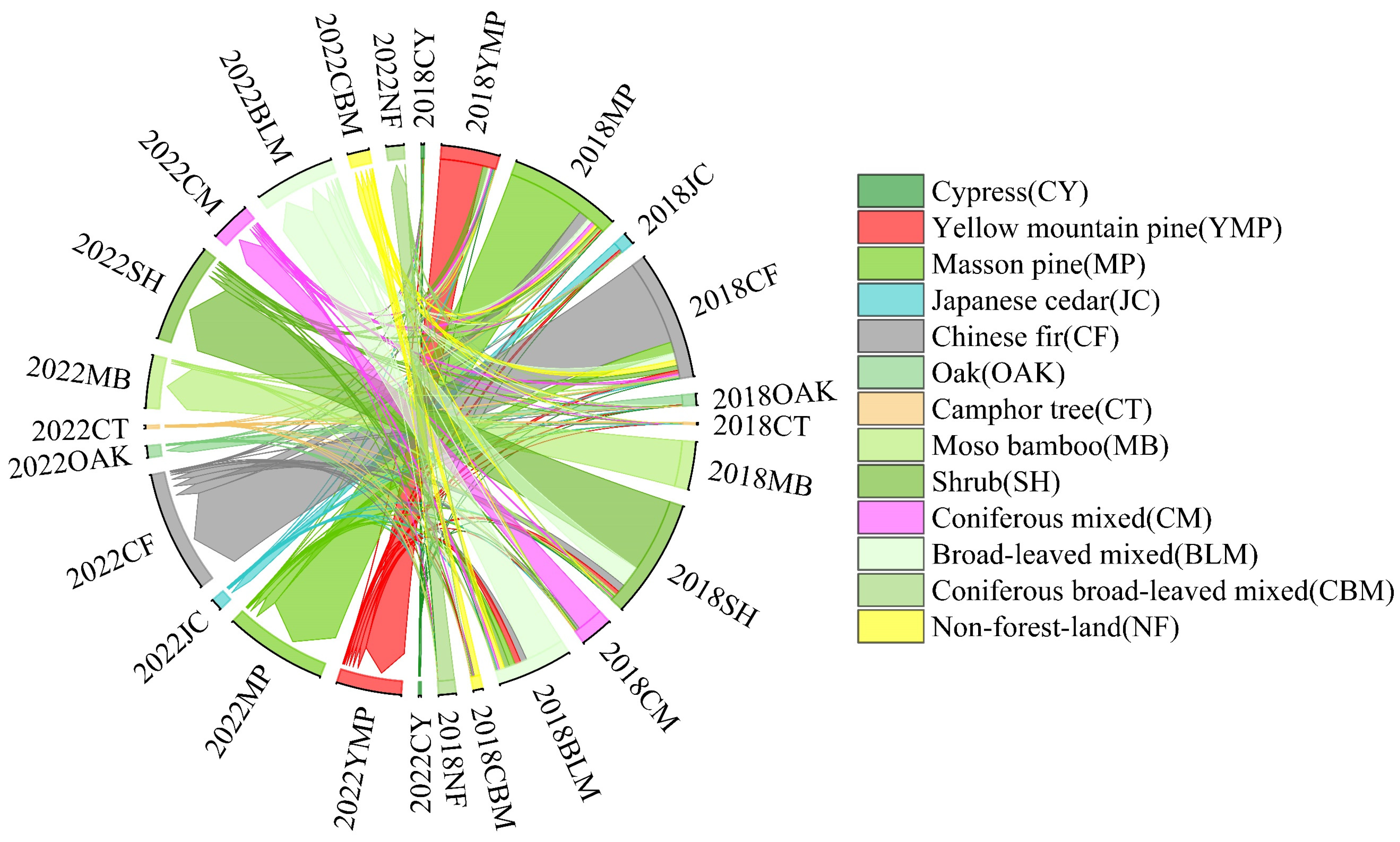
3.5. Changes in Forest Type from 2018 to 2022

Based on the optimal precision classification combinations for 2018-RF-S12 and 2022-RF-S12, classification result maps were generated (Figure 9). The areas of forest type were then extracted for transfer matrix analysis from 2018 to 2022 (Figure 10) to analyze the dynamics of dominant species in the study area. In 2018, the areas dominated by Chinese fir, shrub, and Masson pine accounted for the most significant shares, at 20.41%, 18.88%, and 17.87%, respectively. By 2022, the area shares of Chinese fir, Masson pine, and shrub decreased, with Chinese fir, Masson pine, and shrub remaining the most dominant species at 19.30%, 16.23%, and 15.78%, respectively. The increase in area from 2018 to 2022 included coniferous broad-leaved mixed, coniferous mixed, yellow mountain pine, broad-leaved mixed, moso bamboo, and camphor tree. Among these, coniferous broad-leaved mixed had the most significant increase, with an area increase of 417.53 hm², primarily due to Chinese fir being converted to coniferous broad-leaved mixed (204.18 hm²). Other notable increases included coniferous mixed by 255.37 hm², yellow mountain pine by 226.72 hm², broad-leaved mixed by 180.17 hm², moso bamboo by 175.23 hm², and camphor tree by 46.29 hm², with minimal increments in non-forested land and oak. From 2018 to 2022, there was a decrease in the area of shrub, Masson pine, and Chinese fir, with the largest reduction in shrub, which decreased by 686.19 hm². Most of this reduction was converted to broad-leaved mixed (776.44 hm²), followed by Masson pine and Chinese fir, decreasing by 360.85 hm² and 243.61 hm², respectively, primarily converted to coniferous mixed and yellow mountain pine. Japanese cedar and cypress also decreased, albeit by a smaller margin, at around 10 hm².

4. Discussion

4.1. Comparison of Machine Learning Algorithms

In this study, we conducted a comparative analysis of three machine learning algorithms—RF, KNN, and CART—to identify forest types in subtropical forests. The results show that the recognition accuracy of these algorithms is generally high, with the optimal OA exceeding 72%. Among them, RF exhibited the highest performance, outperforming KNN and CART. This finding is consistent with previous studies that highlight RF’s effectiveness in forest and land cover classification [56,57]. RF is advantageous as an integrated algorithm due to its excellent generalization capabilities and rapid operation speed, effectively addressing the limitations of single classifiers in performance enhancement. It exhibits high prediction accuracy, robustness to outliers and noise, and is less prone to overfitting. Additionally, RF can process high-dimensional and voluminous data in parallel, demonstrating greater stability and robustness against noise or isolated data points in the training set [58,59]. Due to these strengths, RF is widely utilized in the field of forest-type recognition [60]. Therefore, RF is more suitable among the three machine learning algorithms for identifying dominant forest type in subtropical forests using both GF-2 data and UAV multispectral data.

4.2. Comparison of Feature Combination Schemes

Among the three machine learning algorithms employed, the use of a multi-feature combination scheme resulted in higher accuracy compared to a single-feature scheme for classification. This is because tree species within the same forest type have similar features, making it difficult to distinguish them using only a single feature, especially in a subtropical forest area with high biodiversity and dense vegetation cover. Hurskainen et al. [61] used Formosat images and RF to classify the land use/land cover (LULC) category and found that the addition of auxiliary features improved OA by 6.1% to 16.5% compared to using a single feature. This indicates that combining multiple features can leverage the separability of different tree species across various features, thereby improving recognition accuracy [62].

Comparing the multi-feature combination schemes S6–S10 with S11 in 2018 and 2022 reveals that increasing topographic features, texture features, vegetation indices, and spectral features enhances accuracy. Notably, topographic features exhibit the most significant improvement in forest type recognition accuracy. Conversely, integrating geometric features leads to a decline in accuracy, suggesting a negative impact on classification accuracy. Guo et al. [63] also observed a negative effect of geometric features on OA, which decreased by 0.1% to 0.6% when geometric features were introduced. Although geometric features encompass attributes such as width, area, and length and provide useful information for forest type identification, they may also lead to feature redundancy, thus reducing accuracy [64,65]. The lower accuracy of S11, which incorporates all features, compared to S12, which comprises a subset of preferred features, may be attributed to the feature selection method employed in S12. This method selects essential features for classification while eliminating redundancy, enhancing model performance. Guo et al. [63] reached similar conclusions. Guo et al. found that using a subset of preferred features (30) yielded the highest classification accuracy, surpassing the accuracy obtained using all features (50).

4.3. Importance of Topographic Features in Classification

Upon analyzing the feature importance ranking, it becomes evident that altitude ranks highest within the optimal accuracy scheme for both years. Furthermore, all three terrain feature factors are consistently preferred in feature subset S12 across both years. This underscores the significant role of terrain features in identifying subtropical dominant forest type. Previous studies have reached similar conclusions. For example, Hościło et al. [66] utilized multi-temporal Sentinel-2 data to classify eight tree species and observed that topographic features played a pivotal role in tree species classification, leading to an increase in classification accuracy from 75.60% to 81.70% with the introduction of such features. Vorovencii et al. [67] utilized Sentinel-1 and Sentinel-2 time-series images to map tree species in low mountain areas. Their findings revealed a significant enhancement in classification accuracy upon incorporating topographic features, with elevation contributing most prominently, followed by slope direction and gradient. The reason for this is that the terrain type of the study area is a mid-mountain landform, and the vegetation types exhibit vertical distribution characteristics [68]. From the foot of the mountain to the top, the vegetation transitions from evergreen broadleaf forest, mixed evergreen and deciduous broadleaf forest, coniferous broad-leaved mixed forest, coniferous forest, to shrub. Additionally, the distribution of trees is closely related to topographic factors [69] due to the redistributive effects of altitude, slope, aspect, and other land features on surface light, heat, and water resources, which in turn affect the growth and distribution of tree species.

4.4. F1-Score Assessment and Dynamic Change Analysis

The F1-Score was computed to assess each machine learning algorithm’s capability in recognizing individual forest types. The F1-Score for broad-leaved mixed, coniferous mixed, and coniferous broad-leaved mixed forests was relatively lower than for other forest types. This discrepancy may stem from the complex characteristics of these mixed types, which encompass a variety of tree species and are prone to confusion during classification. Conversely, Masson pine, shrub, and moso bamboo exhibited higher F1-Scores. Their F1-Scores in the two-year optimal accuracy scheme ranked within the top three among tree species, likely due to their distinct leaf and crown shapes, which make them easily recognizable and less susceptible to confusion with other species.

Analyzing the area and changes in forest type in the study area from 2018 to 2022, it was found that Chinese fir, Masson pine, and shrub are the most widely distributed forest types, consistently ranking in the top three in terms of area proportions, while camphor tree and cypress have the smallest distribution areas. From 2018 to 2022, the area of coniferous broad-leaved mixed, coniferous mixed, yellow mountain pine, broad-leaved mixed, and moso bamboo increased, whereas the area of shrub, Masson pine, and Chinese fir decreased. The increase in mixed tree species is related to continuous artificial afforestation, stand renovation, and forest closure measures aimed at enriching stand structure and increasing biodiversity [68]. The increase in yellow mountain pine is likely due to its strong adaptability to the climate, terrain, and soil of the study area, giving it a competitive advantage. Masson pine and Chinese fir, which overlap significantly with yellow mountain pine in ecological niches, are disadvantaged in resource competition. The increase in moso bamboo is primarily due to its fast growth characteristics. Shrubs, concentrated in the high-altitude areas of the study region, are less affected by human activities and gradually grow into secondary restorative trees with time and the implementation of ecosystem protection policies.

4.5. Limitations and Future Research Perspectives

The segmentation scale significantly influences the accuracy of object-oriented classification [70]. We used ESP2 to determine the optimal segmentation scale, and this approach not only reduces the subjectivity in scale selection but also improves the efficiency of image segmentation. However, it provides only a limited selection, requiring visual discrimination to finalize the optimal scale, which is not fully objective or automated. Future research should focus on methods to automatically determine segmentation parameters to improve segmentation accuracy and automation. Meanwhile, quantitative indicators are used to evaluate the segmentation performance more comprehensively. This study primarily evaluates traditional machine learning algorithms. Deep learning models, a deep artificial neural network approach that has garnered significant attention in recent years [71], can notably enhance the classification accuracy of land cover types compared to traditional machine learning methods, particularly in regions with complex land cover types [72,73]. Future research should compare these deep learning methods to potentially improve the mapping accuracy of forest types. Feature selection is a critical step in the classification process. It can improve the computational performance of the classifier by removing redundant information and addressing the time-consuming issue of processing all available features [74]. In this study, we used only one feature optimization method (WrapperSubsetEval), but no single method is optimal across different machine learning algorithms, climatic conditions, and remote sensing data types. Therefore, future research needs to explore various feature selection methods tailored to specific objectives. While most forest types achieved high accuracy, the F1-Scores of three mixed forest species groups—broadleaf mixed, coniferous mixed, and coniferous broad mixed—were relatively low. We intend to incorporate multi-source remote sensing data, such as integrating three-dimensional remote sensing data like LiDAR, to extract richer distinguishing features from spatial structural information in our subsequent studies. This effort aims to further develop and optimize classification algorithms, considering the integration of advanced deep learning methods to better accommodate the complexity of mixed forests and thereby enhance the accuracy and applicability of classification results. Due to data constraints, this study utilized only two GF-2 images over a four-year period for forest-type identification analysis. Long-term forest vegetation dynamics require extended analytical periods. With the increasing resolution of satellite data, regular annual monitoring of forest vegetation in subtropical regions is crucial for tracking temporal changes. In the future, we plan to expand data collection to encompass more time points, thereby capturing the dynamic changes in forest biodiversity more effectively.

5. Conclusions

This study leveraged GF-2 satellite and UAV multispectral images to assess the efficacy of different feature combination schemes and machine learning algorithms in identifying subtropical forest types using an object-oriented approach. Our results indicate that the Random Forest (RF) algorithm, particularly with the optimized feature combination Scheme S12 (S12), outperformed others, demonstrating the highest classification accuracy. Multi-feature schemes proved more effective than single-feature schemes, with topographic features significantly enhancing accuracy, whereas geometric features reduced it. Our analysis of feature importance highlighted the critical roles of altitude, NDGI, and Mean_B in forest type identification, with Masson pine, shrub, and moso bamboo achieving notably high F1-Scores. Over the study period, we observed a transition in forest type from single-story structures to mixed forest structures, enhancing ecological diversity and stability. Using the RF algorithm and Scheme S12, we successfully identified forest types in the Lushan National Nature Reserve for 2018 and 2022, achieving optimal classification accuracy. This study underscores the potential of GF-2 images for large-scale, refined forest-type identification and monitoring in subtropical forests, offering insights that enhance forest management and biodiversity conservation efforts.

References

1. Romijn, E.; Lantican, C.B.; Herold, M.; Lindquist, E.; Ochieng, R.; Wijaya, A.; Murdiyarso, D.; Verchot, L. Assessing Change in National Forest Monitoring Capacities of 99 Tropical Countries. For. Ecol. Manag. 2015, 352, 109–123. [Google Scholar] [CrossRef]
2. Torabzadeh, H.; Leiterer, R.; Hueni, A.; Schaepman, M.E.; Morsdorf, F. Tree Species Classification in a Temperate Mixed Forest Using a Combination of Imaging Spectroscopy and Airborne Laser Scanning. Agric. For. Meteorol. 2019, 279, 107744. [Google Scholar] [CrossRef]
3. Crabbe, R.A.; Lamb, D.; Edwards, C. Discrimination of Species Composition Types of a Grazed Pasture Landscape Using Sentinel-1 and Sentinel-2 Data. Int. J. Appl. Earth Obs. Geoinf. 2020, 84, 101978. [Google Scholar] [CrossRef]
4. Lei, Z.; Li, H.; Zhao, J.; Jing, L.; Tang, Y.; Wang, H. Individual Tree Species Classification Based on a Hierarchical Convolutional Neural Network and Multitemporal Google Earth Images. Remote Sens. 2022, 14, 5124. [Google Scholar] [CrossRef]
5. Wang, M.; Zheng, Y.; Huang, C.; Meng, R.; Pang, Y.; Jia, W.; Zhou, J.; Huang, Z.; Fang, L.; Zhao, F. Assessing Landsat-8 and Sentinel-2 Spectral-Temporal Features for Mapping Tree Species of Northern Plantation Forests in Heilongjiang Province, China. For. Ecosyst. 2022, 9, 100032. [Google Scholar] [CrossRef]
6. Shi, Y.; Wang, T.; Skidmore, A.K.; Heurich, M. Improving LiDAR-Based Tree Species Mapping in Central European Mixed Forests Using Multi-Temporal Digital Aerial Colour-Infrared Photographs. Int. J. Appl. Earth Obs. Geoinf. 2020, 84, 101970. [Google Scholar] [CrossRef]
7. Cilek, A.; Berberoglu, S.; Donmez, C.; Sahingoz, M. The Use of Regression Tree Method for Sentinel-2 Satellite Data to Mapping Percent Tree Cover in Different Forest Types. Environ. Sci. Pollut. Res. 2022, 29, 23665–23676. [Google Scholar] [CrossRef]
8. Becker, A.; Russo, S.; Puliti, S.; Lang, N.; Schindler, K.; Wegner, J.D. Country-Wide Retrieval of Forest Structure from Optical and SAR Satellite Imagery with Deep Ensembles. ISPRS J. Photogramm. Remote Sens. 2023, 195, 269–286. [Google Scholar] [CrossRef]
9. Ganivet, E.; Bloomberg, M. Towards Rapid Assessments of Tree Species Diversity and Structure in Fragmented Tropical Forests: A Review of Perspectives Offered by Remotely-Sensed and Field-Based Data. Forest Ecol. Manag. 2019, 432, 40–53. [Google Scholar] [CrossRef]
10. Wang, R.; Gamon, J.A. Remote Sensing of Terrestrial Plant Biodiversity. Remote Sens. Environ. 2019, 231, 111218. [Google Scholar] [CrossRef]
11. Reddy, C.S.; Kurian, A.; Srivastava, G.; Singhal, J.; Varghese, A.O.; Padalia, H.; Ayyappan, N.; Rajashekar, G.; Jha, C.S.; Rao, P.V.N. Remote Sensing Enabled Essential Biodiversity Variables for Biodiversity Assessment and Monitoring: Technological Advancement and Potentials. Biodivers. Conserv. 2021, 30, 1–14. [Google Scholar] [CrossRef]
12. Axelsson, A.; Lindberg, E.; Reese, H.; Olsson, H. Tree Species Classification Using Sentinel-2 Imagery and Bayesian Inference. Int. J. Appl. Earth Obs. Geoinf. 2021, 100, 102318. [Google Scholar] [CrossRef]
13. Bolyn, C.; Lejeune, P.; Michez, A.; Latte, N. Mapping Tree Species Proportions from Satellite Imagery Using Spectral-Spatial Deep Learning. Remote Sens. Environ. 2022, 280, 113205. [Google Scholar] [CrossRef]
14. Mäyrä, J.; Keski-Saari, S.; Kivinen, S.; Tanhuanpää, T.; Hurskainen, P.; Kullberg, P.; Poikolainen, L.; Viinikka, A.; Tuominen, S.; Kumpula, T.; et al. Tree Species Classification from Airborne Hyperspectral and LiDAR Data Using 3D Convolutional Neural Networks. Remote Sens. Environ. 2021, 256, 112322. [Google Scholar] [CrossRef]
15. Matese, A.; Toscano, P.; Di Gennaro, S.F.; Genesio, L.; Vaccari, F.P.; Primicerio, J.; Belli, C.; Zaldei, A.; Bianconi, R.; Gioli, B. Intercomparison of UAV, Aircraft and Satellite Remote Sensing Platforms for Precision Viticulture. Remote Sens. 2015, 7, 2971–2990. [Google Scholar] [CrossRef]
16. Sprott, A.H.; Piwowar, J.M. How to Recognize Different Types of Trees from Quite a Long Way Away: Combining UAV and Spaceborne Imagery for Stand-Level Tree Species Identification. J. Unmanned Veh. Syst. 2021, 9, 166–181. [Google Scholar] [CrossRef]
17. Chen, X.; Shen, X.; Cao, L. Tree Species Classification in Subtropical Natural Forests Using High-Resolution UAV RGB and SuperView-1 Multispectral Imageries Based on Deep Learning Network Approaches: A Case Study within the Baima Snow Mountain National Nature Reserve, China. Remote Sens. 2023, 15, 2697. [Google Scholar] [CrossRef]
18. Hidayat, S.; Matsuoka, M.; Baja, S.; Rampisela, D.A. Object-Based Image Analysis for Sago Palm Classification: The Most Important Features from High-Resolution Satellite Imagery. Remote Sens. 2018, 10, 1319. [Google Scholar] [CrossRef]
19. Rajbhandari, S.; Aryal, J.; Osborn, J.; Lucieer, A.; Musk, R. Leveraging Machine Learning to Extend Ontology-Driven Geographic Object-Based Image Analysis (O-GEOBIA): A Case Study in Forest-Type Mapping. Remote Sens. 2019, 11, 503. [Google Scholar] [CrossRef]
20. Feizizadeh, B.; Kazemi Garajeh, M.; Blaschke, T.; Lakes, T. An Object Based Image Analysis Applied for Volcanic and Glacial Landforms Mapping in Sahand Mountain, Iran. Catena 2021, 198, 105073. [Google Scholar] [CrossRef]
21. Qu, L.; Chen, Z.; Li, M.; Zhi, J.; Wang, H. Accuracy Improvements to Pixel-Based and Object-Based LULC Classification with Auxiliary Datasets from Google Earth Engine. Remote Sens. 2021, 13, 453. [Google Scholar] [CrossRef]
22. Deur, M.; Gasparovic, M.; Balenovic, I. An Evaluation of Pixel- and Object-Based Tree Species Classification in Mixed Deciduous Forests Using Pansharpened Very High Spatial Resolution Satellite Imagery. Remote Sens. 2021, 13, 1868. [Google Scholar] [CrossRef]
23. Li, T.; Johansen, K.; McCabe, M.F. A Machine Learning Approach for Identifying and Delineating Agricultural Fields and Their Multi-Temporal Dynamics Using Three Decades of Landsat Data. ISPRS J. Photogramm. Remote Sens. 2022, 186, 83–101. [Google Scholar] [CrossRef]
24. Zeferino, L.B.; Tavares de Souza, L.F.; do Amaral, C.H.; Fernandes Filho, E.I.; de Oliveira, T.S. Does Environmental Data Increase the Accuracy of Land Use and Land Cover Classification? Int. J. Appl. Earth Obs. Geoinf. 2020, 91, 102128. [Google Scholar] [CrossRef]
25. Oreti, L.; Giuliarelli, D.; Tomao, A.; Barbati, A. Object Oriented Classification for Mapping Mixed and Pure Forest Stands Using Very-High Resolution Imagery. Remote Sens. 2021, 13, 2508. [Google Scholar] [CrossRef]
26. Wang, M.; Liu, Z.; Baig, M.H.A.; Wang, Y.; Li, Y.; Chen, Y. Mapping Sugarcane in Complex Landscapes by Integrating Multi-Temporal Sentinel-2 Images and Machine Learning Algorithms. Land Use Policy 2019, 88, 104190. [Google Scholar] [CrossRef]
27. Fang, J.; Guo, Z.; Hu, H.; Kato, T.; Muraoka, H.; Son, Y. Forest Biomass Carbon Sinks in East Asia, with Special Reference to the Relative Contributions of Forest Expansion and Forest Growth. Glob. Change Biol. 2014, 20, 2019–2030. [Google Scholar] [CrossRef]
28. Xiang, X.-G.; Mi, X.-C.; Zhou, H.-L.; Jianwu, L.; Chung, S.-W.; Li, D.-Z.; Huang, W.-C.; Jin, W.-T.; Li, Z.-Y.; Huang, L.-Q.; et al. Biogeographical Diversification of Mainland Asian Dendrobium (Orchidaceae) and Its Implications for the Historical Dynamics of Evergreen Broad-Leaved Forests. J. Biogeogr. 2016, 43, 1310–1323. [Google Scholar] [CrossRef]
29. Xu, Z.; Shen, X.; Cao, L.; Coops, N.C.; Goodbody, T.R.H.; Zhong, T.; Zhao, W.; Sun, Q.; Ba, S.; Zhang, Z.; et al. Tree Species Classification Using UAS-Based Digital Aerial Photogrammetry Point Clouds and Multispectral Imageries in Subtropical Natural Forests. Int. J. Appl. Earth Obs. Geoinf. 2020, 92, 102173. [Google Scholar] [CrossRef]
30. Richter, R.; Reu, B.; Wirth, C.; Doktor, D.; Vohland, M. The Use of Airborne Hyperspectral Data for Tree Species Classification in a Species-Rich Central European Forest Area. Int. J. Appl. Earth Obs. Geoinf. 2016, 52, 464–474. [Google Scholar] [CrossRef]
31. Fassnacht, F.E.; Latifi, H.; Stereńczak, K.; Modzelewska, A.; Lefsky, M.; Waser, L.T.; Straub, C.; Ghosh, A. Review of Studies on Tree Species Classification from Remotely Sensed Data. Remote Sens. Environ. 2016, 186, 64–87. [Google Scholar] [CrossRef]
32. Liu, Y.; Zhang, R.; Lin, C.-F.; Zhang, Z.; Zhang, R.; Shang, K.; Zhao, M.; Huang, J.; Wang, X.; Li, Y.; et al. Remote Sensing of Subtropical Tree Diversity: The Underappreciated Roles of the Practical Definition of Forest Canopy and Phenological Variation. For. Ecosyst. 2023, 10, 100122. [Google Scholar] [CrossRef]
33. Sothe, C.; Dalponte, M.; de Almeida, C.M.; Schimalski, M.B.; Lima, C.L.; Liesenberg, V.; Miyoshi, G.T.; Garcia Tommaselli, A.M. Tree Species Classification in a Highly Diverse Subtropical Forest Integrating UAV-Based Photogrammetric Point Cloud and Hyperspectral Data. Remote Sens. 2019, 11, 1338. [Google Scholar] [CrossRef]
34. Qin, H.; Zhou, W.; Yao, Y.; Wang, W. Individual Tree Segmentation and Tree Species Classification in Subtropical Broadleaf Forests Using UAV-Based LiDAR, Hyperspectral, and Ultrahigh-Resolution RGB Data. Remote Sens. Environ. 2022, 280, 113143. [Google Scholar] [CrossRef]
35. Wu, Q.; Zhong, R.; Zhao, W.; Song, K.; Du, L. Land-Cover Classification Using GF-2 Images and Airborne Lidar Data Based on Random Forest. Int. J. Remote Sens. 2019, 40, 2410–2426. [Google Scholar] [CrossRef]
36. Li, D.; Ke, Y.; Gong, H.; Li, X. Object-Based Urban Tree Species Classification Using Bi-Temporal WorldView-2 and WorldView-3 Images. Remote Sens. 2015, 7, 16917–16937. [Google Scholar] [CrossRef]
37. Jia, K.; Liu, J.; Tu, Y.; Li, Q.; Sun, Z.; Wei, X.; Yao, Y.; Zhang, X. Land Use and Land Cover Classification Using Chinese GF-2 Multispectral Data in a Region of the North China Plain. Front Earth Sci. 2019, 13, 327–335. [Google Scholar] [CrossRef]
38. Drǎguţ, L.; Tiede, D.; Levick, S.R. ESP: A Tool to Estimate Scale Parameter for Multiresolution Image Segmentation of Remotely Sensed Data. Int. J. Geogr. Inf. Sci. 2010, 24, 859–871. [Google Scholar] [CrossRef]
39. Woodcock, C.E.; Strahler, A.H. The Factor of Scale in Remote Sensing. Remote Sens. Environ. 1987, 21, 311–332. [Google Scholar] [CrossRef]
40. Ferreira, M.P.; Zortea, M.; Zanotta, D.C.; Shimabukuro, Y.E.; de Souza Filho, C.R. Mapping Tree Species in Tropical Seasonal Semi-Deciduous Forests with Hyperspectral and Multispectral Data. Remote Sens. Environ. 2016, 179, 66–78. [Google Scholar] [CrossRef]
41. Clark, M.L.; Kilham, N.E. Mapping of Land Cover in Northern California with Simulated Hyperspectral Satellite Imagery. ISPRS J. Photogramm. Remote Sens. 2016, 119, 228–245. [Google Scholar] [CrossRef]
42. Wood, E.M.; Pidgeon, A.M.; Radeloff, V.C.; Keuler, N.S. Image Texture as a Remotely Sensed Measure of Vegetation Structure. Remote Sens. Environ. 2012, 121, 516–526. [Google Scholar] [CrossRef]
43. Olofsson, P.; Foody, G.M.; Herold, M.; Stehman, S.V.; Woodcock, C.E.; Wulder, M.A. Good Practices for Estimating Area and Assessing Accuracy of Land Change. Remote Sens. Environ. 2014, 148, 42–57. [Google Scholar] [CrossRef]
44. Dong, C.; Zhao, G.; Meng, Y.; Li, B.; Peng, B. The Effect of Topographic Correction on Forest Tree Species Classification Accuracy. Remote Sens. 2020, 12, 787. [Google Scholar] [CrossRef]
45. Zhao, Q.; Jia, S.; Li, Y. Hyperspectral Remote Sensing Image Classification Based on Tighter Random Projection with Minimal Intra-Class Variance Algorithm. Pattern Recognit. 2021, 111, 107635. [Google Scholar] [CrossRef]
46. Qin, H.; Wang, W.; Yao, Y.; Qian, Y.; Xiong, X.; Zhou, W. First Experience with Zhuhai-1 Hyperspectral Data for Urban Dominant Tree Species Classification in Shenzhen, China. Remote Sens. 2023, 15, 3179. [Google Scholar] [CrossRef]
47. Pal, M. Random Forest Classifier for Remote Sensing Classification. Int. J. Remote Sens. 2005, 26, 217–222. [Google Scholar] [CrossRef]
48. Haapanen, R.; Ek, A.R.; Bauer, M.E.; Finley, A.O. Delineation of Forest/Nonforest Land Use Classes Using Nearest Neighbor Methods. Remote Sens. Environ. 2004, 89, 265–271. [Google Scholar] [CrossRef]
49. Tu, Y.; Lang, W.; Yu, L.; Li, Y.; Jiang, J.; Qin, Y.; Wu, J.; Chen, T.; Xu, B. Improved Mapping Results of 10 m Resolution Land Cover Classification in Guangdong, China Using Multisource Remote Sensing Data with Google Earth Engine. IEEE J. Sel. Topics Appl. Earth Observ. Remote Sens. 2020, 13, 5384–5397. [Google Scholar] [CrossRef]
50. Luo, C.; Qi, B.; Liu, H.; Guo, D.; Lu, L.; Fu, Q.; Shao, Y. Using Time Series Sentinel-1 Images for Object-Oriented Crop Classification in Google Earth Engine. Remote Sens. 2021, 13, 561. [Google Scholar] [CrossRef]
51. Chen, C.; Jing, L.; Li, H.; Tang, Y.; Chen, F. Individual Tree Species Identification Based on a Combination of Deep Learning and Traditional Features. Remote Sens. 2023, 15, 2301. [Google Scholar] [CrossRef]
52. Baumann, M.; Ozdogan, M.; Kuemmerle, T.; Wendland, K.J.; Esipova, E.; Radeloff, V.C. Using the Landsat Record to Detect Forest-Cover Changes during and after the Collapse of the Soviet Union in the Temperate Zone of European Russia. Remote Sens. Environ. 2012, 124, 174–184. [Google Scholar] [CrossRef]
53. Lundberg, S.M.; Lee, S.-I. A Unified Approach to Interpreting Model Predictions. In Advances in Neural Information Processing Systems 30, Proceedings of the 31st International Conference on Neural Information Processing Systems, Long Beach, CA, USA, 4–9 December 2017; Guyon, I., Von Luxburg, U., Bengio, S., Wallach, H., Fergus, R., Vishwanathan, S., Garnett, R., Eds.; Curran Associates Inc.: Red Hook, NY, USA, 2017; pp. 4768–4777. [Google Scholar]
54. Shapley, L.S. A Value for N-Person Games; RAND Corporation: Santa Monica, CA, USA, 1952. [Google Scholar]
55. Dikshit, A.; Pradhan, B. Interpretable and Explainable AI (XAI) Model for Spatial Drought Prediction. Sci. Total Environ. 2021, 801, 149797. [Google Scholar] [CrossRef]
56. Rina, S.; Ying, H.; Shan, Y.; Du, W.; Liu, Y.; Li, R.; Deng, D. Application of Machine Learning to Tree Species Classification Using Active and Passive Remote Sensing: A Case Study of the Duraer Forestry Zone. Remote Sens. 2023, 15, 2596. [Google Scholar] [CrossRef]
57. Luo, H.; Li, M.; Dai, S.; Li, H.; Li, Y.; Hu, Y.; Zheng, Q.; Yu, X.; Fang, J. Combinations of Feature Selection and Machine Learning Algorithms for Object-Oriented Betel Palms and Mango Plantations Classification Based on Gaofen-2 Imagery. Remote Sens. 2022, 14, 1757. [Google Scholar] [CrossRef]
58. Melville, B.; Lucieer, A.; Aryal, J. Object-Based Random Forest Classification of Landsat ETM plus and WorldView-2 Satellite Imagery for Mapping Lowland Native Grassland Communities in Tasmania, Australia. Int. J. Appl. Earth Obs. Geoinf. 2018, 66, 46–55. [Google Scholar] [CrossRef]
59. Wurm, M.; Taubenböck, H.; Weigand, M.; Schmitt, A. Slum Mapping in Polarimetric SAR Data Using Spatial Features. Remote Sens. Environ. 2017, 194, 190–204. [Google Scholar] [CrossRef]
60. Liu, L.; Coops, N.C.; Aven, N.W.; Pang, Y. Mapping Urban Tree Species Using Integrated Airborne Hyperspectral and LiDAR Remote Sensing Data. Remote Sens. Environ. 2017, 200, 170–182. [Google Scholar] [CrossRef]
61. Hurskainen, P.; Adhikari, H.; Siljander, M.; Pellikka, P.K.E.; Hemp, A. Auxiliary Datasets Improve Accuracy of Object-Based Land Use/Land Cover Classification in Heterogeneous Savanna Landscapes. Remote Sens. Environ. 2019, 233, 111354. [Google Scholar] [CrossRef]
62. Hua, L.; Zhang, X.; Chen, X.; Yin, K.; Tang, L. A Feature-Based Approach of Decision Tree Classification to Map Time Series Urban Land Use and Land Cover with Landsat 5 TM and Landsat 8 OLI in a Coastal City, China. ISPRS Int. J. Geoinf. 2017, 6, 331. [Google Scholar] [CrossRef]
63. Guo, Q.; Zhang, J.; Guo, S.; Ye, Z.; Deng, H.; Hou, X.; Zhang, H. Urban Tree Classification Based on Object-Oriented Approach and Random Forest Algorithm Using Unmanned Aerial Vehicle (UAV) Multispectral Imagery. Remote Sens. 2022, 14, 3885. [Google Scholar] [CrossRef]
64. Fu, B.; Liu, M.; He, H.; Lan, F.; He, X.; Liu, L.; Huang, L.; Fan, D.; Zhao, M.; Jia, Z. Comparison of Optimized Object-Based RF-DT Algorithm and SegNet Algorithm for Classifying Karst Wetland Vegetation Communities Using Ultra-High Spatial Resolution UAV Data. Int. J. Appl. Earth Obs. Geoinf. 2021, 104, 102553. [Google Scholar] [CrossRef]
65. Garg, R.; Kumar, A.; Prateek, M.; Pandey, K.; Kumar, S. Land Cover Classification of Spaceborne Multifrequency SAR and Optical Multispectral Data Using Machine Learning. Adv. Space Res. 2022, 69, 1726–1742. [Google Scholar] [CrossRef]
66. Hościło, A.; Lewandowska, A. Mapping Forest Type and Tree Species on a Regional Scale Using Multi-Temporal Sentinel-2 Data. Remote Sens. 2019, 11, 929. [Google Scholar] [CrossRef]
67. Vorovencii, I.; Dincă, L.; Crișan, V.; Postolache, R.-G.; Codrean, C.-L.; Cătălin, C.; Greșiță, C.I.; Chima, S.; Gavrilescu, I. Local-Scale Mapping of Tree Species in a Lower Mountain Area Using Sentinel-1 and -2 Multitemporal Images, Vegetation Indices, and Topographic Information. Front. For. Glob. Change 2023, 6, 1220253. [Google Scholar] [CrossRef]
68. He, G.; Zhang, Z.; Zhu, Q.; Wang, W.; Peng, W.; Cai, Y. Estimating Carbon Sequestration Potential of Forest and Its Influencing Factors at Fine Spatial-Scales: A Case Study of Lushan City in Southern China. Int. J. Environ. Res. Public Health 2022, 19, 9184. [Google Scholar] [CrossRef]
69. Oke, O.A.; Thompson, K.A. Distribution Models for Mountain Plant Species: The Value of Elevation. Ecol. Model. 2015, 301, 72–77. [Google Scholar] [CrossRef]
70. Zhao, F.; Wu, X.; Wang, S. Object-Oriented Vegetation Classification Method Based on UAV and Satellite Image Fusion. Procedia Comput. Sci. 2020, 174, 609–615. [Google Scholar] [CrossRef]
71. Reichstein, M.; Camps-Valls, G.; Stevens, B.; Jung, M.; Denzler, J.; Carvalhais, N.; Prabhat, F. Deep Learning and Process Understanding for Data-Driven Earth System Science. Nature 2019, 566, 195–204. [Google Scholar] [CrossRef]
72. Zhang, C.; Pan, X.; Li, H.; Gardiner, A.; Sargent, I.; Hare, J.; Atkinson, P.M. A Hybrid MLP-CNN Classifier for Very Fine Resolution Remotely Sensed Image Classification. ISPRS J. Photogramm. Remote Sens. 2018, 140, 133–144. [Google Scholar] [CrossRef]
73. Onishi, M.; Watanabe, S.; Nakashima, T.; Ise, T. Practicality and Robustness of Tree Species Identification Using UAV RGB Image and Deep Learning in Temperate Forest in Japan. Remote Sens. 2022, 14, 1710. [Google Scholar] [CrossRef]
74. Zhou, R.; Yang, C.; Li, E.; Cai, X.; Yang, J.; Xia, Y. Object-Based Wetland Vegetation Classification Using Multi-Feature Selection of Unoccupied Aerial Vehicle RGB Imagery. Remote Sens. 2021, 13, 4910. [Google Scholar] [CrossRef]
Figure 1. Location of study area. (a,b) Jiangxi Province, China; (c) Spatial distribution of field survey plots, and UAV monitoring sites.
Forests 15 01327 g001
Figure 2. (a) 2018 GF-2 image; (b) 2022 GF-2 image; (c,d) 2023 UAV multispectral images.
Forests 15 01327 g002
Figure 3. The estimation of the scales using the ESP2 tool. (a) 2018; (b) 2022.
Forests 15 01327 g003
Figure 4. Overall accuracy of classification schemes. (a) 2018; (b) 2022.
Forests 15 01327 g004
Figure 5. Accuracy comparison of algorithms. (a) 2018; (b) 2022.
Forests 15 01327 g005
Figure 6. Comparison of F1-Scores of different forest types. (a) 2018; (b) 2022.
Forests 15 01327 g006
Figure 7. F1-Scores of different schemes for different forest types.
Forests 15 01327 g007
Figure 8. Feature importance ranking results. (a) 2018; (b) 2022.
Forests 15 01327 g008
Figure 9. Classification results of the optimal accuracy classification combination in 2018 and 2022 (a) 2018; (b) 2022.
Forests 15 01327 g009
Figure 10. Dynamic changes in forest type from 2018 to 2022.
Forests 15 01327 g010